REPRESENTATION OF UNCERTAINTY AND CORRIDOR DP FOR HYDROPOWER OPTIMIZATION
A Dissertation
Presented to the Faculty of the Graduate School of Cornell University
In Partial Fulfillment of the Requirements for the Degree of Doctor of Philosophy
by
Jonathan Richard Lamontagne
REPRESENTATION OF UNCERTAINTY AND CORRIDOR DP FOR HYDROPOWER OPTIMIZATION
Jonathan Richard Lamontagne, Ph.D. Cornell University 2015
This thesis focuses on optimization techniques for multi-reservoir hydropower systems operation, with a particular concern with the representation and impact of uncertainty. The thesis reports on three research investigations: 1) examination of the impact of uncertainty representations, 2) efficient solution methods for multi-reservoir stochastic dynamic programming (SDP) models, and 3) diagnostic analyses for
hydropower system operation.
The first investigation explores the value of sophistication in the representation of forecast and inflow uncertainty in stochastic hydropower optimization models using a sampling SDP (SSDP) model framework. SSDP models with different uncertainty representation ranging in sophistication from simple deterministic to complex dynamic stochastic models are employed when optimize a single reservoir systems [similar to Faber and Stedinger, 2001]. The effect of uncertainty representation on simulated system performance is examined with varying storage and powerhouse capacity, and with random or mean energy prices. In many cases very simple uncertainty models perform as well as more complex ones, but not always.
The second investigation develops a new and efficient algorithm for solving multi-reservoir SDP models: Corridor SDP. Rather than employing a uniform grid across the entire state space, Corridor SDP efficiently concentrates points in where the
system is likely to visit, as determined by historical operations or simulation. Radial basis functions (RBFs) are used for interpolation. A greedy algorithm places points where they are needed to achieve a good approximation. In a four-reservoir test case, Corridor DP achieves the same accuracy as spline-DP and linear-DP with
approximately 1/10 and 1/1100 the number of discrete points, respectively. When local curvature is more pronounced (due to minimum-flow constraints), Corridor DP achieves the same accuracy as spline-DP and linear-DP with approximately 1/30 and 1/215 the number of points, respectively.
The third investigation explores three diagnostic approaches for analyzing hydropower system operation. First, several simple diagnostic statistics describe reservoir volume and powerhouse capacity in units of time, allowing scale-invariant comparisons and classification of different reservoir systems and their operation. Second, a regression analysis using optimal storage/release sequences identifies the most useful hydrologic state variables . Finally spectral density estimation identifies critical time scales for operation for several single-reservoir systems considering mean and random energy prices.
Deregulation of energy markets has made optimization of hydropower operations an active concern. Another development is publication of Extended Streamflow Forecasts (ESP) by the National Weather Service (NWS) and others to describe flow forecasts and their precision; the multivariate Sampling SDP models employed here are appropriately structured to incorporate such information in
operational hydropower decisions. This research contributes to our ability to structure and build effective hydropower optimization models.
BIOGRAPHICAL SKETCH
Jonathan Richard Lamontagne was born in Nashua, New Hampshire on November 11, 1986. After obtaining his high school diploma at Pembroke Academy in Pembroke, New Hampshire he attended the University of New Hampshire where he received a B.S. in Civil Engineering in 2009. During summer and winter breaks he worked as a construction laborer, an engineering intern for Appledore Engineering, and as a hazardous waste enforcement intern for the New Hampshire Department of Environmental Services. He entered graduate studies at Cornell in 2009 to pursue a lifelong interest in water resources engineering, and received his M.S. in Civil and Environmental Engineering in 2014. Upon graduation he accepted a post-doctoral research position at Cornell. He currently lives in Ithaca with his wife Katie.
This thesis is dedicated to the generations of my family who made my success possible, and especially to my Katie.
ACKNOWLEDGMENTS
Very few people are truly self-made and I am certainly not one. My success in obtaining a doctorate is the culmination of generations of my family‘s dedication to hard work and education. I would be remiss not to acknowledge the profound
influence those who have gone before have had in showing me the way and providing inspiration.
I would also like to acknowledge the untiring support and encouragement of my advisor and special committee chair Professor Jery R. Stedinger. My graduate education has been the most intense and rewarding learning experience I have ever had. Professor Stedinger‘s constant patience and creativity have been indispensable to the completion of this thesis.
I especially acknowledge the hard work, support, understanding, and love of my wife Katie which has gotten me through the rough patches and long hours of the past 5 years. This thesis is yours as much as mine.
Finally, I would like to gratefully acknowledge the Hydro Research
Foundation and the Bonneville Power Administration whose financial support made my graduate studies possible.
TABLE OF CONTENTS BIOGRAPHICAL SKETCH ... 5 ACKNOWLEDGMENTS ... 7 TABLE OF CONTENTS ... 8 LIST OF FIGURES ... 11 LIST OF TABLES ... 21 CHAPTER 1 ... 23 REFERENCES ... 29 CHAPTER 2 ... 31
Section 2.1 Dynamic Programming and Stochastic Dynamic Programming ... 32
Section 2.2 Sampling Stochastic Dynamic Programming ... 36
Section 2.3 The Evolution of SDP Algorithms for Reservoir Optimization ... 38
Section 2.4 Special Concerns addressed in this Thesis ... 44
Section 2.4.1 Representations of Uncertainty ... 44
Section 2.4.2 Addressing the Curse of Dimensionality ... 49
Aggregation Approaches ... 50
Stochastic Dual Dynamic Programming ... 51
Surrogate Approximation of Future Value Function ... 51
Sparse Sampling of the State Space ... 52
The Fitted-Q-Iteration Method ... 53
Section 2.5 Conclusion ... 54
REFERENCES ... 56
CHAPTER 3 ... 65
Section 3.1 The Kennebec River ... 65
Section 3.2 The Kennebec Hydropower System ... 67
Section 3.3 Hypothetical Systems and Synthetic Hydrology ... 69
Section 3.3.1 Generation of Synthetic Inflows ... 73
Selecting Reference Streams... 75
―Single-Reservoir‖ System ... 78
Brassua and Moosehead Lakes ... 79
Flagstaff Lake ... 81
Wyman Lake ... 83
Section 3.4 Conclusion ... 83
REFERENCES ... 85
CHAPTER 4 ... 87
Section 4.1 Introduction and Motivation ... 87
Section 4.2 SDP Algorithms for Reservoir Operation ... 90
Implementation of SDP and SSDP Policies... 95
Section 4.3 Transition Probabilities and Representations of Uncertainty ... 96
Transition Probabilities based on Forecasts ... 98
Transition Probabilities based on Multiple Forecasts ... 101
Section 4.4 Proposed Algorithm Structure ... 104
Section 4.4.1 Comparison of Proposed Algorithm and Past Work ... 109
Section 4.4.2 Representations of Uncertainty for the Proposed Algorithm ... 111
Section 4.6 Test Problem ... 114
Section 4.6.1 Study Basins ... 115
Section 4.6.2 Economic Objective ... 117
Section 4.6.3 Rule Curve Operation ... 119
Section 4.7 Results and Discussion ... 120
Mean Price Scheme... 121
Variable Price Scheme ... 129
Section 4.8 Summary and Conclusions ... 134
REFERENCES ... 137
Appendix 1: Synthetic Forecast Generation ... 141
Appendix 2: ―Mean Price‖ Model Runs ... 143
Appendix 3: ―Variable Price‖ Model Runs ... 149
CHAPTER 5 ... 154
Section 5.1 Introduction and motivation for Corridor Concept ... 155
Section 5.1.1 Corridor SDP and the use of corridors in deterministic DP ... 157
Section 5.2 Dynamic Programming (DP) for Reservoir Operation ... 157
Section 5.3 Addressing the Curse ... 159
Aggregation Approaches ... 159
Stochastic Dual Dynamic Programming ... 160
Surrogate Approximation of Future Value Function ... 161
Sparse Sampling of the State Space ... 161
Section 5.4 Corridor DP ... 163
Section 5.5 RBF Interpolation and Least-Squares Approximation ... 166
Section 5.6 Basis Functional Forms and Parameterization... 171
Section 5.6.1 RBF Function Shape and Parameterization for two-dimensional test cases 172 Section 5.7 Selection of Corridor Points ... 178
Section 5.7.1 Step One: Filling ... 179
Section 5.7.2 Step Two: Inserting a Backbone ... 181
Section 5.7.3 Step Three: Corridor Thinning ... 182
Section 5.8 Results ... 186
Section 5.8.1 Test Basin ... 186
Section 5.8.2 Comparison of Traditional and Corridor SDP: Easy Case ... 189
Convergence Analysis ... 193
Section 5.8.3 Comparison of Traditional and Corridor DP: Hard Case ... 195
Section 5.8.4 Speed-up from smooth surfaces ... 199
Section 5.8.5 On the Selection of Basis Functional Form ... 202
Section 5.9 Discussion ... 207 Section 5.10 Conclusions ... 208 REFERENCES ... 209 Appendix: SDP Diagnostics ... 212 CHAPTER 6 ... 217 Section 6.1 Introduction ... 217
Section 6.2 Literature Search ... 218
Section 6.3.1 Simple Diagnostic Metrics ... 221
Section 6.3.2 The Regression Approach ... 227
Section 6.3.3 The Spectral Density Function Approach ... 228
Section 6.4 Results ... 230
Section 6.4.1 Study Systems ... 230
Section 6.4.2 Application of Diagnostic Metrics ... 233
‗Mean Price‘ Scheme Results ... 234
‗Real Price‘ Scheme Results ... 241
Section 6.5 The value of the Spectral Density Analysis ... 245
Section 6.6 Conclusion ... 247
REFERENCES ... 249
Appendix: ‗Mean Price‘ Economic Scheme PSDF ... 251
Appendix: ‗Mean Price‘ Economic Scheme CPSDF ... 255
Appendix: ‗Mean Price‘ Economic Scheme CPSDF ... 259
Appendix: ‗Real Price‘ Economic Scheme PSDF ... 263
Appendix: ‗Real Price‘ Economic Scheme CPSDF ... 267
Appendix: ‗Real Price‘ Economic Scheme CPSDF ... 271
CHAPTER 7 ... 276 Chapter 4 Conclusions ... 276 Chapter 5 Conclusions ... 278 Chapter 6 Conclusions ... 278 Future Work ... 280 REFERENCES ... 282
LIST OF FIGURES
Figure 3-1: Schematic of the Kennebec Hydropower System ... 70
Figure 3-2: Schematic of ―single-reservoir‖ system where is the reservoir storage and is the powerhouse turbine capacity. ... 72
Figure 3-3: Schematic of ―four-reservoir‖ system ... 72
Figure 3-4: Map showing the location of the target basins (in blue) and the reference record basins (in green). ... 77
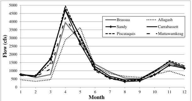
Figure 3-5: Scaled (by DA) Brassua mean annual inflow hydrograph and Scaled (by DA) mean annual inflow hydrographs for reference records. ... 79
Figure 3-6: Brassua mean annual inflow hydrograph and Scaled (by DA) mean annual inflow hydrographs for reference records. ... 80
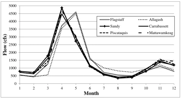
Figure 3-7: Flagstaff mean annual inflow hydrograph and Scaled (by annual inflow) mean annual inflow hydrographs for reference records. ... 83
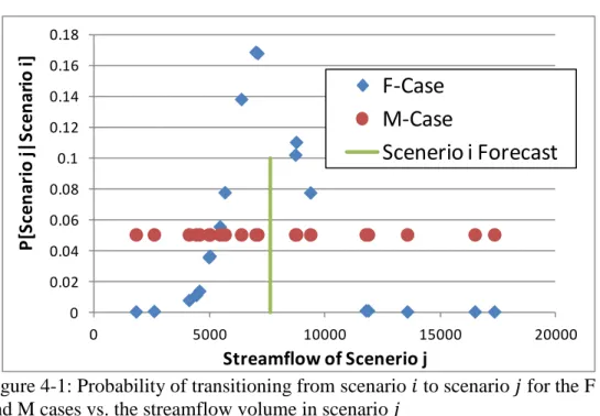
Figure 4-1: Probability of transitioning from scenario to scenario for the F and M cases vs. the streamflow volume in scenario ... 100
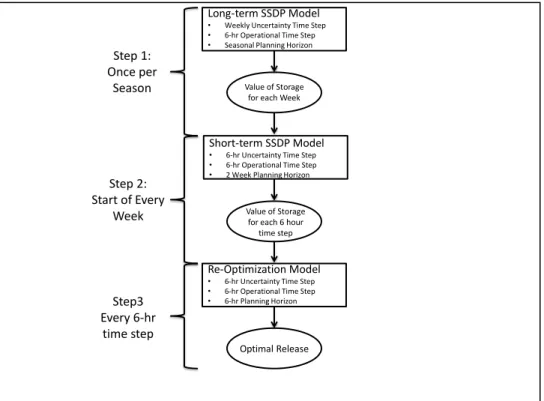
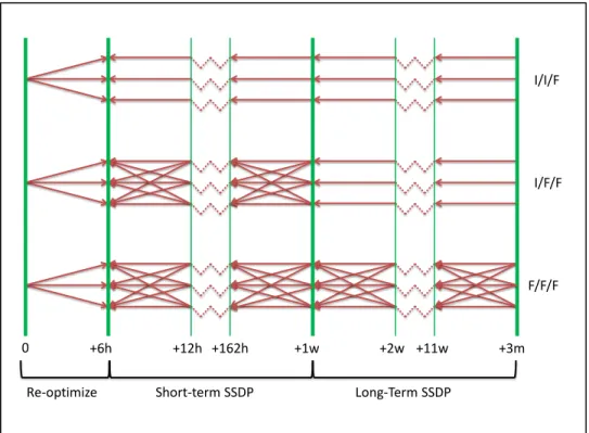
Figure 4-2: Structure of the Proposed Adaptive Time Step SSDP Model ... 106
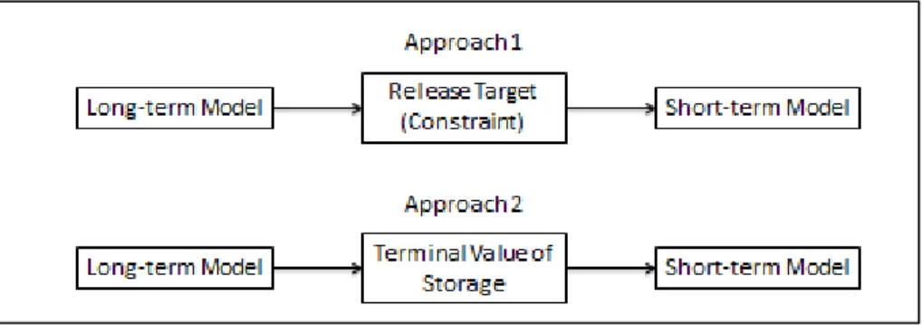
Figure 4-3: Alternative approaches to time decomposition for reservoir operations models. ... 110
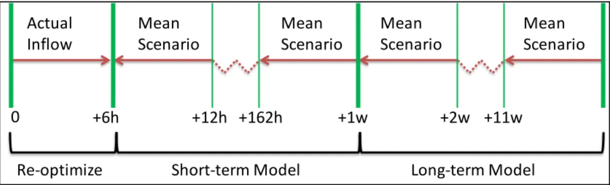
Figure 4-4: Uncertainty structures from various configurations of the time decomposition algorithm. ... 112
Figure 4-5: Schematic of a Hypothetical Single Reservoir System ... 116
Figure 4-6: Range of the vs. of the test systems considered. ... 117
Figure 4-7: Price profile versus generation ... 118
Figure 4-8: Structure of the RCO algorithm ... 120
Figure 4-9: PR for (Big, 8300) system for various algorithms, mean price scheme. 122 Figure 4-10: for (Big, 8300) system for various algorithms, mean price scheme. ... 122
Figure 4-11: for Big reservoirs with varying turbine capacity for various algorithms, mean price scheme. ... 123
Figure 4-12: for (Big, 8300) system for select algorithms, mean price scheme 124 Figure 4-13: for Small reservoirs with varying turbine capacity for various re-optimization forecast precision, mean price scheme. ... 125
Figure 4-14: for Mid reservoirs with varying turbine capacity for various re-optimization forecast precision, mean price scheme. ... 125
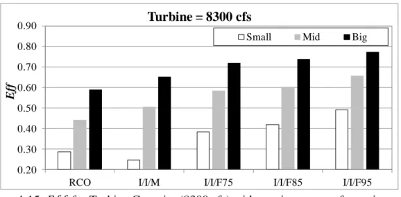
Figure 4-15: for Turbine Capacity (8300 cfs) with varying storage for various algorithms, mean price scheme. ... 126
Figure 4-16: of uncertainty models with increasing sophistication, for system (Big, 8300) and forecast precision , ‗mean price‘ scheme. ... 127 Figure 4-17: of uncertainty models with increasing sophistication, for system (Big,3500) and forecast precision , ‗mean price‘ scheme. ... 128 Figure 4-18: Least sophisticated uncertainty model which matches the of
sophisticated F/F/F uncertainty model, ‗mean price‘ scheme, forecast precision
. ... 129 Figure 4-19: for Mid reservoirs with varying turbine capacity for various re-optimization forecast precision, variable price scheme. ... 130 Figure 4-20: for Turbine Capacity (8300 cfs) with varying storage for various algorithms, variable price scheme. ... 132 Figure 4-21: for (Big, 8300) system for several algorithms, variable price scheme. ... 132 Figure 4-22: for (Small, 2000) system for several algorithms, variable price scheme. ... 133 Figure 4-23: Least sophisticated uncertainty model which matches the of
sophisticated F/F/F uncertainty model, ‗variable price‘ scheme, forecast precision
. ... 134 Figure 4-24: The effect of forecast precision and reservoir size on for stochastic programming models, with fixed turbine capacity (2000 cfs), ‗mean price‘ scheme. 144 Figure 4-25: The effect of forecast precision and reservoir size on for stochastic programming models, with fixed turbine capacity (3500 cfs), ‗mean price‘ scheme. 144 Figure 4-26: The effect of forecast precision and reservoir size on for stochastic programming models, with fixed turbine capacity (5000 cfs), ‗mean price‘ scheme. 144 Figure 4-27: The effect of forecast precision and reservoir size on for stochastic programming models, with fixed turbine capacity (8300 cfs), ‗mean price‘ scheme. 145 Figure 4-28: The effect of forecast precision and turbine capacity on for
stochastic programming models, with fixed storage capacity (Small), ‗mean price‘ scheme. ... 145 Figure 4-29: The effect of forecast precision and turbine capacity on for
stochastic programming models, with fixed storage capacity (Mid), ‗mean price‘ scheme. ... 146 Figure 4-30: The effect of forecast precision and turbine capacity on for
stochastic programming models, with fixed storage capacity (Big), ‗mean price‘ scheme. ... 146 Figure 4-31: The effect of forecast precision and reservoir size on for stochastic programming models, with fixed turbine capacity (2000 cfs), ‗variable price‘ scheme. ... 149
Figure 4-32: The effect of forecast precision and reservoir size on for stochastic programming models, with fixed turbine capacity (3500 cfs), ‗variable price‘ scheme.
... 149
Figure 4-33: The effect of forecast precision and reservoir size on for stochastic programming models, with fixed turbine capacity (5000 cfs), ‗variable price‘ scheme. ... 150
Figure 4-34: The effect of forecast precision and reservoir size on for stochastic programming models, with fixed turbine capacity (8300 cfs), ‗variable price‘ scheme. ... 150
Figure 4-35: The effect of forecast precision and turbine capacity on for stochastic programming models, with fixed storage capacity (Small), ‗mean price‘ scheme. ... 150
Figure 4-36: The effect of forecast precision and turbine capacity on for stochastic programming models, with fixed storage capacity (Mid), ‗mean price‘ scheme. ... 151
Figure 4-37: The effect of forecast precision and turbine capacity on for stochastic programming models, with fixed storage capacity (Big), ‗mean price‘ scheme. ... 151
Figure 5-1: 3-dimensional projection of a 4-dimensional lattice with 10 discrete points evaluated in each dimension. ... 164
Figure 5-2: Quadratic Test Function ... 173
Figure 5-3: Interpolating Gaussian RBF surface ( ) with 9 grid points ... 174
Figure 5-4: Interpolating Gaussian RBF surface ( ) with 9 grid points ... 175
Figure 5-5: Interpolating Gaussian RBF surface ( ) with 9 grid points ... 175
Figure 5-6: Interpolating Gaussian RBF surface ( ) with 9 grid points ... 175
Figure 5-7: Interpolating RBF cubic Spline RBF surface with 9 grid points ... 176
Figure 5-8: Matlab ‗Peaks‘ Function ... 176
Figure 5-9: Interpolating Gaussian RBF ( ) surface for Matlab ‗Peaks‘ with 9 grid points ... 176
Figure 5-10: Interpolating Cubic Spline RBF surface for Matlab ‗Peaks‘ with 9 grid points ... 177
Figure 5-11: Corridor Basis Points before and after Filling. ... 181
Figure 5-12: Corridor Basis Points with Backbone points ... 182
Figure 5-13: Maximum Residual Error ( ) versus Iteration of the Greedy Basis Selection Algorithm ... 184
Figure 5-14: Corridor Basis Points with Backbone after thinning using the Greedy Algorithm, for the easy case ... 185
Figure 5-15: Corridor Basis Points with Backbone after thinning using the Greedy
Algorithm, for the hard case ... 185
Figure 5-16: Schematic of the Kennebec Hydropower System ... 188
Figure 5-17: Schematic of four-reservoir test system used in Section 5.8.2. ... 189
Figure 5-18: SSE in the Corridor Region vs. Number of Basis Points, easy case ... 192
Figure 5-19: Relative RMSE in the Corridor Region vs. Number of Basis Points, easy case ... 192
Figure 5-20: MSE in the Corridor Region vs. Number of Basis Points, hard case ... 198
Figure 5-21: Relative RMSE in the Corridor Region vs. Number of Basis Points, hard case ... 198
Figure 5-22: SSE in Corridor for various RBF functional forms, for two discretization levels, easy case ... 204
Figure 5-23: SSE in Corridor for various RBF functional forms, for two discretization levels with gamma (N = 40/N = 175), hard case ... 205
Figure 5-24: Future Value Function of Corridor DP after one time step (green) and fitted polynomial (red). ... 214
Figure 5-25: Future Value Function of Corridor DP after three time step (green) and fitted polynomial (red) if the sub-optimal termination in Figure 5-23 is ignored. ... 215
Figure 5-26: Future Value Function of Corridor DP after three time step (green) and fitted polynomial (red) if the sub-optimal termination in Figure 5-23 is addressed. . 215
Figure 6-1: Storage Capacity Factor, , versus coefficient of variation for various active storage volumes, . ... 224
Figure 6-2: Powerhouse Flexibility Factor, , versus coefficient of variation for various powerhouse hydraulic capacities, . ... 226
Figure 6-3: vs. Duration ( ) for various reservoir storages (in ) for (in ). ... 235
Figure 6-4: vs. Duration ( ) for various reservoir storages (in ) for (in ). ... 235
Figure 6-5: vs. Duration ( ) for various reservoir storages (in ) for (in ). ... 236
Figure 6-6: vs. Duration ( ) for various reservoir storages (in ) for (in ). ... 236
Figure 6-7: Autocorrelation vs. Lag for daily inflow volume into hypothetical Kennebec reservoir. ... 237
Figure 6-8: Ensemble PSDF of optimal release for System (Big, 2000), , , with the ‗mean-price‘ economic scheme. ... 238
Figure 6-9: Ensemble CPSDF of optimal release and inflow for System (Big, 2000), , , with the ‗mean-price‘ economic scheme ... 239 Figure 6-10: Ensemble PSDF of optimal release for System (Small, 2000),
, , with the ‗mean-price‘ economic scheme. ... 240 Figure 6-11: Ensemble CPSDF of optimal release and reservoir storage for
System (Small, 2000), , , with the ‗mean-price‘ economic scheme. ... 240 Figure 6-12: Ensemble PSDF of optimal release for System (Big, 2000),
, , with the ‗real-price‘ economic scheme. ... 242 Figure 6-13: Ensemble CPSDF of optimal release and inflow for System (Big, 2000), , , with the ‗real-price‘ economic scheme. ... 243 Figure 6-14: Ensemble PSDF of optimal release for System (Big, 8300),
, and , with the ‗real-price‘ economic scheme. ... 244 Figure 6-15: Ensemble CPSDF of optimal release for System (Big, 8300),
, and , with the ‗real-price‘ economic scheme. 244 Figure 6-16: Ensemble PSDF of optimal release for System (Small, 8300),
, and , with the ‗real-price‘ economic scheme. .... 245 Figure 6-17: Ensemble PSDF of optimal release for System (Small, 8300), ‗mean price‘ scheme, 1-week short-term SSDP horizon. ... 246 Figure 6-18: Ensemble PSDF of optimal release for System (Small, 8300), ‗mean price‘ scheme, 2-week short-term SSDP horizon. ... 247 Figure 6-19: Ensemble PSDF of optimal release for System (Small, 2000),
, , with the ‗mean-price‘ economic scheme. ... 251 Figure 6-20: Ensemble PSDF of optimal release for System (Mid, 2000),
, ,with the ‗mean-price‘ economic scheme. ... 251 Figure 6-21: Ensemble PSDF of optimal release for System (Big, 2000),
, , with the ‗mean-price‘ economic scheme. ... 251 Figure 6-22: Ensemble PSDF of optimal release for System (Small, 3500),
, , with the ‗mean-price‘ economic scheme. ... 252 Figure 6-23: Ensemble PSDF of optimal release for System (Mid, 3500),
, , with the ‗mean-price‘ economic scheme. ... 252 Figure 6-24: Ensemble PSDF of optimal release for System (Big, 3500),
, , with the ‗mean-price‘ economic scheme. ... 252 Figure 6-25: Ensemble PSDF of optimal release for System (Small, 5000),
Figure 6-26: Ensemble PSDF of optimal release for System (Mid, 5000),
, , with the ‗mean-price‘ economic scheme. ... 253 Figure 6-27: Ensemble PSDF of optimal release for System (Big, 5000),
, , with the ‗mean-price‘ economic scheme. ... 253 Figure 6-28: Ensemble PSDF of optimal release for System (Small, 8300),
, , with the ‗mean-price‘ economic scheme. ... 254 Figure 6-29: Ensemble PSDF of optimal release for System (Mid, 8300),
, , with the ‗mean-price‘ economic scheme. ... 254 Figure 6-30: Ensemble PSDF of optimal release for System (Big, 8300),
, , with the ‗mean-price‘ economic scheme. ... 254 Figure 6-31: Ensemble CPSDF of optimal release and inflow for System (Small, 2000), , , with the ‗mean-price‘ economic scheme. ... 255 Figure 6-32: Ensemble CPSDF of optimal release and inflow for System (Mid, 2000), , , with the ‗mean-price‘ economic scheme. ... 255 Figure 6-33: Ensemble CPSDF of optimal release and inflow for System (Big, 2000), , , with the ‗mean-price‘ economic scheme. ... 255 Figure 6-34: Ensemble CPSDF of optimal release and inflow for System (Small, 3500), , , with the ‗mean-price‘ economic scheme. ... 256 Figure 6-35: Ensemble CPSDF of optimal release and inflow for System (Mid, 3500), , , with the ‗mean-price‘ economic scheme. ... 256 Figure 6-36: Ensemble CPSDF of optimal release and inflow for System (Big, 3500), , , with the ‗mean-price‘ economic
scheme. ... 256 Figure 6-37: Ensemble CPSDF of optimal release and inflow for System (Small, 5000), , , with the ‗mean-price‘ economic scheme. ... 257 Figure 6-38: Ensemble CPSDF of optimal release and inflow for System (Mid, 5000), , , with the ‗mean-price‘ economic scheme. ... 257 Figure 6-39: Ensemble CPSDF of optimal release and inflow for System (Big, 5000), , , with the ‗mean-price‘ economic scheme. ... 257
Figure 6-40: Ensemble CPSDF of optimal release and inflow for System (Small, 8300), , , with the ‗mean-price‘ economic scheme. ... 258 Figure 6-41: Ensemble CPSDF of optimal release and inflow for System (Mid, 8300), , , with the ‗mean-price‘ economic scheme. ... 258 Figure 6-42: Ensemble CPSDF of optimal release and inflow for System (Big, 8300), , , with the ‗mean-price‘ economic
scheme. ... 258 Figure 6-43: Ensemble CPSDF of optimal release and reservoir storage for
System (Small, 2000), , , with the ‗mean-price‘ economic scheme. ... 259 Figure 6-44: Ensemble CPSDF of optimal release and reservoir storage for
System (Mid, 2000), , , with the ‗mean-price‘ economic scheme. ... 259 Figure 6-45: Ensemble CPSDF of optimal release and reservoir storage for
System (Big, 2000), , , with the ‗mean-price‘ economic scheme. ... 259 Figure 6-46: Ensemble CPSDF of optimal release and reservoir storage for
System (Small, 3500), , , with the ‗mean-price‘ economic scheme. ... 260 Figure 6-47: Ensemble CPSDF of optimal release and reservoir storage for
System (Mid, 3500), , , with the ‗mean-price‘ economic scheme. ... 260 Figure 6-48: Ensemble CPSDF of optimal release and reservoir storage for
System (Big, 3500), , , with the ‗mean-price‘ economic scheme. ... 260 Figure 6-49: Ensemble CPSDF of optimal release and reservoir storage for
System (Small, 5000), , , with the ‗mean-price‘ economic scheme. ... 261 Figure 6-50: Ensemble CPSDF of optimal release and reservoir storage for
System (Mid, 5000), , , with the ‗mean-price‘ economic scheme. ... 261 Figure 6-51: Ensemble CPSDF of optimal release and reservoir storage for
System (Big, 5000), , , with the ‗mean-price‘ economic scheme. ... 261 Figure 6-52: Ensemble CPSDF of optimal release and reservoir storage for
System (Small, 8300), , , with the ‗mean-price‘ economic scheme. ... 262
Figure 6-53: Ensemble CPSDF of optimal release and reservoir storage for System (Mid, 8300), , , with the ‗mean-price‘ economic scheme. ... 262 Figure 6-54: Ensemble CPSDF of optimal release and reservoir storage for
System (Big, 8300), , , with the ‗mean-price‘ economic scheme. ... 262 Figure 6-55: Ensemble PSDF of optimal release for System (Small, 2000),
, , with the ‗real-price‘ economic scheme. ... 263 Figure 6-56: Ensemble PSDF of optimal release for System (Mid, 2000),
, , with the ‗real-price‘ economic scheme. ... 263 Figure 6-57: Ensemble PSDF of optimal release for System (Big, 2000),
, , with the ‗real-price‘ economic scheme... 263 Figure 6-58: Ensemble PSDF of optimal release for System (Small, 3500),
, , with the ‗real-price‘ economic scheme. ... 264 Figure 6-59: Ensemble PSDF of optimal release for System (Mid, 3500),
, , with the ‗real-price‘ economic scheme. ... 264 Figure 6-60: Ensemble PSDF of optimal release for System (Big, 3500),
, , with the ‗real-price‘ economic scheme. ... 264 Figure 6-61: Ensemble PSDF of optimal release for System (Small, 5000),
, , with the ‗real-price‘ economic scheme. ... 265 Figure 6-62: Ensemble PSDF of optimal release for System (Mid, 5000),
, , with the ‗real-price‘ economic scheme. ... 265 Figure 6-63: Ensemble PSDF of optimal release for System (Big, 5000),
, , with the ‗real-price‘ economic scheme. ... 265 Figure 6-64: Ensemble PSDF of optimal release for System (Small, 8300),
, , with the ‗real-price‘ economic scheme. ... 266 Figure 6-65: Ensemble PSDF of optimal release for System (Mid, 8300),
, , with the ‗real-price‘ economic scheme. ... 266 Figure 6-66: Ensemble PSDF of optimal release for System (Big, 8300),
, , with the ‗real-price‘ economic scheme. ... 266 Figure 6-67: Ensemble CPSDF of optimal release and inflow for System (Small, 2000), , , with the ‗real-price‘ economic scheme. ... 267 Figure 6-68: Ensemble CPSDF of optimal release and inflow for System (Mid, 2000), , , with the ‗real-price‘ economic scheme. ... 267
Figure 6-69: Ensemble CPSDF of optimal release and inflow for System (Big, 2000), , , with the ‗real-price‘ economic scheme. ... 267 Figure 6-70: Ensemble CPSDF of optimal release and inflow for System (Small, 3500), , , with the ‗real-price‘ economic scheme. 268 Figure 6-71: Ensemble CPSDF of optimal release and inflow for System (Mid, 3500), , , with the ‗real-price‘ economic scheme. ... 268 Figure 6-72: Ensemble CPSDF of optimal release and inflow for System (Big, 3500), , , with the ‗real-price‘ economic scheme. ... 268 Figure 6-73: Ensemble CPSDF of optimal release and inflow for System (Small, 5000), , , with the ‗real-price‘ economic scheme. 269 Figure 6-74: Ensemble CPSDF of optimal release and inflow for System (Mid, 5000), , , with the ‗real-price‘ economic scheme. 269 Figure 6-75: Ensemble CPSDF of optimal release and inflow for System (Big, 5000), , , with the ‗real-price‘ economic scheme. ... 269 Figure 6-76: Ensemble CPSDF of optimal release and inflow for System (Small, 8300), , , with the ‗real-price‘ economic scheme. 270 Figure 6-77: Ensemble CPSDF of optimal release and inflow for System (Mid, 8300), , , with the ‗real-price‘ economic scheme. ... 270 Figure 6-78: Ensemble CPSDF of optimal release and inflow for System (Big, 8300), , , with the ‗real-price‘ economic scheme. ... 270 Figure 6-79: Ensemble CPSDF of optimal release and reservoir storage for System (Small, 2000), , , with the ‗real-price‘ economic scheme. ... 271 Figure 6-80: Ensemble CPSDF of optimal release and reservoir storage for
System (Mid, 2000), , , with the ‗real-price‘ economic scheme. ... 271 Figure 6-81: Ensemble CPSDF of optimal release and reservoir storage for
System (Big, 2000), , , with the ‗real-price‘ economic scheme. ... 271 Figure 6-82: Ensemble CPSDF of optimal release and reservoir storage for
System (Small, 3500), , , with the ‗real-price‘ economic scheme. ... 272
Figure 6-83: Ensemble CPSDF of optimal release and reservoir storage for System (Mid, 3500), , , with the ‗real-price‘ economic scheme. ... 272 Figure 6-84: Ensemble CPSDF of optimal release and reservoir storage for
System (Big, 3500), , , with the ‗real-price‘ economic scheme. ... 272 Figure 6-85: Ensemble CPSDF of optimal release and reservoir storage for
System (Small, 5000), , , with the ‗real-price‘ economic scheme. ... 273 Figure 6-86: Ensemble CPSDF of optimal release and reservoir storage for
System (Mid, 5000), , , with the ‗real-price‘ economic scheme. ... 273 Figure 6-87: Ensemble CPSDF of optimal release and reservoir storage for
System (Big, 5000), , , with the ‗real-price‘ economic scheme. ... 273 Figure 6-88: Ensemble CPSDF of optimal release and reservoir storage for
System (Small, 8300), , , with the ‗real-price‘ economic scheme. ... 274 Figure 6-89: Ensemble CPSDF of optimal release and reservoir storage for
System (Mid, 8300), , , with the ‗real-price‘ economic scheme. ... 274 Figure 6-90: Ensemble CPSDF of optimal release and reservoir storage for
System (Big, 8300), , , with the ‗real-price‘ economic scheme. ... 274
LIST OF TABLES
Table 3-1: Configurations of ―single-reservoir‖ considered in Chapters 4 and 6 ... 73 Table 3-2: Candidate Reference Records and Target Basin Drainage Area, Mean Annual Inflow Rate, Mean Summer Inflow Rate ... 78 Table 3-3: Summary of proration method used to generate synthetic inflows for Kennebec River ... 82 Table 4-1: Single Reservoir System Configurations ... 116 Table 4-2: Proposed runs for Time Decomposition Model ... 121 Table 4-3: P-values of a two-sided paired t-test of the difference between the
simulated benefits of several algorithms on the (Big, 8300) system. ... 124 Table 4-4: Benefits ( ), Performance Ratio ( ), and Efficiency ( ) for systems with turbine capacity 2000 and ―mean price‖ scheme. ... 147 Table 4-5: Benefits ( ), Performance Ratio ( ), and Efficiency ( ) for systems with turbine capacity 3500 and ―mean price‖ scheme. ... 147 Table 4-6: Benefits ( ), Performance Ratio ( ), and Efficiency ( ) for systems with turbine capacity 5000 and ―mean price‖ scheme. ... 148 Table 4-7: Benefits ( ), Performance Ratio ( ), and Efficiency ( ) for systems with turbine capacity 8300 and ―mean price‖ scheme. ... 148 Table 4-8: Benefits ( ), Performance Ratio ( ), and Efficiency ( ) for systems with turbine capacity 2000 and ―variable price‖ scheme. ... 152 Table 4-9: Benefits ( ), Performance Ratio ( ), and Efficiency ( ) for systems with turbine capacity 3500 and ―variable price‖ scheme. ... 152 Table 4-10: Benefits ( ), Performance Ratio ( ), and Efficiency ( ) for systems with turbine capacity 5000 and ―variable price‖ scheme. ... 153 Table 4-11: Benefits ( ), Performance Ratio ( ), and Efficiency ( ) for systems with turbine capacity 8300 and ―variable price‖ scheme. ... 153 Table 5-1: Basis Functional Forms and Conditions (Regis and Shoemaker, 2007) ... 172 Table 5-2: Greedy Algorithm for basis selection for Interpolating RBF Surface ... 183 Table 5-3: Summary of DP Schemes tested, easy case ... 190 Table 5-4: Summary of DP Schemes tested with flow penalty, hard case ... 197 Table 5-5: Run time and relative RMSE in the Corridor for the 4-reservoir system for various discretization levels for DP with spline and linear interpolation for the easy case ... 200 Table 5-6: Run time and relative RMSE in the Corridor for various discretization levels for DP with spline and linear interpolation for the hard case ... 201
Table 6-1: , , and for projects on the Kennebec, Merrimack and Columbia Rivers. ... 225 Table 6-2: Turbine Capacity and Storage Capacity for each of the 12 system
configurations. ... 232 Table 6-3: Storage Capacity Factor , Storage-days ,
Powerhouse-days , and the Powerhouse Flexibility Factor for twelve system configurations ... 233
CHAPTER 1
INTRODUCTION
The objective in reservoir operations optimization is to select an operating policy which maximizes some objective over a planning horizon. This is a sequential decision problem: the operator must make a decision every month, week, day, or even hour. It is also a stochastic problem: at the time the operator must make a decision there are uncertainties that could affect the consequences of that decision. It can be a consequential problem: environmental and public safety, not to mention profit and recreational benefits could be affected. In some cases it might even be a what Rittel and Webber [1973] call a ‗wicked‘ problem, one which the operator has no right to get wrong: in flooding situations people might die.
In light of these realizations the prospect of designing any optimization tool for planning or managing real-world reservoir systems can seem a daunting task.
However, water resources systems engineers have a long and successful history of applying optimization techniques to real-world decision making [Yeh, 1985; Labadie, 2004,2005]. The research presented in this thesis builds on the body of past work reservoir operations optimization modeling. My thesis has two primary focuses: the representation of streamflow uncertainty in reservoir optimization models, and the reduction of the computational burden of multi-reservoir dynamic programming models.
A fundamental challenge in reservoir operations optimization is that reservoir system is often incentivized to operate in a risky way. The more water that is in
storage the higher the head, and the more energy which is produced per unit volume of water released. Running the reservoir at or near full can be very risky as a sudden inflow could cause a spill, wherein water is not passed through the turbines and generates no energy. Thus the dilemma of the reservoir operator is when and how far to drawdown. To avoid any spill the reservoir might be kept low, but this is inefficient with respect to energy generation. In arid regions like California a large multi-use reservoir might draw down in anticipation of a large storm, but then be unable to refill and meet its irrigation demands later in the summer growing season. Failing to drawdown enough and being forced to spill can be dangerous (particularly at Folsom Dam which is just 15 miles upstream of Sacramento, CA).
One approach to aiding reservoir operators is through the use of dynamic programming (DP) models. Discrete DP (just denoted DP) is an optimization technique which, at each decision point weighs the immediate benefit of a decision immediately taken with the future benefits of a decision made in the future. In
reservoir operation DP weighs the benefit of an immediate release with the benefit of a future release. If the benefits of the immediate release are greater than the benefits of waiting the release is made now, and vice versa. Such models have long been
successfully applied to the reservoir optimization problem [Young, 1967; Hall et al., 1968; Roeffs and Bodin, 1970; Yakowitz, 1982]. Such models can inform operating rules for reservoirs, which give an operator an optimal release based on current reservoir storage. However such models do not take into account the stochasticity of inflows and will not hedge against uncertainty because they implicitly assume that inflows are known with certainty.
Stochastic DP (SDP) is an extension of DP to consider uncertainty in forcings, typically uncertainty in inflow. Remarkably the application of SDP to the reservoir optimization problem pre-dates the simpler deterministic DP, seeing its first use in 1946 by Masse, followed in 1955 by Little. SDP models select optimal releases considering a range of future (and in some cases current) reservoir inflows. Because the future is now uncertain, at each decision point SDP weighs the benefits of an immediate release with the expected benefits of a future release. Typically the distribution of future inflows is modeled as a Markov process where, for example the distribution of flows tomorrow is conditional on the flow today, or the distribution flows today might be modeled as conditional on the flow yesterday [see Yakowitz, 1982 and Loucks et al., 1981]. How the uncertainty in inflows is modeled is a widely studied topic, and is a primary focus of Chapter 4 of this thesis.
How the uncertainty is modeled is important for at least two reasons. First, if the SDP model is to adequately weigh the benefits of future releases, then the
representation of uncertainty must reflect the ability of the decision maker to resolve uncertainty when making future releases. Second, the way in which uncertainty is modeled affects the representation of streamflow, and realistic representation of streamflow persistence is critical if SDP is to properly assess the expected benefits of future releases.
Addressing the first point, Stedinger et al. [1984] shows that improved SDP performance can be achieved be conditioning the distribution of future inflows on a flow forecast. Using this method in an SDP model better reflects the skill of the reservoir operator when making a decision. Using forecasts also potentially improves
the representation of the persistence of flow, which can also improve the performance of SDP models.
Sampling SDP (SSDP) is a variation on SDP that rose largely to address the concern about the representation of inflows in SDP models. In SDP inflows are represented by intact streamflow scenarios which might be historical flows [Kelman et al., 1990; Cote et al, 2011], ensemble forecasts [Faber and Stedinger, 2001; Kim et al., 2007], or they might be climate projections [Vicuna et al., 2010]. In any case the persistence of flow is doubtlessly better represented by time series than Markov
Processes, allowing SSDP to better assess the value of future releases, as demonstrated by Cote at al. [2011].
Like SDP, SSDP considers a range of potential scenarios when selecting a current decision, but unlike SDP, SSDP evaluates the benefits of that decision on an intact scenario. How the uncertainty is represented when SSDP selects an optimal release can have a large impact on the value of the resulting optimal operating policy, as demonstrated by Faber and Stedinger [2001] for a reservoir in Colorado, and later by Kim et al. [2007] for a reservoir in Korea.
Chapter 4 of this thesis extends that work in four ways.
1) It considers much shorter time steps: most previous SSDP studies use weekly time steps, whereas Chapter 4 considers time steps as short as 6-hours. This tests the SSDP methodology for sub-daily operation, a relevant research topic as short-term ensemble forecasts become available.
2) It considers a wide range of systems by fixing the hydrology and drastically changing the storage and turbine capacity. Unlike previous studies which focus on a single system, the analysis in Chapter 4 is able to draw more general conclusions across different categories of reservoirs.
3) It compares operation of the different reservoir systems with different economic models, allowing us to isolate the effects of hydrologic uncertainty and price variability on operations.
4) Finally it utilizes synthetically generated inflow forecasts which have a desired precision which allows the examination of the value of forecast precision on SSDP model performance.
In support of the study in Chapter 4, Chapter 5 of this thesis introduces a number of non-parametric statistics which allow for the classification of reservoir types (i.e. run-of-river, storage only, generating reservoir) regardless of the scale of the reservoir in question. Chapter 4 reports results comparing some of the largest hydropower reservoirs in North America with small reservoirs in Northern Maine, demonstrating that the magnitude of the project alone is not a good indicator of how the project operates or should be modeled. A regression procedure and a spectral analysis procedure which help a modeler determine the critical time scales of operation for a reservoir which can answer the question: do we operate at an hourly, daily, weekly, monthly cycle (or perhaps decadal cycle for Hoover Dam on the
Colorado River). The Spectral analysis approach is novel for water resources systems analysis, and shows great potential as a diagnostic technique.
Dynamic programming models become very computationally difficult to solve in high dimensions, or for the reservoir operations case, for multiple reservoirs. This is a well-documented problem, dating back to Richard Bellman who coined the term the ‗curse of dimensionality‘ in 1961 [Bellman, 1961]. Chapter 2 of this thesis explains in detail who high dimensional problems are difficult in dynamic
programming, and some of the techniques which are commonly used to diminish the ‗curse.‘ Chapter 5 presents a new approach called Corridor DP, which achieves
computational savings by focusing on storage combinations which a multi-reservoir system is most likely to visit. It is shown that the Corridor DP algorithm is more computationally efficient than other traditional DP methods.
Finally Chapter 7 provides some concluding remarks and discussion of planned extensions for the methods presented in this thesis.
REFERENCES
Cote, P., Haguma, D., Leconte, R. & Krauc, S. 2011, "Stochastic Optimization of Hydro-Quebec hydropower installations: a statistical comparison between SDP and SSDP methods", Canadian Journal of Civil Engineering, vol. 38, no. 12, pp. 1427-1434.
Hall, W.A., Butcher, W.S. & Esogbue, A. 1968, "Optimization of the operation of a multiple-purpose reservoir by dynamic programming", Water Resources Research, vol. 4, no. 3, pp. 471.
Kelman, J., Stedinger, J.R., Cooper, L.A., Hsu, E. & Yuan, S. 1990, "Sampling stochastic dynamic programming applied to reservoir operation", Water Resources Research, vol. 26, no. 3, pp. 447-454.
Kim, Y., Eum, H., Lee, E. & Ko, I. 2007, "Optimizing Operational Policies for a Korean Multireservoir System using Sampling Stochastic Dynamic Programming with Ensemble Streamflow Prediction", Journal of Water Resources Planning and Management, vol. 133, no. 1, pp. 4-14.
Labadie, J.W. 2005, "Closure to "Optimal Operation of Multi-Reservoir Systems: State-of-the-Art Review"", Journal of Water Resources Planning and
Management, vol. 131, no. 5, pp. 407.
Labadie, J.W. 2004, "Optimal Operation of Multireservoir Systems: State-of-the-Art Review", Journal of Water Resources Planning and Management, vol. 130, no. 2, pp. 93-111.
Little, J.D.C. 1955, "Use of Storage Water in a hydroelectric System", Journal of Operations Research, vol. 3, pp. 187-197.
Loucks, D.P., Stedinger, J.R. & Haith, D.A. 1981, Water Resources Systems PLanning and Analysis, 1st edn, Prentice-Hall, Englewood Cliffs, N.J.
Masse, P.B.D. 1946, Les Reserves et al Regulation de l'Avenir dans la Vie Economique, Hermann and Cie, Paris.
Rittel, H.W.J. & Webber, M.M. 1973, "Dilemmas in a General Theory of Planning",
Roefs, T.G. & Bodin, L.D. 1970, "Multireservoir operation studies", Water Resources Research, vol. 6, no. 2, pp. 410.
Stedinger, J.R., Sule, B.F. & Loucks, D.P. 1984, "Stochastic dynamic programming models for reservoir operation optimization.", Water Resources Research, vol. 20, no. 11, pp. 1499-1505.
Vicuna, S., Dracup, J.A., Lund, J.R., Dale, L.L. & Maurer, E.P. 2010, "Basin-scale water system operations with uncertain future climate conditions: Methodology and case studies", Water Resources Research, vol. 46, no. W04505, pp. 1-19.
Yakowitz, S. 1982, "Dynamic programming applications in water resources", Water Resources Research, vol. 18, no. 4, pp. 673-679.
Yeh, W.W. 1985, "Reservoir Management and Operations Models: A State-of-the-Art Review", Water Resources Research, vol. 21, no. 12, pp. 1797-1818.
Young, G.K. 1967, "Finding reservoir operating rules", Journal of Hydraulics Division American Society of Civil Engineers, vol. 93, no. HY6, pp. 297.
CHAPTER 2
A REVIEW OF DYNAMIC PROGRAMMING MODELS FOR HYDROPOWER OPTIMIZATION
This chapter provides a brief introduction to dynamic programming techniques commonly applied to reservoir operations optimization problems, along with a short history and literature review on the topic. Dynamic programming algorithms have found widespread application across a variety of fields including natural resource economics [Insley and Rollins, 2005; Dixit, 1990; Conrad and Clark, 1987], product distribution networks [Topaloglu and Kunnumkal, 2006], power system control [Yu et al., 2014], and of course water resources systems analysis to name a few. This chapter will focus on application to reservoir operations problems and will primarily focus on the issues of uncertainty representation and efficient high-dimensional dynamic programming for reservoir problems. For a broader discussion of reservoir
optimization and dynamic programming applied to water resources see Labadie [2004, 2005], Yeh [1985], and Yakowitz [1982]. For a more in-depth discussion of the dynamic programming more broadly Powell [2007] and Bertsekas [2011] are excellent reference sources. Section 2.1 introduces dynamic programming and stochastic
dynamic programming for reservoir operations problems. Section 2.2 introduces and describes the use of sampling stochastic dynamic programming algorithms. Section 2.3 is a brief narrative describing the evolution of DP and SDP methods in water resources systems analysis since the mid-1950s. Section 2.4 provides particular discussion on the areas of DP and SDP which addressed in Chapters 4 and 5, and finally Section 2.5 includes some concluding remarks.
Section 2.1 Dynamic Programming and Stochastic Dynamic Programming
Operation of a reservoir system requires the operator to select a series of releases which satisfy a host of constraints and hopefully maximize the value of some objective or set of objectives. This is a challenging problem because system forcing, both hydrologic and economic, are uncertain at the time a decision must be made. As the system responds to forcings and to actions taken by the operator, its state will evolve and present new optimization problem each time an action must be taken. Further complicating the problem, objectives and constraints are often non-linear in reservoir systems, rending many mathematical solution techniques inadequate.
Dynamic Programming (DP) and Stochastic DP (SDP) are well suited to this type of problem. They impose virtually no restriction on the functional form of the objective and constraints of a problem, and they provide a dynamic operating rule that accounts for the evolution of the system in response to an operator‘s control and in the case of SDP to realizations of random forcing variables.
The DP framework assumes a simple additive model of reservoir system benefits over a planning horizon (equation (2-1)). In each discrete time a decision (a release for reservoirs), , must be made. The incremental benefit of , , also depends on the current reservoir storage, , and the current inflow . It is assumed that at the end of the planning period (index ) storage reaming in the reservoir has some terminal value, ( ).
∑ ( )
( ) (2-1)
The evolution of the reservoir system in response to the operator‘s decision is given by
( ) (2-2)
where is an evaporation/seepage loss term. The challenge of the operator is to pick the best series of releases or equivalently the best sequence of reservoir storages over the planning period .
Because of the assumption of sequential evolution of the system state and the additive benefit function DP can be used to solve this planning problem. The DP solution to the planning problem posed by equations (2-1) and (2-2) is given by:
( ) * ( ) ( ) * +
( ) (2-3)
where and ( ). The traditional solution technique for the DP model is start with ( ), and to solve equation (2-3) recursively backwards in time until one arrives at present time and has ( ) [Bellman, 1957]. The result of the DP solution process is a decision rule which specifies an optimal for any and future value function of water in storage ( ) for each time step in the in the planning period. In the DP formulation in equation (2-3) the current storage is the state-variable, meaning that the state of the reservoir system is fully described by . In multiple reservoir DP models it is common to assign a storage state to each reservoir, so would become a -dimensional vector.
SDP is a natural extension of the DP framework to consider the stochastic nature of the forcings such as the inflows . Given a description of the stochastic forcings, one must compute the expected benefits associated with each decision . To describe the hydrologic state of the basin, it is common to add a hydrologic state variable. A simple hydrologic state variable might be the previous or current period‘s
inflow, . If one then assumes that the is known in time [as in Loucks et al., 1981 and Tejada et al., 1995] one obtains the model.
( ) { ( )
, ( )-}
* +
(2-4)
Here the expected future benefits are computed with the probability
, -, which is the probability of the next period‘s flow given the flow in the
current period. Many papers have explored alternative hydrologic states including snow-water equivalent or antecedent soil moisture [Cote et al., 2011] or an inflow forecast [Stedinger et al., 1984, Kelman et al., 1990; Maceira and Kelman, 1991; Karamouz and Vasiliadis, 1992; Tejada et al., 1995; Kim and Palmer, 1997; and Kim et al., 2007]. Computing correct transition probabilities based on flow forecasts is described at length in Chapter 4 of this thesis. An SDP model which uses a generic is given by equations (2-5) and (2-6):
( )
, ( ) ( and * +
(2-5)
{ * + ( ( ))} (2-6)
where is the maximum reservoir storage level and is the optimal target
release in time . The distinction between and is necessary because may not be feasible because is no longer known. Equation (2-6) ensures that the final selected is feasible. It should be noted that multiple hydrologic states might be employed. For example Karamouz and Vasiliadis [1992] assign a state variable to the current inflows and a state variable to the next period‘s inflows. Tejada [1993]
information from several previous days‘ flows can be leveraged into a single
hydrologic state variable. Chapter 4 describes in great detail how one might generate the needed probabilities to compute
if is a vector of hydrologic (or economic)
states.
The backwards recursive DP and SDP procedure described above provides an optimal policy for each system state at discrete time steps over the planning period. To develop these policies numerically the storage state space is often discretized, and the ―optimal‖ policy is computed for each discrete state at each time.
When implementing the numerically derived policy, the reservoir is unlikely to reside only in the discrete points which happened to have been sampled, and will more likely fall between the discrete points. One solution to this problem is to interpolate within the policy table, or to fit some simple function to that table. Another approach is re-optimization which selects an optimal release given the current state by
performing a one-step SDP optimization with the current reservoir conditions (Tejada et al., 1993). Equation (2-7) describes the re-optimization step.
{ ( )
, ( )-}
(2-7) where is the current hydrologic information. Tejada et al. [1993] compared the performance of models which interpolate in the policy table to select an optimal release and models which use re-optimization. They found that re-optimization
generally results in better operation, particularly when coarse grids were used in the initial backwards moving that derived the future value function. Furthermore they found that use of re-optimization improved the reliability of meeting both energy and
water targets. Re-optimization is used when implementing optimal policies derived from sampling SDP models in Chapter 4.
Section 2.2 Sampling Stochastic Dynamic Programming
SDP models often overestimate the benefits actually attainable with particular release decisions because decisions are evaluated with the same simplified streamflow description used in developing the SDP policy [Tejada et al., 1993]. This has led to the develop of sampling SDP models. SSDP represents future streamflow with an ensemble of scenarios, which are time series of reservoir inflow and other variables (like energy price). This provides a discrete description of streamflow that implicitly captures the joint distribution of streamflow, forecasts, and other variables across time and space, without requiring an explicit probability distribution [Kelman et al., 1990; Faber and Stedinger, 2001; Kim et al., 2007; Vicuna et al., 2011;Eum et al., 2011;Cote et al., 2011].
Kelman et al. [1990] present a SSDP model for optimizing hydropower operation for a system in California. Their model (equations (2-8) and (2-9)) takes reservoir storage, , inflow forecast, , and the current scenario trace as state
variables (i.e. the hydrologic state, , is described by both a forecast and a scenario). Their SSDP formulation is given by:
, ( ( ) * , ( * + (2-8) ( ) ( ( ) ) , ( )- (2-9)
* +
where ( ) is the reservoir inflow in time and scenario , and is a flow forecast in time .
Equation (2-8) is the Decision Model which is used to select an optimal and equation (2-9) is the Simulation Model which is used to assess the benefits of the optimal release. This the key difference between SSDP and SDP: SDP uses the same model to select an optimal release and assess its benefit (for example equation (2-5)). The Decision Model considers possible transitions between scenario traces, whereas the Simulation Model simulates the operational benefits on a single intact scenario, thus preserving the persistence of hydrologic inflows. To numerically solve this SSDP model, equations (2-8) and (2-9) must be solved for each discrete pair of
( ), for each trace , for every time step in the planning period.
The double expectation in equation (2-8) captures both the probability of a future forecast given the current forecast and an inflow, and the transition probability of a future scenario given the current forecast. Faber and Stedinger [2001] avoid the need for a double expectation and a forecast state variable by utilizing the historical forecast series associated with each trace. Thus the forecast state variable is
embedded in the scenario state variable, and the scenario state variable becomes the sole hydrologic state variable. This allows a very large reduction in the computational demands of the solution algorithm by reducing the dimension of the implicit
hydrologic state variable (going from and to just use of which has an with it). A reasonable concern is if all combinations of and were reasonable, or likely. In many cases the answer is that some were not likely, and thus the modeling process
was not efficient. For single reservoir systems such as that considered by Kelman et al. [1990], this is not particularly important. However, as we strive to model multiple reservoir systems, economy in the computational algorithm becomes much more important. The corridor model explored in Chapter 5 addresses this issue. The Faber and Stedinger [2001] SSDP formulation is:
{ ( ( ) , ( )-} * + (2-10) ( ) ( ( ) ) ( ) * + (2-11)
where equation (2-10) is the SSDP Decision Model and equation (2-11) is the SSDP Simulation Model. This is the SSDP formulation which is adopted in this study. To compute
, the probability , - is needed. The computation of these probabilities
is discussed in great detail in Chapter 4. Faber and Stedinger [2001] and Kim et al. [2007] used ESP forecasts and historical inflows as SSDP traces, whereas Kelman et al. [1990] and Cote et al. [2011] use only historical flows. Vicuna et al. [2011] used climate scenarios from different GCM results with different greenhouse gas scenarios as SSDP traces.
Section 2.3 The Evolution of SDP Algorithms for Reservoir Optimization
The name ‗Dynamic Programming‖ is somewhat of a misnomer in that it is not programming in the same way that linear programming is a solution method for a subset of optimization models. Rather, DP is a theory of multi-stage decision processes: it is a way of modeling a decision process, which might be solved by any number of programming methods, including linear programming models (see Loucks,
1968 for just one example). Richard Bellman, the father of DP, later regretted the name ―Dynamic Programming,‖ but explained the choice was influenced by a desire to make the new theory sound interesting to funding agencies in a time when great advances in linear programming were taking place [Bellman, 1989].
Yakowitz [1982] and Esogbue [1989] see the solution of water resources problems as a major impetus for the early development of DP methods. In fact, Bellman‘s foundational book on DP [Bellman, 1957] prominently features a water resources problem. Yakowitz [1982] sees water resources as an ideal laboratory for the development of DP methods. Yakowitz [1982] and Esogbue [1989] are concerned with DP applied to water resources problems in general, whereas this section will focus on DP for reservoir problems.
The first application of an SDP model to reservoir operations was
demonstrated by Masse [1946]. The earliest example in the English literature is Little [1955]. That work considers the optimal operation of a single reservoir for
hydropower, and provided the prototypical SDP formulation for much of the later work in SDP for reservoirs [Yakowitz, 1982]. Little‘s model used a Markov description of reservoir inflow wherein the distribution of the current inflow is
conditioned on the value of the previous period‘s inflow. Thus, the state of the single reservoir system is described by a storage state and a hydrologic state (previous period‘s inflow). Little applied his SDP model to the operation of Grand Coulee Dam on the Columbia River. Interestingly, he found that simulated operation using a policy derived by the SDP model resulted in only a 1% performance over existing rule curve
policies. The study described in Chapter 4 of this thesis experienced similar gains, and develops appropriate metrics for comparison of algorithms.
Gessford and Karlin [1958] considered and SDP model for a single reservoir wherein the inflows are independent, so a hydrologic state variable is not required. This analysis allowed them to derive more general optimal operating strategies using inventory theory. Russell [1972] extended this work to include penalties on releases. The value of this work is that it allows one to draw general conclusions about optimal reservoir operating behavior. Whether the assumption of independently distributed inflows is valid depends on the time step of the model and the hydrology of the
system. Buras et al. [1963] adopt such an approach in a study of the joint operation of a reservoir and aquifer with a monthly time step. Other early examples include Askew [1974a,b, 1975] and Rossman[1977].
Loucks [1968] presents steady-state SDP models, along with equivalent linear programming (LP) formulations. Those models used either the current inflow or the previous period‘s inflow as hydrologic states. Similarly, Loucks and Faulkson [1970] and Butcher [1971] present SDP models which derive a steady state optimal policy, with a hydrologic state variable. Loucks and Gablinger [1970] provide an SDP and equivalent LP formulation to solve for the optimal policy in the transient case with discounting.
Su and Deininger [1974] apply an SDP model the operation of Lake Superior, using a hydrologic state variable of the previous period‘s inflow, which is represented as a Markov process. To reflect seasonal variations in hydrologic conditions the
transition probabilities of the Markov process in that formulation are transient, whereas most previous applications considered stationary Markov models of inflow.
Subsequent improvements in SDP models resulted from the use of better hydrologic information as a state variable. Bras et al. [1983] showed that
incorporation of current hydrologic forecast information in an SDP model can lead to more efficient operations in a study of the High Aswan Dam. Revisiting the High Aswan Dam problem, Stedinger et al. [1984] incorporated available hydrologic information into the SDP decision model by using the inflow forecast as the hydrologic state variable. The resultant steady-state operating policy allowed
decisions to depend on current forecasts without the need to re-formulate and re-solve a new SDP at each time step. Tejada et al. [1995] illustrated the use of forecasts in an SDP model of reservoirs in the Central Valley of California. Turgeon [2005] illustrates the advantages of a comparable algorithm. Similarly Krzystofowicz and Watada [1986], Krzystofowicz and Reese [1991], and Krzystofowicz [1999] develop a
description of forecast-streamflow uncertainty that employs Bayesian decision theory. Karamouz and Vasiliadis [1992] and Kim and Palmer [1997] explored the use of such Bayesian SDP models. Kelman et al. [1989, 1990], Faber [2000], Faber and Stedinger [2001], Kim et al. [2007], Cote et al. [2011], and Eum et al. [2011] focus on better descriptions of the joint distribution of flows and forecasts using sampling SDP (SSDP).
Kelman et al. [1989;1990] introduced sampling SDP to optimize water systems operations on the Feather River in California, using multiple historical time-series as scenarios to capture by example the variability of streamflow processes. A scenario is
defined here as a streamflow hydrograph and the associated volume forecast time-series and energy market parameters and loads. In this case the hydrologic state variable is the set of streamflow scenarios.
If the probabilities assigned to historical streamflow series are appropriately conditioned on historical volume forecasts as described by Kelman et al. [1990] and Faber and Stedinger [2001], many historical streamflow series may be extremely unlikely, in effect reducing the number of relevant streamflow scenarios available to compute the expected future value of water in storage. This is identified by Labadie [2004] as a primary drawback of SSDP.
It would seem then to be better to use sets of streamflow series that are consistent with anticipated basin flows. The National Weather Service‘s Ensemble Streamflow Prediction (NWS ESP) procedure produces streamflow forecasts in the form of multiple hydrographs, each a possible realization of seasonal streamflow [Day, 1985; Schaake and Larson, 1998]. Because such hydrographs are often derived from historical weather sequences, historical (or modified historical) energy market signals could very easily be embedded in the ESP forecasts. Such sets of hydrographs (and other embedded signals) capture by example the temporal and spatial correlation structure of the streamflow series. One advantage of using SSDP algorithms with ESP for multiple reservoir optimization is that the ESP captures the interrelationships among streamflows in those basins by utilizing historical weather patterns for different years [ Faber, 2000; Faber and Stedinger, 2001]. Faber and Stedinger [2001]
recently Kim et al. [2007] and Eum et al. [2011] demonstrate the use of ESP forecasts for basins in Korea.
Askew [1974a, b, 1975] introduced chance-constrained SDP in which
probability of failure to meet some constraint must be less than a prescribed level, . Yakowitz [1982] points out that Askew‘s approach satisfies the chance constraint, but is not guaranteed to be the optimal policy satisfying that constraint. Sneidovich and Davis [1975] propose adding as a state variable for the chance constrained SDP model, with added conditions for the chance constraint. Askew [1974b] proposes a variation on chance constraints in which the expected number of constraint violations is bounded. Rossman [1977] presents an approach for solving such a model based in Lagrangian duality theory. If a state variable is added for the number of failures, then Rossman‘s expectation constraints are equivalent to probabilistic constraints
[Sneidovich,1979].
The previous discussion in this section has focused nearly exclusively on single-reservoir applications of SDP. Solution of multi-reservoir SDP and DP models is more difficult, and was somewhat more limited in early applications of SDP for reservoir optimization. Section 2.4.2 discusses solution techniques for reducing the burden of multi-reservoir optimization and Chapter 5 of this thesis presents new developments in this area. The first SDP model for multiple reservoirs was presented by Schweig and Cole [1968], who consider a two reservoir system. Yakowitz [1982] points out that their model is essentially the same as the joint reservoir-aquifer model developed by Buras [1963]. Roefs and Bodin [1970] and Heidari et al. [1971] provide early examples of multi-reservoir deterministic DP models. Because deterministic DP
models do not include a hydrologic state variable, the number of reservoirs included in early studies was generally greater for deterministic DP models compared to stochastic DP models. In fact a four reservoir deterministic DP model is presented as early as Larson [1968], and a 10-reservoir deterministic DP model is solved using ‗constrained differential dynamic programming‘ by Murray and Yakowitz [1979]. Pereira and Pinto [1985] solve a 39 reservoir problem using stochastic dual dynamic
programming. This and other methods for solving DP and SDP models for large systems are described in more detail in Section 2.4.2.
Section 2.4 Special Concerns addressed in this Thesis
Chapter 4 of this thesis is concerned with the representation of uncertainty in reservoir optimization models and the value of forecasts to hydropower operation. Section 2.4.1 provides an overview of previous work in this area. Chapter 5 of this thesis develops a new method to cope with the curse of dimensionality. Section 2.4.2 provides a brief overview of previous efforts to address the curse of dimensionality for multi-reservoir dynamic programming models.
Section 2.4.1 Representations of Uncertainty
How uncertainty is represented in a reservoir optimization model can have a major impact on the quality of the resulting ‗optimal decision‘ [Tejada-Guibert et al., 1995]. One might intuitively guess that the more complex the model, the more
hydrologic information included, the better the resulting decisions, but Klemes [1977] reminds us that this often is not so. Precisely how uncertainty should be modeled in SDP models for reservoirs has remained an active area of research since SDP models were first applied to the reservoir optimization problem.