Predicting Stock Markets with Neural Networks

Predicting Stock Markets with

Neural Networks

A Comparative Study

Torkil Aamodt

Predicting Stock Markets with Neural

Networks

Torkil Aamodt May 4, 2015

Abstract

Correctly predicting price movements in stock markets carries obvious economical benefits. The task is traditionally solved by analyzing the underlying company, or the historical price development of the company’s stock. A third option that is undergoing active research is to create a predictive model of the stock using machine learning. This thesis follows the latter approach, in which a machine learning algorithm is presented with historical stock data. The algorithm uses this information to train a model that is expected to infer future prices given recent price information. Machine learning is a large field within computer science, and is under constant development. Breakthroughs in a family of machine learning models known as artificial neural networks have spiked an increased interest in these models, including applying them for financial prediction. With a plethora of models available, selecting between them is difficult, especially considering the constant flow of emerging models and learning techniques.

This study compares a selection of artificial neural networks when applied for stock market price prediction. The networks are selected to be relevant to the problem, and aim at covering recent advances in the field of artificial neural networks. The networks considered include: Feed forward neural networks, echo state networks, conditional restricted Boltzmann machines, time-delay neural networks and convolutional neural networks. These models are also compared to another type of machine learning algorithm, known as support vector machines. The models are trained on daily stock exchange data, to make short-term predictions for one day and two days ahead. Performance is evaluated in the context of following the models directly in a financial strategy, trading every prediction they make. Additional performance measures are also considered, to make the comparison as informed as possible.

Possibly due to the noisy nature of stock data, the results are slightly inconsistent between different data sets. If performance is averaged across data sets, the feed forward network generates most profit during the three year test period: 23.13% and 30.43% for single-step and double-step prediction, respectively. Convolutional networks get close to the feed forward in terms of profitability, but are found unreliable due to their unreasonable bias towards predicting positive price changes. The support vector machine delivered average profits of 17.28% for single-step and 11.30% for double-step. Low profits or large deviations were observed for the other models.

Preface

The efforts associated with writing this thesis have challenged me in sev-eral aspects. Finding my way through the jungle of neural network re-search and applying the models demanded my full attention. Furthermore, writing a thesis is an endeavor by itself. There are a number of people that have contributed to the completion of this thesis.

I would like to thank my supervisor at BEKK, Jørgen Braseth. Our discussions surrounding direction of the research, as well as his genuine comments regarding my progress, have kept me focused and motivated throughout the work. I would also like to thank Professor Jim Tørresen, my supervisor at the university. His feedback on the thesis and continuous support has been tremendously helpful to me during the course of my work.

Professor Herman Ruge Jervell initially functioned as my university supervisor, and I am grateful for his efforts and advices. A discussion with associate professor Dag Einar Sommervoll enriched my perspective on the task, which led to the inclusion of information regarding the day of week in the data samples.

Finally, I thank my family and friends, who have been nothing but supportive and understanding of my preoccupied state. I especially thank my sister Yngvild, who generously spent her own free time to read through and comment the entire thesis.

Contents

1 Introduction 1 1.1 Motivation . . . 1 1.1.1 Stock Markets . . . 1 1.1.2 Machine Learning . . . 2 1.2 Problem Formulation . . . 3 1.3 Related Work . . . 4 1.4 Outline . . . 4 1.4.1 Background . . . 4 1.4.2 Methodology . . . 5 1.4.3 Experiments . . . 5 1.4.4 Conclusion . . . 5 1.4.5 Future Work . . . 5 2 Background 7 2.1 Stock Markets . . . 7 2.1.1 Stock Exchanges . . . 7 2.1.2 Market Positions . . . 8 2.1.3 Indices . . . 8

2.1.4 Stock Market Data . . . 9

2.2 Machine Learning . . . 11

2.2.1 Sample Data . . . 11

2.2.2 Supervised Learning . . . 12

2.2.3 Unsupervised Learning . . . 12

2.2.4 Connectivity . . . 12

2.2.5 Output Semantics and Problem Space . . . 13

2.2.6 Hyper-parameters . . . 13 2.2.7 Separability . . . 14 2.2.8 Data Fitting . . . 14 2.3 Neural Networks . . . 15 2.3.1 Biological Inspiration . . . 16 2.3.2 Artificial Adaption . . . 17 2.3.3 Backpropagation . . . 20 2.3.4 Deep Learning . . . 23 2.4 Supervised Models . . . 23

2.4.1 Recurrent Neural Network . . . 24

2.4.2 Echo State Network . . . 25

2.4.4 Convolutional Neural Network . . . 28

2.4.5 Support Vector Machine . . . 29

2.5 Unsupervised Models . . . 32

2.5.1 Restricted Boltzmann Machine . . . 32

2.5.2 Conditional Restricted Boltzmann Machine . . . 35

2.5.3 Deep Belief Network . . . 36

3 Methodology 39 3.1 Challenges . . . 39 3.2 Test Scenario . . . 40 3.2.1 Implementation Notes . . . 40 3.2.2 Tuning Hyper-parameters . . . 43 3.2.3 Training . . . 44 3.2.4 Evaluating . . . 44 3.3 Data . . . 46 3.3.1 Data Selection . . . 46 3.3.2 Granularity . . . 50 3.3.3 Preprocessing . . . 51

3.3.4 Adjusting for Splits . . . 53

3.4 Models . . . 53

3.4.1 Support Vector Regression . . . 53

3.4.2 Feed Forward Neural Network . . . 54

3.4.3 Echo State Network . . . 54

3.4.4 Conditional Restricted Boltzmann Machine . . . 55

3.4.5 Time-Delay Neural Network . . . 56

3.4.6 Convolutional Neural Network . . . 56

3.5 Limitations . . . 57

3.5.1 Limited Depth . . . 57

3.5.2 Simplified Profit Estimation . . . 58

4 Experiments 59 4.1 How to Read the Results . . . 59

4.1.1 Performance Plots . . . 59

4.1.2 Aggregated Results . . . 60

4.1.3 Textual Description . . . 61

4.2 Results . . . 61

4.2.1 Support Vector Regression . . . 61

4.2.2 Feed Forward Neural Network . . . 63

4.2.3 Echo State Network . . . 66

4.2.4 Conditional Restricted Boltzmann Machine . . . 68

4.2.5 Time-Delay Neural Network . . . 70

4.2.6 Convolutional Neural Network . . . 72

4.3 Analysis . . . 74

4.3.1 Index Performance . . . 75

4.3.2 Stock Performance . . . 77

4.3.3 CNN Bull Ratio . . . 79

4.3.4 Mean Squared Error Performance . . . 79

4.3.6 Large Deviations . . . 80

4.3.7 Supervised or Unsupervised . . . 80

4.3.8 Value as a Trading Strategy . . . 80

4.3.9 Average Profits . . . 81

4.3.10 Single-step vs. Double-step . . . 82

5 Conclusion 83 6 Future Work 85 6.1 Ensemble Modeling . . . 85

6.2 Enhance Training Samples . . . 85

6.3 Analyze Feature Detectors . . . 86

Acronyms

ANN Artificial Neural Network. 2–4, 11–16, 18–20, 39, 40, 53, 80, 83

ARIMA Autoregressive Integrated Moving Average. 4

BAC Bank of America Corporation. xiii, 40, 47–49, 61, 63, 64, 66, 68, 70, 72, 74, 77, 80, 83–85

BPTT Backpropagation Through Time. 24, 25, 54

CD Contrastive Divergence. 34, 36

CNN Convolutional Neural Network. viii, xiii, xv, 16, 23, 28, 29, 40, 41, 43, 56, 57, 72–81, 83, 84

convRBM Convolutional Restricted Boltzmann Machine. 41

CRBM Conditional Restricted Boltzmann Machine. viii, xiii, xv, 3, 4, 12, 16, 35, 40, 42–44, 55, 56, 68–70, 75–81, 83

DBN Deep Belief Network. viii, 4, 16, 36, 37, 80

ESN Echo State Network. vii, viii, xiii, xv, 4, 16, 25, 26, 40, 43, 44, 54, 55, 57, 66–68, 75–79, 81, 83

FFNN Feed Forward Neural Network. viii, xiii, xv, 3, 4, 13, 16, 18, 23, 24, 26–29, 32, 34, 40, 43, 54, 63–66, 75–81, 83, 84

GPU Graphics Processing Unit. 22

GSPC S&P 500. xiii, 40, 43, 46–48, 54, 61, 63, 64, 68, 70, 72, 74, 75, 77

HMM Hidden Markov Model. 3

IXIC NASDAQ Composite. xiii, 40, 46–48, 61, 63, 64, 68, 70, 72, 74, 77, 78

kNN k-Nearest Neighbors. 12–14

MNIST Mixed National Institute of Standards and Technology database. 37

MSE Mean Squared Error. viii, 45, 60, 61, 63, 64, 66, 68, 70, 72, 74, 79

MSFT Microsoft Corporation. xiii, 40, 47–49, 59–74, 78, 84

N/A Not Applicable. 47

NASDAQ National Association of Securities Dealers Automated Quota-tions. 8, 46–48

NYSE New York Stock Exchange. 8, 46–48, 50

PBR Petróleo Brasileiro S.A. - Petrobras. xiii, 40, 47, 50, 53, 61, 63, 64, 66, 68, 70, 72, 74, 78, 80, 81, 83, 84

PoE Product of Experts. 34

RBM Restricted Boltzmann Machine. viii, xiii, 3, 12, 16, 32–36, 42, 52, 54, 55, 80

RNN Recurrent Neural Network. vii, 3, 4, 12, 16, 24, 25, 54

SVM Support Vector Machine. viii, 2–4, 11, 13, 14, 16, 29–32

SVR Support Vector Regression. viii, xiii, xv, 32, 40, 43, 44, 53, 54, 60–64, 66, 68, 74–84

TDNN Time-Delay Neural Network. vii, viii, xiii, xv, 3, 4, 16, 26, 27, 40, 43, 56, 70–72, 75–79, 81, 83

XOM Exxon Mobile Corporation. xiii, 40, 47, 50, 51, 61, 63, 64, 68, 70, 72, 74, 79, 84

List of Figures

2.1 After-hours trades cause a jump discontinuity . . . 10

2.2 Linear and non-linear decision boundaries . . . 15

2.3 Two differently fitted classifiers . . . 16

2.4 Anatomy of a biological neuron . . . 17

2.5 Artificial adaption of the neural network . . . 18

2.6 Logistic function behavior . . . 19

2.7 The backpropagation algorithm . . . 21

2.8 A recurrent neural network . . . 24

2.9 Backpropagation through time . . . 25

2.10 An echo state network architecture . . . 26

2.11 An unfolded time-delay neural network . . . 27

2.12 A convolutional neural network . . . 28

2.13 Support vector machine optimization . . . 30

2.14 A restricted Boltzmann machine . . . 33

2.15 The structure of a conditional RBM . . . 35

2.16 A minimal deep belief network . . . 36

2.17 Unsupervised pre-training . . . 37

3.1 GSPC price development. . . 47

3.2 IXIC price development. . . 48

3.3 BAC price development. . . 49

3.4 MSFT price development. . . 49

3.5 PBR price development. . . 50

3.6 XOM price development. . . 51

3.7 Calculating change in variables . . . 52

4.1 SVR result plots . . . 62

4.2 FFNN result plots . . . 65

4.3 ESN result plots . . . 67

4.4 CRBM result plots . . . 69

4.5 TDNN result plots . . . 71

4.6 CNN result plots . . . 73

4.7 Profits for single-step strategies . . . 75

4.8 Profits for double-step strategies . . . 76

List of Tables

2.1 Attributes of relevant models . . . 16

3.1 Libraries leveraged for experiments . . . 43

3.2 The stock selection . . . 47

3.3 SVR hyper-parameters . . . 54 3.4 FFNN hyper-parameters . . . 54 3.5 ESN hyper-parameters . . . 55 3.6 CRBM hyper-parameters . . . 56 3.7 TDNN hyper-parameters . . . 56 3.8 CNN hyper-parameters . . . 57

4.1 Summarized ideal results . . . 61

4.2 Summarized results for SVR . . . 63

4.3 Summarized results for FFNN . . . 64

4.4 Summarized results for ESN . . . 68

4.5 Summarized results for CRBM . . . 70

4.6 Summarized results for TDNN . . . 72

Chapter 1

Introduction

This chapter puts the study in context. The motivation behind the research is given in section 1.1, before the problem itself is described in section 1.2. Similar or related research is presented in section 1.3. Lastly, section 1.4 outlines the general structure of the thesis.

1.1

Motivation

Predicting the development of financial instruments like stocks carries obvious economical benefits, and there are countless strategies that attempt to achieve this. Lately, an effort has been put into using machine learning techniques to model stock prices. The models have shown mixed success, and it can be difficult to compare the techniques when they are applied for different stocks and evaluated using different metrics. Considering the recent renaissance for artificial neural networks, a comparative evaluation of these models is timely.

1.1.1 Stock Markets

Stock markets are hard to predict. Driven by supply and demand, macroeconomic changes such as inflation or political instability can affect whole markets, while local events like company financial announcements or product releases impact individual stocks. Traders also look for signals in the price development that may indicate future prices. Because some trading is based on these indicators, price movement by itself can also trigger trading activity, causing further price adjustments. Investors and traders should ideally consider all these factors when evaluating a stock, however market participants are often partitioned into two groups: Traders that make decisions based on news, facts and numbers are known as fundamental analysts, while those who look for signals in price history are using technical analysis.

Both camps of traders are exploring how to utilize computers to efficiently find trading opportunities. Formulating the problem for a computer using the fundamental approach is challenging, because of difficult input like news written in natural language. The approach taken

in [45] uses natural language models together with a technique called machine learning to infer how a given news story will affect a related stock in the immediate future.

Technical analysis on the other hand, uses only the trading history of a given stock, otherwise known as a time series. In statistics, time series prediction is a well-known problem, accompanied by numerous mathematical models. As a result of an increased interest surrounding machine learning however, other kinds of models have also been applied in the context of technical analysis. Early attempts include [52], and more recently [27]. From a research point of view, predicting stock prices in this manner is still a relatively new concept, and recent advances in machine learning leave much to be explored.

The methodology followed in this thesis resembles technical analysis, in the sense that predictions are based solely on past trade information. Technical analysis traditionally relies on analyzing trades using a range of mathematical functions and visual inspection of the data. In this study however, such analysis is implicitly handled by a computer using machine learning.

1.1.2 Machine Learning

The field of artificial intelligence has set the ambitious goal of making machines either seemingly or genuinely intelligent. As stated in [43], the field covers subjects like natural language processing, reasoning, learning, visual perception and physical movement, to name a few. The sub-field of artificial intelligence known as machine learning attempts to make computers learn from observations. While statistical time series models are specialized for their task, machine learning algorithms are general tools that can be fitted to a vast number of problems, including stock price prediction. This study is centered on a family of models referred to as Artificial Neural Networks (ANNs).

History

ANNs are not a new concept, and can be traced back to 1957, in [41]. The initial versions were problematic, and [35] showed that simple networks failed to model basic functions like the Exclusive OR (XOR) operation. If the ANNs were constructed with several layers working together in a deeper network, non-linear problems like the XOR operation could be modeled. [42] proposed using the backpropagation algorithm to train ANNs, which was also applicable for deep networks. It was not without faults however, and deeper models learned less efficiently.

In 1992 another machine learning model called the Support Vector Machine (SVM) was extended to allow solving non-linear problems, [2]. The SVM gained significant attention, while the ANN struggled to compete.

Today, the issue of training deep ANNs has largely been eliminated due to breakthroughs in learning procedures like [17]. The progress has

sparked new interest in these algorithms, and the family of ANN models keeps expanding, making it increasingly challenging to pick which one to apply.

Model Variety

Machine learning models are often differentiated by whether it learns with supervision or completely by itself. Supervised learning operates by supplying a model with input, along with what they are expected to lead to, referred to as ideal output. The learning algorithm then adjusts the model to reproduce the ideal values on its own. Unsupervised models on the other hand learn from the input data alone, and are expected to output the same kind of values for input that is similar. Supervised models include SVMs, Feed Forward Neural Networks (FFNNs) and Hidden Markov Models (HMMs). Unsupervised algorithms are found in k-means clustering, Restricted Boltzmann Machines (RBMs) and auto-encoders.

For time series prediction the presence or absence of supervision is usually not a deciding factor, as both kinds may be used. A more suitable way of discriminating between models in that context is by considering how models connect to the data: Temporally or spatially. In a time series prediction problem, the changing of a variable through time is considered a temporal development. If multiple variables are modeled, any connections between them within the same time step are spatial. It is possible to regard a segment of the time series as a single, spatial input, meaning spatial models can also fit temporal data. However, no explicit understanding of temporal relationships is present in these models.

A lot of effort has been put into learning spatial models, and most of the previously mentioned models are spatially inclined by default. HMMs capture temporal dependencies, but they work with discrete states and have a limited representational ability, as pointed out in [49]. Certain variations of the ANN allow for modeling temporal relationships. Such models include Recurrent Neural Networks (RNNs), Conditional Restricted Boltzmann Machines (CRBMs) and Time-Delay Neural Networks (TDNNs).

When working with ANNs, finding an optimal architecture is part of the challenge. Several recent temporal ANN models could provide a good starting point. Most networks may additionally be configured as deep networks, presenting even more architectural freedom. Experimentation should provide clues as to how the modern neural network performs for non-linear time series prediction, more specifically stock price forecasting.

1.2

Problem Formulation

This study compares a selection of different neural networks, when applied for short-term, daily stock price prediction. Each model is evaluated in the context of following a financial strategy that trades every prediction of the model.

Five neural networks are compared to each other, a baseline represented by an SVM and the natural development of each stock. The SVM was chosen due to its history of outperforming ANNs. It also trains deterministically, meaning there is no uncertainty surrounding its results. The neural networks are selected such that they either were created explicitly to model time series, or have shown good results for other applications.

Models are trained independently across four stocks and two indices to make the results statistically relevant. Indices are aggregations of multiple stocks, and make a better representation of the market as a whole. They are commonly used for benchmarking financial models, and are therefore also included in this study.

1.3

Related Work

In the context of predicting time series using neural networks, there is much research available. [51] used a TDNN to recognize phonemes in speech. In [24], Echo State Networks (ESNs) were introduced and evaluated on several time series. [49, 50] leveraged CRBMs to model human motion capture data.

When it comes to modeling financial markets in particular, some research revolves around evaluating a single model for prediction. [27] presents a hybrid model using an Autoregressive Integrated Moving Average (ARIMA) and an ANN. The model was evaluated using several data sets, including one for exchange rates. Lower error rates were achieved for the hybrid solution, compared to either model alone. [3] finds that forecasting exchange rates using Deep Belief Networks (DBNs) outperforms regular FFNNs.

Rather than researching one model, comparative studies are devoted to evaluating multiple types of models. [44] considers TDNNs, RNNs and probabilistic neural networks, and finds that they all deliver reasonable performance when predicting stock trends. [29] regards a range of single, independent studies in order to theoretically evaluate ANNs in general as a tool for financial forecasting.

1.4

Outline

Following this introduction, the rest of the thesis is structured into five chapters: Background, methodology, experiments, conclusion and future work.

1.4.1 Background

The background chapter covers relevant techniques and concepts that the experiment revolves around. Topics include introductions to stock markets, machine learning and neural networks in general. Specific neural

network architectures are also discussed, with each model being listed under either the supervised or unsupervised section.

1.4.2 Methodology

Practical notes regarding what was done, in addition to how and why, are detailed in the methodology chapter. This includes a description of the project implementation and its functions, what libraries are used and how results are collected. Data selection is also discussed, along with how data are preprocessed. Finally, the candidate models are presented along with their respective hyper-parameters.

1.4.3 Experiments

Obtained results are presented and discussed in chapter 4. An explanation of how to read the results is given in section 4.1. Section 4.2 considers each model separately, stating their performance as well as comparing them to a baseline model. Lastly, section 4.3 analyzes the results and compares the models to each other.

1.4.4 Conclusion

Chapter 5 concludes the thesis, emphasizing notable findings in light of the introductory problem statement.

1.4.5 Future Work

Chapter 6 highlights relevant topics that could be considered for further research.

Chapter 2

Background

This chapter describes models and research relevant to the study in this thesis. Sections 2.1 and 2.2 provide introductory material to stock markets and machine learning in general, while section 2.3 describes what neural networks are and how they work. Sections 2.4 and 2.5 detail specific models and techniques for supervised and unsupervised learning, respectively.

2.1

Stock Markets

[8] defines a market as an area or arena in which commercial dealings are conducted. Financial markets can be described as aggregations of buyers and sellers involved in trading a financial instrument like stocks, bonds, commodities or currencies. A stock market is a financial market where company shares are traded. While the stock market is an abstract term, the actual trades may be executed over the counter, at a stock exchange, an electronic communication network or similar. Trades that are executed through stock exchanges are easily tracked, because of the centralized and transparent nature of the exchange. This makes stock markets more approachable for studying, unlike for instance foreign exchange markets where data has to be aggregated from multiple decentralized sources.

2.1.1 Stock Exchanges

Astock exchangeis a common hub for buyers and sellers to find each other and fulfill trades. [9] defines it as a market where securities are bought and sold, although note that the wordmarketin this setting refers to a physical place, unlike stock markets. Activity at the exchange is visible to other participants, which in turn will drive the price. It is the principle of supply and demand, put into action.

A stock is regarded as liquid, if it sees significant amounts of trading activity. The more activity, the easier it is to find a buyer when someone tries to sell, and vice versa. For less liquid stocks some participants might struggle to complete trades. If the participant compromises on a less

favorable price, chances of fulfilling the trade increase. When settling at another price point than intended, the price difference is known asslippage. By only considering liquid stocks, trades are usually filled almost instantly, provided normal market conditions.

Because of the centralized, transparent nature of stock markets, gather-ing historical data from them is both easily and widely done. Some traders and analysts use these data in order to model future price movements. This is known astechnical analysis, because it relies exclusively on the price de-velopment.1

Numerous stock exchanges exist today, each of them listing a different selection of stocks. Two well-known American exchanges are the New York Stock Exchange (NYSE) and the National Association of Securities Dealers Automated Quotations (NASDAQ). Except for both being based in New York, there are various differences related to the kind of companies they list, and how they execute trades. The NASDAQ is known to list companies related to technology, and runs algorithms to automate the trading process. The NYSE on the other hand, runs a more traditional auction-based trading. The differences between the NASDAQ and the NYSE are discussed further in [22].

2.1.2 Market Positions

From the moment someone buys shares in a company, they haveenteredthe market and are exposed to price changes. If the stock value goes up, then they have earned aprofitequal the total price difference. Profits are realized when the trader decides to sell the shares back at the higher price. In this case, we say the trader entered the market in alongposition, because the trader bought shares expecting the price to rise.

It is also possible to realize profits in declining markets, although the procedure is slightly more convoluted: A trader expecting a stock to fall, can borrow shares from a third party, like a stock broker. The trader would now immediately sell these shares on the market. If the price falls at a later point, the trader can then buy back the same amount of shares, at a lower price, and repay them to the third party. Again, the difference in price at the time of loaning and returning the shares makes the profit. Traders that borrow shares expecting them to fall in value are said to enter the market in ashortposition.

2.1.3 Indices

Anindexis a collection of stocks, which value is based on the underlying share prices. Exactly how much a given stock affects the index price varies, but the calculation usually involves the number of shares and their price.

Since stock indices represent the aggregation of multiple stocks, they are often consulted to sample the stock market as a whole. For example, consider a publicly listed company and an index from the same market. If 1_{The counterpart to technical analysis is called fundamental analysis, and uses}

both the index and stock fall in value, the decline is likely caused indirectly by something outside of the company. Similarly, the index would react mildly if only one of its stocks fell in value. In other words, peculiarities local to individual stocks are rendered insignificant in the index, and the general market value is retained.

Being a list of stocks, indices technically can not be invested in directly. The simple solution is to manually buy shares in the underlying companies, based on the weighting scheme of the index. This is expensive, time consuming and requires manual adjustments according to changes in the index. Indices can still be bought indirectly, through index funds and exchange-traded funds.

2.1.4 Stock Market Data

Stock market data are available in various forms, ranging from fine-grained information concerning each trade, to onedata pointevery month. Exactly what the data points contain may vary, but a widely used composition consists of six variables: Time, open, high, low, close and volume.

Timeis a reference to when the data point is from. Openandcloseis the share price at the beginning and end of the period, whilehighandlowrefers to the highest and lowest point the value reached throughout the period. Lastly,volumeis the number of shares that were traded in total.

Deciding the time span of each data point plays an important role; long periods prevent making short-term forecasts, while short periods are noisier due to their detailed nature.

For clarity, this report will sometimes refer to data points as stock prices, even though more information is actually contained in each point. Furthermore, although it is possible to plot all the variables except volume in what is known as a candlestick chart, I will plot only closing prices, using line charts. This is for the sake of brevity and clarity, but be aware that there are more variables in the actual data.

Continuity

Representing share price by a real value with a fixed number of decimal places is common, even though the exact representation varies between markets. By this definition we are no longer dealing with continuous, real values, but rather discrete, countable values.

For practical purposes however, we may regard stocks as continuous. This is possible because we can still compare a real number to a share price; the real number 1/3 is between discrete values 0.33 and 0.34.

Market Gaps

Some stock exchanges allow certain participants to trade after closing hours. After-hours trades also impact the share value, but the price will not necessarily be reflected until the next day for the average trader. This delay can result in a discontinuous jump in the price charts (figure 2.1),

Figure 2.1: After-hours trades cause a jump discontinuity. Screenshot taken from [14].

which often is hard to predict. Example: If a company publicly announces its earnings after the exchange has closed, the market is likely to gapthe next workday.

Large jump discontinuities are also observed when a company decides tosplitits shares; the value of each share is halved and the number of shares is doubled. Stock splitting is not a frequent phenomenon, and stock data are easily adjusted to remove the gap.

Changing Trends

Looking into the history of a stock may provide clues to the development of future price points, but there certainly are occasions where this is not enough. Ranging from macroeconomic changes and natural disasters to management illness and product releases, countless factors can contribute to explaining price changes.

How such events impact a stock varies in terms of duration and magnitude. Investors often refer to markets that are expected to, or currently are rising as bullmarkets. Bearmarkets on the other hand, are declining markets. A model that has been fitted solely to bull market data, will probably struggle under bear market conditions.

Bull and bear are broad terms, describing an increasing or decreasing pattern, respectively. In addition to the few patterns we have given names, it is not unthinkable there are many and more subtle patterns hidden in the data. Due to the influence of external factors and market conditions, these patterns are also likely to change through time.

Noise

Depending on the strategies and goals of the investor, trading shares in a way that breaks with the current trend might seem rational: Some strategies are intended to oppose trends at the right moment, in order to enable trading at optimal prices. Investors may also buy shares at a seemingly bad time, with expectations of long-term profits.

Regardless of how profitable a trade turns out to be, it will affect the share price. This means that even under bull conditions, there are times when the value goes down, and vice versa. When looking at market data in retrospect, we see this asnoise.

2.2

Machine Learning

Programming computers traditionally involves writing code specific to the domain of the problem in question. Machine learning takes an alternative approach, by not being tailored for any particular set of problems: Rather than hard-coding rules based on our knowledge, we let the computer learn a model that fitssamplesof the data.

2.2.1 Sample Data

A prerequisite to performing machine learning is to have available data to learn from. This differs from an approach where a domain expert is hired to hand-craft a system based on prior experience. Because learned models are derived from data, it is important that the data are suitable.

There should be a correlation between the data, or a transformation of it, and the outcomes we wish to learn. Many machine learning techniques rely on transforming the data in order to separate samples more easily. The kernel trick used in Support Vector Machines (SVMs) and features learned in Artificial Neural Networks (ANNs) are examples of this. If the data consist purely of noise, any learned rule is unlikely to hold in the future. Identical input vectors that lead to different output also suffer by the problem of inconsistency, and are difficult to learn from.

Most of the time models are trained on samples of the data, either because of scarce availability or scaling issues. In order to train a model that generalizes well enough to correctly handle unseen data, the data samples must make a decent representation of what could come. For example, it would be hard for a model to classify a penguin as a bird, if all the birds in the training data were seagulls; the birds used for learning all fly, while the flightless penguin swims.

Once samples of the data are gathered, it is common practice to partition them into three sets, namely for training, validation and testing. The training set contains samples to which a learning algorithm fits the model. If the model is fitted very precisely, it can provoke a phenomenon known as overfitting. Overfitted models tend to be inaccurate in use, an issue further discussed in section 2.2.8. To prevent overfitting, performance can be tested against a validation set at regular intervals; once training

stops improving validation performance, it is a sign the model might be overfitting. This is known ascross-validation, and is commonly practiced. To evaluate the final model, a separatetest set is used. All vectors in the test set are out-of-sample, or unseen, meaning the model has not learned from these samples. Test set performance therefore indicates real-world performance. The size ratio between different sets varies, but the training set usually consists of at least 50% of the data.

The format of the data might be restricted by the learning algorithm. Two common types of learning, supervised and unsupervised, make different demands as to how each data sample is presented during training. 2.2.2 Supervised Learning

Supervised learningrequires each element in the training set to containinput vectorsorsamplesin addition to the expectedideal outputthey lead to. The machine learning algorithm must then adjust the model so that it fits the data.

Some supervised machine learning algorithms do not need any training at all; the k-Nearest Neighbors (kNN) algorithm for instance is a spatial model that keeps the training data in memory and infers from them directly, meaning no explicit learning takes place. Algorithms like the ANN on the other hand are slow learners, requiring running for many iterations over the training set before settling on its parameters.

2.2.3 Unsupervised Learning

In some cases it is not clear what we wish the input vectors to lead to, but we would still like a certain grouping of the data. Consider for instance a collection of music tracks; if we wanted to partition them into groups or clusters of similar musical style, we could do so without having to explicitly tell the algorithm what the styles are.Unsupervised learningtakes unlabeled input vectors, and outputs the same kind of response for similar samples.

Restricted Boltzmann Machines (RBMs) are unsupervised variations of the ANN, and identifyfeaturesthat are descriptive of different input. These features are typically represented by binary values, implying whether the feature is present in the input vector. The semantic meaning behind each feature is not given. Unsupervised learning and models such as the RBM are responsible for breakthroughs in deep learning, where it can be used in conjunction with supervised training. This is discussed further in sections 2.3.4 and 2.5.3.

2.2.4 Connectivity

Some machine learning models are designed to better model certain types of data. In modeling time series for instance, Recurrent Neural Networks (RNNs) and Conditional Restricted Boltzmann Machines (CRBMs) explic-itly capture temporal relations between variables at different time steps.

Such models will be referred to as temporally connected models. Mod-els that consider each input vector as an isolated case without temporal connections are described as havingspatial connectivity. Fully connected Feed Forward Neural Networks (FFNNs) and SVMs are examples of spa-tial models.

It should be noted that most temporal models also connect spatially to other variables within the same time step, and are therefore correctly referred to asspatio-temporal. All temporally connected models investigated in this thesis are also spatio-temporal models, but will be referred to as temporally connected for simplicity. Similarly, spatial models may also be used to model time series, if values from several consecutive time steps are contained in each input vector.

2.2.5 Output Semantics and Problem Space

Exactly what the output of a machine learning algorithm represents, varies between models. The kNN algorithm produces a natural number, while ANNs typically output one or more real values depending on the activation function, see section 2.3. The problem at hand largely dictates which kind of model to apply.

Classificationattempts to assign the input data to a certain class, like the image of a car to a class associated with vehicles. A classifier like kNN is made for these scenarios, and will return a discrete value associated with the class it finds more likely.

In contrast to classification, regression outputs continuous values. For a system that predicts rainfall activity, we would likely wish for greater accuracy than what is practically achievable through discrete values. Furthermore, there is no theoretical upper limit to the amount of rain. Since the number of classes limits the output range of classifiers, we need to use a regression model. ANNs are capable of solving regression problems by outputting floating-point numbers.

2.2.6 Hyper-parameters

Also known as meta-parameters, hyper-parameters compose a set of vari-ables that define how the machine learning algorithm operates. They dif-fer from regularparameters, which are the variables the learning algorithm aims to optimize.2 Because of the variety between algorithms, machine learning techniques have different hyper-parameters. Usually, a mecha-nism to control overfitting is offered: The hyper-parameterCin SVMs, de-fines how much misclassification of training samples penalizes the solu-tion, see section 2.4.5. ANNs can similarly control overfitting by tuning the

learning rateand number ofepochs, which define how fast the network will adjust its parameters and for how long, respectively. Learning rate, epochs and other general ANN hyper-parameters are discussed in section 2.3.3.

2_{Machine learning algorithms that do not use parameters also exist. Examples of}

2.2.7 Separability

As discussed in section 2.2.1, a machine learning model attempts to separate dissimilar input vectors. Shown in figure 2.2 are examples of two two-dimensional data sets each containing two classes represented by pluses and circles.

Linear Separability

In figure 2.2a the two classes are clearly contained in two separate colonies. By drawing a straight line we separate the classes. Once new points are presented, we simply see on which side of the line ordecision boundarythey fall, and assign them to the corresponding class. Examples of such binary, linear classifiers include basic SVMs and single-layered ANNs.

Non-linear Separability

Figure 2.2b presents a data set that is inseparable by any linear decision boundary. In order to correctly classify all the points, the decision boundary must be non-linear. The kNN algorithm, SVMs using the kernel trick and multi-layered ANNs are capable of handling non-linearity.

Even though a problem is non-linearly separable, it does not mean that any non-linear classifier will do. Algorithms like unsupervised k-means clustering will struggle in landscapes where one class engulfs another; since both classes have similar means, a new point belonging to the inner class might be assigned to the outer. ANNs are more moldable in this regard, and are restricted by the number of neurons and layers.

Separability in Regression

Although we are not directly interested in separability for regression problems, linearity still matters. A linear model has to make its prediction based on linear relationships between input and weights, while non-linear models do not have this restriction.

2.2.8 Data Fitting

Figure 2.3 illustrates decision boundaries for two different non-linear classifiers on the same data set. Is it possible to tell which one is better?

Underfitting

Continuing the bird analogy, we assume circles represent birds and pluses fish. The classifier in figure 2.3a has clearly not adapted to the data very closely, as two birds have been classified as fish, and vice versa. While it might seem hopeless at first, this case of underfitting is not necessarily all bad; in some cases it can help smooth out noise coming from outliers, making a more robust model. Assuming the misclassified birds are penguins, their inability to fly and swimming habits certainly

(a) A linear decision boundary. (b) Non-linear classifiers can learn very precise decision boundaries.

Figure 2.2: Decision boundaries for two-dimensional data sets. Shape of point denotes class.

makes them outliers among other birds. Classifying other samples with similar properties as birds is likely to turn out wrong. Allowing a few misclassifications can therefore be an acceptable trade-off.

Overfitting

Figure 2.3b shows how an overfitted model responds to the same data set. All points are positioned correctly with respect to the decision boundary, however by looking at it visually it seems slightly unlikely and potentially undesirable; by fitting the data this closely we also adapt to any noise that is present. Using the bird analogy, penguins might arguably be regarded as noise, at least if it is impossible to separate a penguin from certain fish, based on the data alone. Out-of-sample performance in these situations is typically worse, because any correlations found in the noise is by definition unlikely to repeat outside the training samples.

If the training set is large enough and provides a good representation of the underlying source without introducing noise, the problem of overfitting is reduced.

2.3

Neural Networks

Biologist Emerson M. Pugh once said, “If the human brain were so simple that we could understand it, we would be so simple that we couldn’t” [39]. Exactly how the brain works remains unknown, but neuroscientists continuously attempt understanding more of it. As explained in [43, p. 738], the basic premise is that mental activity consists primarily of electrochemical activity in networks of brain cells called neurons. Computer scientists have adapted this understanding of the brain, in order to create the Artificial Neural Network (ANN).

(a) This classifier has not molded its decision boundary very close to the data, which may result in underfitting.

(b) The decision boundary separates every training sample correctly, typi-cally resulting in overfitting.

Figure 2.3: Two classifiers trained on the same data set.

Model Learning Connectivity

Feed Forward Neural Network Supervised Spatial Recurrent Neural Network Supervised Temporal

Echo State Network Supervised Temporal

Time-Delay Neural Network Supervised Temporal Convolutional Neural Network Supervised Temporal Support Vector Machine Supervised Spatial Restricted Boltzmann Machine Unsupervised Spatial Deep Belief Network Unsupervised Spatial Conditional Restricted Boltzmann Machine Unsupervised Temporal Table 2.1: Characteristics of several relevant ANNs. The SVM is also included for comparison.

Multiple types of ANNs are discussed in the background chapter, and a general overview of them is listed in table 2.1. As discussed in section 2.2.4, the temporal models are strictly speaking spatio-temporal.

2.3.1 Biological Inspiration

Figure 2.4 illustrates how abiological neuronfits together. In [30] our current understanding of the neuron is explained. A biological neuron receives input signals through its dendrites. These signals are processed in the soma, which in turn adjusts the output frequency accordingly. A neuron always outputs electric spikes through the axon, and the neuron activity is measured by the frequency of these signals.

In a biological brain, these neurons connect to each other to form a network; the axon has a number of terminals that form synapses with with dendrites of other neurons. These synapses allow for propagating signals through a network neurons.

Dendrite

Soma

Axon

Terminal

Figure 2.4: Anatomy of a biological neuron. The illustration is a subtle adaption of [25].

2.3.2 Artificial Adaption

Similar to biological neural networks, the ANN consists of connected artificialneurons, also known asunitsornodes. Each node has a number of input channels and output channels. A node’s sum of all input is called its

pre-activation. An output oractivationis produced by theactivation function, using the pre-activation as its only argument. Figure 2.5a conceptually illustrates an artificial neuron.

Activation Function

There are multiple activation functions to choose from. Threshold functions that return zero or one based on whether the input is less or greater than a certain limit, were used as activation functions early on. Also known asperceptrons, these networks were first introduced in [41].

Among the most popular activation functions, we find the sigmoid functions. Known for their characteristic s-shape, sigmoid functions are continuous and compress their output within a range. They are monotonically increasing, and can in some cases be described as a smooth variation of the threshold function. The logistic functionis a widely used sigmoid function, which outputs within the range(0, 1). Theblack linesin figure 2.6 plot the function.

If the network models a classification problem, the use of the more computationally expensive softmax function for the output layer may be considered. This function ensures that all output sum to one, producing values that resemble probabilities.

Network Dynamics

As depicted in figure 2.5b, a basic artificial neural network is a weighted directed graph. Nodes represent neurons, and are arranged inlayers. The network contains an input layer and an output layer, but in between there can be any number ofhidden layers. Units within hidden layers are called

∑

fi

w1i w2i w3i w4i

(a) An artificial neuron. w1i...w4i are

weights from node 1...4 toiand fiis the

neuron’s activation function.

I I O H H B B

(b) A simple ANN architecture. I,

H, B and O represents input, hidden,

bias and output nodes, respectively. Weights not shown.

Figure 2.5: Artificial adaption of the neural network.

hidden units, because they represent features that are hidden in the data. By contrast, input and output units represent actual data points or classes.

Bias nodes output a constant value, thereby determining the default state of connected neurons. This particular architecture is known as an Feed Forward Neural Network (FFNN), because all connections are directed towards the output layer.

Note that ANNs are often conceptualized as a vertical stackof layers. Figure 2.5b and certain other figures in this thesis illustrate networks with their layers distributed left to right, in order to improve space utilization. References to thetoplayer therefore might translate to therightmostlayer in a figure, and equivalently the bottom layer may refer to the leftmost layer a figure. Additionally, references to the next or previous layer correspond to the layer above or below, respectively.

While a node will distribute the result of the activation function on all output channels, the receiving neurons will read the signal differently; each connection has an associated weight by which the signals are multiplied. These weights allow a learning algorithm to determine how different input units will influence its outcome. Specifically, pre-activations are calculated like so: pj = ( xj, input neurons ∑ipiwij+bj, otherwise (2.1) wherewij is the weighted connection from neuronsito jandbj is the bias. Note that the input layer is a special case that simply uses the input vector as pre-activations, denoted byxj.

Weights Exactly how weights influence the outcome depends on the activation function. As seen in equation (2.1), weights work as coefficients regulating the size of the pre-activation. There are different weights between different pairs of neurons, but for the purpose of illustration we only consider a single neuron with one input channel and bias. To

−5 0 5 0 0.5 1 Input signal f ( p ) = ( 1 + e − p ) − 1 Weight value 1 0.6 −0.6

(a) Weights change the steepness and direction of the activation function.

−5 0 5 0 0.5 1 Input signal f ( p ) = ( 1 + e − p ) − 1 Bias value 1 0.6 −0.6

(b) Bias shifts the activation function, favoring certain regions of the output.

Figure 2.6: Influencing the logistic activation function by altering weights and bias.

get a better understanding, the commonly used logistic function may be regarded as an example.

Assuming a constant bias of zero, figure 2.6a illustrates that different weight values affect the behavior of the activation function. The black curve represents the standard logistic function, which appears when the weight is 1. In other words, the input is left unchanged. Setting the weight to 0.6 means every input is reduced. As shown by the red curve, the steepness of the activation function is thus decreased, and more extreme input are needed to producesaturatedactivations. An activation is regarded as saturated, when it is close to the output bounds of the function. Lastly, the blue curve is an inverted version of the red curve, due to a weight of

−0.6.

Bias Figure 2.6b shows the effects of different bias values, using a fixed input weight at one. The black curve uses a bias of zero. Setting the bias to 0.6, pre-activations are shifted by 0.6, as seen in equation (2.1). This also shifts the activation, as shown by the red curve. Similarly, the blue curve uses a bias of−0.6 and is shifted in the other direction. Intuitively, the bias determines where the default activation lies, as an input of zero will give different activations depending on whether the black, red or blue curve is followed. Weights, together with bias values, define the parametersof an ANN.

Function Approximation

ANNs are often described as function approximators, following the results of [5, 19] which show that ANNs can approximate any continuous function

arbitrarily well, given enough hidden units. 2.3.3 Backpropagation

Although ANNs are technically capable of modeling a wide range of problems, learning a sensible set of weights still represents an active field of research. Most supervised ANNs today learn by a technique known as backpropagation, or some variation of it.

Backpropagation is a form of stochastic gradient descent. The gradient is stochastic, in the sense that the parameters or weights are initialized randomly. Descending the gradient refers to reducing the error of each node. What this intuitively means is that we have a population of random weights, which we gradually tune towards being less erroneous. Backpropagation runs in iterations, traditionally one for every training sample. Once the entire training set is traversed, the algorithm has trained for oneepoch. The parameters are adjusted until some stopping condition is met, which usually is based on the global error of the network or the number of epochs.

Algorithm

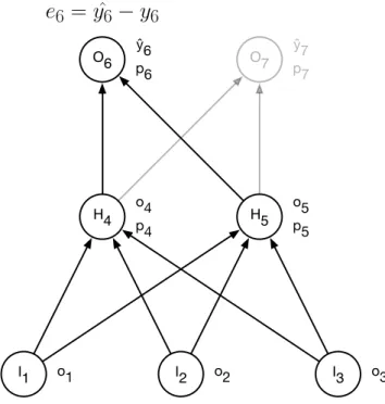
Being presented with a sample from the training set, backpropagation first runs it through the network in order to get an actual output. The algorithm is supervised, meaning we already know the ideal output. By comparing actual and ideal output, we get the output error: ei = yˆi −yi, wherei is the output neuron index. As illustrated in figure 2.7a, this forward pass will necessarily also calculate pre-activations and activations throughout the network, denotedpiandoi respectively.

Once the output error is obtained, we can start propagating the error through the network in reverse, hence the name backpropagation. Intuitively, we calculate how much each node contributed to the error in the layer above it, and adjust the associated weights accordingly. Contribution towards error is measured by the steepness of the error gradient. It is calculated by finding the partial derivative of the error function, with respect to a weightwij:

∂E ∂wij

=oiδj (2.2)

where δj represents the delta of neuron j in a given layer, and oi is the activation of neuroniin the layer below.

With all the activations already calculated during the forward pass, what remain to solve equation (2.2) are the node deltas δ. As specified

in equation (2.3), node deltas are calculated differently depending on the neuron type:

δ_i =

(

−eifi0(pi), output neurons

O6 ŷ_p66 O7 ŷ_p77 I1 o1 I2 o2 I3 o3 o5 p5 H5 H4 o4_p4

e

₆

= ˆ

y

₆

−

y

₆

(a) A forward pass is done to calculate output error.

O6 ŷ_p66 O7 ŷ_p77 I1 o1 I2 o2 I3 o3 o5 p5 H5 H4 o4_p4

e

₆

= ˆ

y

₆

−

y

₆

δ

6

=

−

e

6

f

6′

(

p

6

)

δ

₄

= (

δ

₆

w

_4,6

+

δ

₇

w

_4,7

)

f

₄′

(

p

₄

)

(b) Node deltas are propagated through the network in reverse.

where f_i is the neuron’s activation function and p_i is its pre-activation as defined by equation (2.1). An illustration is given in figure 2.7b.

The node deltas can now be used to calculate the error gradient for each neuron, following equation (2.2). All that remains is then to update the weights, based on the error gradients:

∆wij = η ∂E ∂wij

+α∆w0_ij (2.4)

whereηis thelearning rate,αthemomentumand∆w_ij0 represents the weight

delta from the previous iteration (set to zero for the first iteration). The learning rate hyper-parameter controls how much we let each training example influence the weight change. Momentum allows weights to change faster, given the change proceeds in the same direction through iterations.

Parallelization

As described here, backpropagation runs one iteration for every training sample, resulting in just as many weight updates. Learning can be greatly sped up by parallelizing, for example using a Graphics Processing Unit (GPU). In order to run iterations of backpropagation in parallel, weight updates naturally can not be performed after each training sample; that would require a sequential learning process. Instead, weight changes are accumulated and applied after every parallel iteration, each of which covers multiple training samples.

Limitations

For neural networks with multiple hidden layers, the algorithm introduces a problem calledvanishing gradients. Backpropagation uses the derivative of the activation function. Exemplifying with the logistic function, the gradient of extreme input come very close to zero. During the backpropagation, some weights will see small updates, due to vanishing gradients. As extreme activations are encountered further down the network, the effect is amplified to the point where weights barely change at all. The result is that top layers optimize normally, while lower layers require significantly more training.

Underfitting is not the only problem with deep architectures, as they are also prone to overfit. Multiple layers create expressive models where successive layers reason over increasingly higher-level, abstract features. Although this is a powerful property, it also means that these models have the complexity to fit fine details in the samples. As discussed in section 2.2.8, this will often lead to overfitting.

Dropout

By making a small change in the backpropagation algorithm, overfitting in deep architectures can be reduced. The technique is known asdropout,

and was introduced in [18]. During training, each hidden node is assigned a probability of being disabled, making it produce an activation value of zero. The decision whether to drop a node is made independently each time a node calculates its output, and the effect is necessarily only active until next activation.

Deactivating, or dropping neurons will hurt the performance of the network, since successive nodes can no longer rely on the preceding layer being complete. Furthermore, it is not predictable which nodes will be disabled. This means the hidden units have to be more general in their activations, potentially having to account for several disabled nodes. Experiments in [18] show a higher error rate with dropout for training set classification, but lower error rates for out-of-sample data. Note that dropout is strictly used for training.

Dropout adds one additional hyper-parameter, the probability of disabling a node. Possibly the optimal value of this parameter depends on the problem and data, but [18] points to 0.5 as a safe reference point.

Applications

Backpropagation is often exemplified using FFNNs, where each neuron in a layer is connected to all in the next. This is usually for pedagogical reasons, however the algorithm itself does not specifically require a fully connected architecture, as long as the network is directed and acyclic. Combined with great parallelizability for fast training, this makes backpropagation an effective and versatile learning algorithm for supervised learning.

2.3.4 Deep Learning

As discussed in section 2.3.3, training deep networks using backpropaga-tion presents some challenges. Deep learning is a popular term that refers to techniques that enables training deep architectures. Because deep net-works are prone to both underfitting and overfitting, deep learning algo-rithms address one or both of these issues. Unsupervised pre-training is discussed in section 2.5.3, and can be regarded as one of the breakthroughs in training deep models. The weight sharing found in Convolutional Neu-ral Networks (CNNs) reduce overfitting by forcing groups of neurons to use identical weights, see section 2.4.4. Dropout has already been men-tioned in section 2.3.3, and is another measure for reducing overfitting.

2.4

Supervised Models

The following section introduces models that use supervised learning to adjust their weights, as explained in section 2.2.2. These models require every training sample to be accompanied by an ideal output.

2.4.1 Recurrent Neural Network

While FFNNs only allow forwards connections, a Recurrent Neural Network (RNN) may contain feedback signals. This implies that RNNs keep updating an internal state known as context or memory, which in turn is considered when computing future states. Theoretically the temporal dependency may reach arbitrarily far back in time, although current learning algorithms and computational power enforce practical restrictions.

Introduced in [11], the Elman network is an early example of recurrent models. As depicted in figure 2.8, the model includes dedicated context units, marked C. Input, hidden, bias and output neurons are also shown. Each hidden unit outputs to its own context unit upon activation, making the context layer act as an internal memory. The context feeds delayed values back into the hidden layer, enabling the network to detect features based on current input and past states. Note that activations going into the context are weighted by a fixed value of one, essentially copying them over. Similarly, context neurons use the identity activation function, which simply outputs the input: f(p) = p.

I I O H H B B C C

Figure 2.8: The recurrent architecture known as an Elman network. Care context units.

Backpropagation Through Time

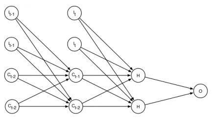
Elman networks, and RNNs in general, may learn by using a slightly modified version of backpropagation known as Backpropagation Through Time (BPTT). BPTT unfolds the network with respect to time, creating a deep, layered architecture (illustrated in figure 2.9). Because the feedbacks create a circular pattern, we cannot fully unfold the network. A hyper-parameter limits how far back the network should be traversed. Figure 2.9 unfolds two time steps.

The unfolded model can learn through normal backpropagation, with a couple of exceptions. Firstly, the input sequence is distributed over multiple layers, rather than the standard procedure of using the first layer

It-1 It-1 Ct-2 Ct-2 Ct-1 Ct-2 It It O H H

Figure 2.9: BPTT unfolds an RNN two steps through time, making it finite. Bias neurons are not shown.

as the only input layer. Secondly, the backwards pass will result in different weight adjustments for the same node at different unfolded layers. This can be dealt with by weight averaging. Note that the backpropagation issue of vanishing gradients mentioned in section 2.3.3 is especially relevant for BPTT, due to the circular structure of RNNs.

2.4.2 Echo State Network

Many attempts have been made to exploit recurrent architectures. A family of RNN models relies on using a fixed hiddenpoolorreservoirof neurons in order to simplify the learning procedure. Models like Echo State Networks (ESNs) [24] and Liquid State Machines (LSMs) [32] both fall under this category known asreservoir computing. As these two approaches are similar to each other, I choose to focus on the ESN due to its good results on the chaotic Mackey-Glass time series in the original paper [24]. LSM neurons are more biologically accurate, however this in itself is not a goal for this particular setting.

Using the same mathematical notation as in [24], figure 2.10 depicts an example ESN architecture: The input layeru, a sparsely (and typically randomly) connected reservoirxand an output layery. There are at most four sets of weights:Win for input to reservoir,W for internal connections and Wout for incoming output connections. Lastly the network may optionally incorporate output feedback connections, with corresponding weightsWback.

The next output layer state of an ESN is calculated as follows

y(n+1) = fout(Wout(u(n+1),x(n+1),y(n))) (2.5) where fout = (f₁out, ...,f_iout, ...,f_Lout), f_ioutis the activation function for output activation yi and (u(n+1),x(n+1),y(n)) is the concatenation between the respective activations. Note that the network can be configured not to

O I I I W Win Wout u H H H H H H H x y W

Figure 2.10: An ESN architecture. Illustration inspired by figure 1 in [24]. include connections from input to output and output to output. In doing so, equation (2.5) is simplified by eliminating the dependency onu(n+1)

andy(n).

Equation (2.5) depends on an updated internal state:

x(n+1) = f(Winu(n+1) +W x(n) +Wbacky(n)) (2.6) where f = (f1, ...,fi, ...,fN), fi is the activation function for internal activation xi. As mentioned the output-to-reservoir connections are optional, and architectures like figure 2.10 that do not use them may eliminate the expressionWback_{y(n)from equation (2.6).}

By fixing all but the output weights the learning problem is reduced to a linear regression problem. This is the key feature that makes ESNs efficient to train, but it also requires a reasonably weighted reservoir. There are several hyper-parameters that impact how the weights are initialized. As the name suggests,input scalingis an interval defining the upper and lower limit between which input weights are randomly sampled. Spectral radius of the reservoir can be adjusted to scale its weights. [31] points out that tasks with longer temporal dependencies usually require larger spectral radii. On the other hand, a large spectral radius might violate theecho state property, expressing that internal states should be uniquely defined by the input and its fading history, see [24, 31]. In other words, we want the input to echo around the network for a certain number of steps, but not indefinitely. Specifically, a spectral radius below one is likely to maintain the echo state property. Thereservoir capacitycontrols the number of internal neurons.

2.4.3 Time-Delay Neural Network

[51] considers the task of recognizing phonemes, the atomic sound units that make up speech. Extracting them from audio input is challenging for fully connected FFNNs, mainly because spoken sentences contain pauses

of variable length between words. If the model is presented with an unseen sample where the location and length of pauses are dissimilar to training samples, it is likely to produce ambiguous activations that arewashed outby pause noise. Traditionally, phoneme recognition therefore required heavy pre-processing of the audio input, in order to identify where individual phonemes begin and end.

Figure 2.11 shows a variation of the network architecture introduced in [51], intended for phoneme recognition. Time-Delay Neural Networks (TDNNs) use special neurons that have separate weights for differentdelays

of an input. How many time steps to delay, is domain-specific. In the original paper [51], each neuron in the first hidden layer connected to three different versions of the input variables through time. Figure 2.11 denotes the time stepst...t₋5 for variablesv0...v3. Every row in the hidden layer is associated with a contiguous segment of time steps. Each neuron within the same row is connected to the input neurons representing said time steps. t-5 t-4 t-3 t-2 t-1 t v0 v1 v2 v3

Input Hidden Output

Figure 2.11: A fully unfolded TDNN architecture. The illustration is inspired by figure 2 in [51].

Because each TDNN hidden unit covers full spatial states within its own time window, [51] suggests units within the same row share their weights. This ensures features are recognizable at all time window positions of the input. Ultimately this means that even if two recognizable features are separated by noise, some of the hidden neurons are likely to find them without washing them out with noise. Sharing weights also reduces the number of parameters considerably.

As illustrated by figure 2.11, TDNNs are easily viewed as a partially connected FFNN. Training a TDNN can then be done using backpropaga-tion, or other FFNN learning algorithms.

2.4.4 Convolutional Neural Network

Although an FFNN trained with backpropagation theoretically might han-dle complex problems given enough neurons, it often requires significant amounts of time and resources. This is especially true when modeling high-dimensional data such as the pixels in images; not only can images be large in terms of resolution, but color images additionally consist of separate val-ues for each color channel.

The first Convolutional Neural Network (CNN) appeared in [13]. It was developed with image recognition in mind, inspired by how biological brains process visual input by dividing the signals into smaller areas called

receptive fields [20]. Several flavors of the artificial CNN exists, many of which are based on [28].

In addition to fully connected feed forward layers, CNNs introduce convolutional and sub-sampling layers. Convolutional layersrepresent the artificial counterpart to biological receptive fields, whilesub-sampling layers

offer a simple, dynamic way of reducing the data dimensionality.

As shown in figure 2.12, CNN layers may be separated into several

feature maps: The first convolutional layer (marked C) consists of four feature maps, while the second has two feature maps. As the name suggests, each feature map represents the presence or absence of a particular feature in different parts, or receptive fields, of the input image. The input layer may also consist of several maps, as in the case for color images.

I C P C F O

Figure 2.12: A CNN architecture, inspired by figure 2 in [28]. C, P andF

are convolutional, pooling and fully connected layers, respectively.

Convolution

Convolutional layers exploit the spatial relationship between groups of pixels. For each neuron in a convolutional layer feature map, its activation represents the presence of a feature in the associated receptive field. Note that all neurons in a feature map respond to the same feature, but at different locations in the previous layer. This enables them to share the same set of weights, reducing the parameter count and allowing for

efficient learning.

Feature maps are constructed so that neighboring receptive fields are represented by neighboring feature neurons. This ensures that the spatial relationship between local pixels is preserved in the feature map. Because of this property we are able to stack convolutional layers on top of each other, creating deep networks.

Receptive fields may overlap, making it possible to isolate a feature from its environment. Imagine trying to classify a small tennis ball in a large picture; because we allow overlapping receptive fields, the chances of a neuron having its receptive field filled with the tennis ball increases, rather than four neurons containing 25% of a tennis ball.

Another property of convolutional neurons is that their receptive fields actually span across all feature maps within their input layer. This ensures that multiple features are considered when finding new ones. Such behavior resembles fully connected FFNNs.

Sub-sampling

Convolutional layers do not necessarily produce feature maps of signifi-cantly smaller size than the input maps. Furthermore, the number of fea-ture maps in a convolutional layer may be arbitrarily large, depending on how many features we wish to extract. To help deal with high-dimensional data and vast amounts of features, CNNs use sub-sampling or pooling in order to reduce dimensionality.

There are multiple ways of sub-sampling feature maps, and two common techniques are min-pooling and max-pooling. Similar to the receptive fields of convolutional neurons, a pooling neuron is associated with a spatial regionwithin the previous layer. Assuming max-pooling, pooling neurons activate with