Modified Shuffled Frog Leaping Algorithm based 6DOF Motion for Underwater Mobile Robot

(1)

Procedia Technology 10 ( 2013 ) 295 – 303

Selection and peer-review under responsibility of the University of Kalyani, Department of Computer Science & Engineering doi: 10.1016/j.protcy.2013.12.364

ScienceDirect

International Conference on Computational Intelligence: Modeling, Techniques and

Applications (CIMTA- 2013)

Modified Shuffled Frog Leaping Algorithm based 6DOF Motion

for Underwater Mobile Robot

Shubhasri Kundu

a,

a*, Dayal R. Parhi

a a

1.Introduction

Robotics Laboratory, Department of Mechanical Engineering, NIT Rourkela, Rourkela-769008, India

Abstract

Optimal path in an environment containing obstacles for underwater vehicle can be computed using a numerical solution of the nonlinear optimal control problem (NOCP). The underwater vehicle is modelled with six-dimensional nonlinear and coupled equations of motion, controlled by DC motors in all degrees of freedom. The intent of this computation is to offer a comprehensive perception of the behaviour of underwater autonomous vehicle and also to obtain the unknown parameters of the model which can be devoted in motion planning strategy of underwater robot. To execute tasks along a distinctive path in a convoluted environment, motion planning necessities to concede the underwater robot to be in motion between its current and final configurations without any collision within the encircling environment. Traditional optimization methods are not very effective to it, which are easy to plunge into local minimum. The optimization of path as well as time taken has been analysed here using modified shuffled frog leaping (SFL) optimization algorithm based on perception, cognition and sensor fusion. Path scheduling has to be executed for achieving integration of different preliminary robotic behaviours (e.g. obstacle avoidance, wall and edge following, escaping dead end and target seeking) in partially unknown territory (land or water). The optimal path is generated with this method when the robot reaches its target. The simulation studies ensure that the heuristic navigational approach possesses intelligent decision-making capabilities in negotiating hazardous terrain conditions during the under-water robot motion.

Selection and peer-review under responsibility of the University of Kalyani, Department of Computer Science & Engineering. Keywords : Optimal path; Obstacle avoidance; Target Seeking behaviour; memplex;

* Corresponding author. Tel.: +0-661-246-4509; fax: +0-661-246-2022. E-mail address: [email protected].

(2)

Path planning is a vital task necessary in the design of AUVs, which is to search out an optimal or sub-optimal path between an initial position and the desired target under specific constraint conditions [1]. Its goal is to plan a sequence of suitable paths subjected to some optimization criteria that allows the vehicle to complete its task objectives by reaching the specified destination point from the starting location without obstacle collision. To achieve this aim, researchers have propounded evolutionary algorithms (EAs) for searching near optimal solutions to problems [3]. EAs are stochastic search tactics that emulate the metaphor of natural biological evolution and the social behavior of species. A performance index, as a cost function that should be minimized, based on an approximation of the weighted combination of energy and time consumption is considered [4]. The time consumption can either be constrained or free. The use of time–energy-optimal paths can extend the period of operation for an autonomous battery powered underwater vehicle significantly. This type of vehicle can be used for underwater assessment and telerobotics.

A novel method of local path optimization based on the position of the target and the obstacles has been addressed. During the process of SFL [7, 13], the position of the globally best frog in each iterative is selected, and reached by the robot in sequence. We assume each obstacle as a point in centre of the obstacle and this information is known for our algorithm but the shape, size, and other geometries from the environment and obstacle are unknown and robot path planning processor updates the information on path [5, 6]. With this method the robot can automatically deal with the changes of the unknown environment and get some global optimization effect by using the information of target and obstacles at the same time.

This paper is coordinated as follows: Section 2 describes kinematic modeling based on 6 DOF motion equations. Section 3 presents the formulation of proposed algorithm in a generalized manner. Section 4 relates the proposed algorithm to the path planning problem which has been currently chosen for research work. Section 5 demonstrates simulation result along with different number of obstacles distributed in a cluttered manner. Section 6 concludes this paper and presents some future works.

2.Kinematic Modeling of 3d Motion

The kinematic model of the system is acquired by contemplating the nonholonomic constraints on the linear velocity. The nonholonomic restraints confine the velocity of the system to be zero in certain directions, but these boundaries do not compel the global movement of the system [1]. Such limits can arise when two surfaces roll against each other or in space-based systems where the total angular momentum of the system is conserved. For the analysis of motion of underwater robot in 6 DOF, it is necessary to work with two right-handed, orthogonal coordinate systems. To measure distances and angles, an earth-fixed reference frame has chosen as an inertial frame, denoted by {E} (o, XE, YE, ZE) and a reference frame is assumed to be fixed to a chosen point on the body, denoted

by {B} (b, XB, YB, ZB

2.1.Linear velocity transformation relative to earth reference frame ) (Fig. 1).

In this formulation, we will express the translational and rotational position and velocity of a vehicle-fixed coordinate frame {B} relative to an inertial coordinate frame {E}, using rotation matrixes. Euler reasoned that any rotation from one frame to another can be visualised as a sequence of three simple rotations from {E} to {B}. The order of rotations is according to convention.

XE b {B} {E} ZE YE YB ZB XB Ʌ ߶ \

(3)

Fig. 1. Body fixed and earth fixed coordinate systems

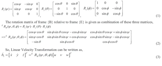
By the use of Euler angle representation [2], mathematically expression for three rotation matrices is as follows,

cos sin 0 ( ) sin cos 0 0 0 1 z R \ \ \ \ \ ª º « » « » « » ¬ ¼_, cos 0 sin ( ) 0 1 0 sin 0 cos y R T T T T T ª º « » « » « » ¬ ¼_, 1 0 0 ( ) 0 cos sin 0 sin cos x R I I I I I ª º « » « » « » ¬ ¼ ₍₁₎

The rotation matrix of frame {B} relative to frame {E} is given as combination of these three matrices, ( , , ) ( ) ( ) ( )

cos cos sin sin cos cos sin cos sin cos sin sin ( , , ) sin cos sin sin sin cos cos cos sin sin sin cos

sin sin cos cos cos

E B z y x E B R R R R R \ T I \ T I \ T I T \ I \ I T \ I \ \ T I \ T I T \ I \ I T \ I \ T I T I T ª º « » ! _« _» « » ¬ ¼₍₂₎

So, Linear Velocity Transformation can be written as,

>

@

>

@

1 ( , , )

T E T

B

b x y z R \ T I u v w ₍₃₎

2.2.Angular velocity transformation relative to earth reference frame

To derive angular velocity, the alignment of the body fixed reference frame with respect to the earth fixed reference frame can be depicted as:

>

@

0 0

0 ( ) ( ) ( ) 0

0 0

1 0 0 0 1 0 0 co s 0 sin 0

0 0 cos sin 0 cos sin 0 1 0 0

0 0 sin cos 0 0 sin cos sin 0 cos

T x x y p q r R R R I I T I T \ I T T I I T I I I I I I T T \ § · § · § · ¨ ¸ ¨ ¸ ¨ ¸ ¨ ¸ ¨ ¸ ¨ ¸ ¨ ¸ ¨ ¸ ¨ ¸ _{© ¹} _© _¹ © ¹ § · ª º § · ª º ª º § ¨ ¸« »¨ ¸« » « »¨ ¨ ¸ « »¨ ¸ « » « »¨ ¨ ¸ ¨ ¨ ¸ «_¬ »_{¼ © ¹ ¬}« » «_{¼ ¬} »_{¼ ©} © ¹ 2 sin 1 0 sin

cos sin cos 0 cos sin cos sin cos cos 0 sin cos cos

( , ). E B W b I T\ T I IT I T\ I I T T IT I T\ I I T \ I T · ¸ ¸ ¸ ¹ § · § ·§ · ¨ ¸ ¨ ¸¨ ¸ ¨ ¸ ¨ ¸¨ ¸ ¨ ¸ ¨ ¸ _© _¹¨ ¸ © ¹ © ¹ (4) As E

( , )

B

W

I T

is undefined or singular for pitch angle ofT r900_{, rotational transformation matrix does not} satisfy orthogonal property of matrices. Therefore, transpose ofE

( , )

B

W

I T

cannot be taken as inverse of the matrix.

>

@

1 2

1 sin tan cos tan

( , ) 0 cos sin

0 sin sec cos sec

T E B p b W p q r q r I T I T I T I I I T I T § ·§ · ¨ ¸¨ ¸ ¨ ¸¨ ¸ ¨ ¸¨ ¸ © ¹© ¹ (5) 2.3.6DOF Motion Equation

(4)

Summarizing the linear and angular velocity transformation matrices, kinematic equation can generalized for 6 DOF motion of body fixed reference frame {B} with respect to earth fixed reference frame {E} in a reduced form:

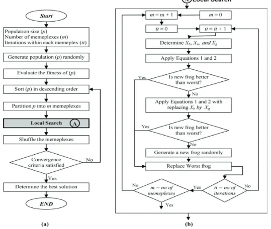
3 3 1 1 3 3 2 2 ( , , ) 0 0 ( , ) ( ) E B E B E B x u y v z R w b p W b q r P T b V \ T I I I T T \ u u § · § · ¨ ¸ ¨ ¸ ¨ ¸ ¨ ¸ ¨ ¸ ¨ ¸ § · § · ¨ ¸ ¨ ¸ ¨ ¸ ¨ ¸ © ¹ ¨ ¸ ¨ ¸ © ¹ ¨ ¸ ¨ ¸ ¨ ¸ ¨ ¸ ¨ ¸ ¨ ¸ © ¹ © ¹ ! (6) 3.Formulation of Shuffled Frog Leaping Algorithm

The shuffled frog-leaping algorithm is a memetic metaheuristic that is designed to seek a global optimal solution by performing a heuristic search. The SFL algorithm mingles the advantages of the genetic-based memetic algorithms and the social behavior based PSO algorithms [9]. Let us consider a group of frogs leaping in a swamp. The swamp has a number of stones at discrete locations where the frogs can leap onto. The goal of all the frogs is to find the stone with the maximum amount of available food as quickly as possible through improving their memes. The frogs can communicate with each other, and can improve their memes by passing information on each other. Improvement of the memes results in changing an individual frog’s position by adjusting its leaping direction and step size. A shuffling scheme permits for the swap of information between local searches to proceed toward a global optimum [10]. The SFL algorithm is described by flowchart in Fig. 2.

In the SFL, the population is partitioned into subsets referred to as memeplexes. The distinct memeplexes are deemed as dissimilar cultures of frogs, each enacting a local search. Within each memeplex, the discrete frogs grasp ideas, which can be motivated by the ideas of other frogs, and evolve through a process of memetic evolution. After a specified number of memetic evolution steps, concepts are passed among memeplexes in a shuffling process [8]. The local search and the shuffling processes endure until stated convergence criteria are assured [11]. The SFL algorithm can be described as below:

3.1.Global Search Step 0: Initialize

m: number of memeplexes ;

n : number of frogs in each memeplex; Total sample size, F = mn

Step 1: Generate a virtual population

Virtual Frog Population {U(1), U(2),……….., U(F)}; ith frog can be represented as, ;

Where d is the decision variables (i.e. number of memotype(s) in a meme carried by a frog). Compute the fitness value f (i) for each frog U(i) by using Triangular Probability function. Step 2: Rank frogs

Sort the F frogs in order of decreasing performance value. Store them in an array X = {U(i), f (i); i = 1, . . . , F }; Record the best frog’s position, as PX

Partition array X into m memeplexes each containing n frogs such as, Where, j=1,…..n; k=1,……m

Step 4: Memetic evolution within each memeplex

Evolve each memeplex according to the Local Search procedure of SFLA = U(1)

Step 3: Partition frogs into memeplexes

1 2 ( ) { , ,..., d} i i i U i U U U [ ( ) , ( ) | ( ) ( ( 1), ( ) ( ( 1))] k k k k k Y U j f j U j U k m j f j f k m j

(5)

Step 5: Shuffle memeplexes

After a defined number of memetic evolutionary steps within each memeplex, replace all memplexes into X, such that

_X

{ ,...,

_Y

1

_Y

m

}

; Sort X in order of decreasing fitness value; Update the population best frog’s position PX

3.2.Local Search

. Step 6: Check convergence

If the convergence criteria (Prespecified number of consecutive time loops) are satisfied, stop. Otherwise, return to step 3.

Evolution of each memeplex continues independently N times. After the memeplexes have been evolved, the algorithm returns to the global exploration for shuffling.

Step 0:

Set im = 0 ; where, im counts the number of memeplexes Set iN = 0; where iN counts the number of evolutionary steps Step 1:

Set im = im + 1 Step 2:

Set iN=iN+1

Step 3: Construct a submemeplex

Weights are assigned with a triangular probability distribution, ; where, j=1,….,n

Here, q distinct frogs are selected randomly from n frogs of each memeplex.

The submemeplex is sorted in descending order of performance, such as best (iq = 1) frog’s position PB and

worst (iq = q) frog’s position P Step size,

; for a positive step

W

Step 4: Improve the worst frog’s position

; for a negative step Where, rand() : Random number in range [0,1];

Smax

The new position is then computed by,

Compute the new performance value f(q). If the new f(q) is better than the old f(q) (i.e., if the evolution produces a benefit), then replace the old U(q) with the new one and go to step7. Otherwise go to step 5.

Step 5:

: Maximum step size allowed to be adopted by a frog after being infected

When step 4 cannot yield a better result, then Step and new position are computed for that frog by Step size, ; for a positive step

; for a negative step Again new position is then computed by,

Compute the new fitness value f(q). Step 6: Censorship

If the new position is either infeasible or not better than old position, the spread of defective meme is stopped by randomly generating a new frog r at a feasible location to replace the frog whose new position was not favourable to progress.

Compute f (r) and set U(q) = r and f(q) = f (r) Step 7: Upgrade the memeplex

After the memetic change for the worst frog in the submemeplex, replace array of submemplexes in their original locations.

Step 8:

After the memetic change for the worst frog in the submemeplex, replace array of submemplexes in their original

2 (1 ) / ( 1) j p n j n n max min{int[ ( _B _W)], } S rand P P S max max{int[rand P( BPW)],S } ( )q W U P S max min{int[ ( _X _W)], } S rand P P S max max{int[rand P( X PW)],S } ( )q W U P S

(6)

locations.

If iN < N, go to step 2. If im < m, go to step 1.

Otherwise return to the global search to shuffle memeplexes. A new solution can be randomly generated to replace that frog if no amendment is there.

Fig. 2. Flowchart of the shuffled frog-leaping algorithm 4. Modified SFLA as Path Planning Method

The problem considered in this section is underwater robot path planning in a partially unknown environment with static obstacles. During path planning, the real-time information is attained by the underwater robot sensors. The procedure of real-time path planning is divided into the following three steps. Firstly the path planning problem has been transformed into an optimization one, and also defined the optimization objective based on the target and the obstacles in the environment. The position of the globally best frog in each iterative is selected, and the underwater robot reaches these positions in sequence. The underwater robot constantly updates the information detected by its sensors, and the optimization objective function changes accordingly [7].

As is described in the above optimization process, each position to be reached by the underwater robot is evaluated based on the distance between itself and the target and obstacles in the environment [12]. Therefore the nearer a position to the target, the greater the fitness of the position should be; on the contrary, the nearer a position to the obstacles, the worse the fitness of the position should be.

Based on the above statement we denote T as the target, whose coordinate is (xT, yT , zT) . In addition, we

suppose that there are N obstacles in the environment, and denote them O = {O1,O2,……,ON}, we suppose them

as a point and their center coordinates are (xo1, yo1, zo1), (xo2 , yo2, zo2) ,……, (xoN, yoN, zoN) . It is possible for

(7)

robot to go there, so in each step the information is updated by the sensors and if there is a possibility of colliding, the direction of the movement will be changed by adjusting the speed of wheels. Afterward the fitness of a particle Piwhose coordinate is (xi, yi, zi

(9) Where ||.|| is a kind of norm.

) can be articulated as follows:

Here we take 2-norm, expressing the traditional distance between two points in 2 dimensional. It can be seen from (9) that when Pi is close to the target, the value of || Pi í7 __ ZLOO EH VPDOO $QG ZKHQ 3i

It can be got by analyzing (9) that when a frog comes close to the target, its fitness will decrease, resulting in it leaping toward the positions which are near the target. Selecting the position achieved by the globally best frog as the ones to be reached by the underwater robot in sequence, the path is to be formed with shorter length. So the path will have the length optimization by utilizing the information of the target. On the other hand when a frog is close to obstacles, the value will be small, resulting in a great fitness.

Therefore the frog has little opportunity to leap the positions near the obstacles. In addition, the positions of these obstacles are the maxima of (9), therefore are not reachable. That is to say, it is impossible for the underwater robot to collide with obstacles in the environment. It can be understood from (9) that w

is far from the obstacles the value o will be great. Therefore the problem solved by the SFL is a minimization one.

1and w2have influence on the

underwater robot’s path. When w1is great, the underwater robot will be far away from the obstacles, otherwise it

will be possible for the underwater robot to collide with them. When w2

5. Simulation Results

is great, the underwater robot has a strong trend to go to the target, resulting in the path being short; otherwise the path will be long. When the globally best position that was produced by the SFL algorithm, then we have to find out azimuth and elevation steering angle towards the selected position from the current position of the underwater robot.

To expound the effectiveness and the robustness of the proposed method in 3D underwater environment, simulation results on mobile robot navigation in various environments are exhibited. The obstacle avoidance behavior is activated when the readings from any sensors are less than the minimum threshold values (50mm). In the SFL algorithm, some assumptions are included such as: the number of frogs and the number of memeplexes are 60 and 6 respectively, maximum step size ze ze¨ XXXmax is set to 0.0125 and number of processing generations for each

memeplex before shuffling and number of shuffling iterations is 10 and 150 respectively. Also when the robot reaches near the target and the distance between the center of the robot and the target is less than 4cm the path planning process is stopped.

The result shows that the robot sets out from the start point, when it detects the obstacles in its path; the information of the obstacles is then transferred to the robot processor until the robot reaches the target. When an object is detected too close to the robot, it avoids a collision by moving away from it in the opposite direction.

Fig. 3. (a) Static obstacle avoidance behavior; (b) Navigational path traced by implementing SFLA based on Obstacle Avoidance and Target 1 ( ) min j i i 11 2. i i j OjO f P( )i) 11 w P T2. i P Oi j 1 1 1 1 w P22. i i value value j of oi j O O valu valu j P O_of_ofofofff j min j i j Oj O Pi Oj a a ((aa (a (a (a ( (a ( (a (a (a ( ( ( ( (a (a (a ( ( (a (a (a (a (a (a (aaaa (a (aaa (aaaaaaaa)a)))))))))))))))))))))))))))) (((((((b(((((((((bb)bbbbbbbbbbbbbbbb))))))))))))))) (((((((((((((cccc))))

(8)

Seeking behaviour; (c) Escaping from dead end obstacle by Wall Following behavior

Collision avoidance has the highest priority and therefore, it can override other behaviors, in this case, its main reactive behavior is avoidance of obstacles as shown in Fig. 3(a) and Fig. 3(b). Another special condition appears as the mobile robot detects an obstacle in the front while the target tracking control mode is on operation. In this case, the fixed wall following behavior should be performed first, the mobile robot must rotate clockwise or counterclockwise such that it can align and move along the wall (Fig. 3(c)).

We can see that with this method the robot gets the information and programs its path on-line in the partially unknown environment. In addition in proposed method the robot moves smoothly and reaches to its target by passing obstacles with a minimum distance.

The above figures reveal the path of the robot and the spots of the obstacles. The robot truly recognized obstacles and turned it and reached to the target, it can be seen that the robot reaches the target without colliding with the obstacles.

6.Conclusion

The major intents of this research work have been to find out efficient motion control techniques for underwater robot navigation in hazardous real world situations by avoiding collision with obstacles arranged in a chaotic way. In the path planning based on SFL algorithm, the position of globally best frog in each iterative is selected, and reached by the robot in sequence. The obstacles are detected by the robot sensors are applied to update the information of the environment. The optimal path is generated until the robot reaches its target. The simulation result validates the feasibility of the proposed method. It is noted that the path generated in each step is just feasible, that is to say, the robot can reach its target on condition of not colliding with obstacles. Although the programmed path has some optimal effect by using the information of the target and obstacles simultaneously, but we cannot guarantee that the obtained path is globally optimal. Also the simulation results show the effectiveness and robustness of this new algorithm and the robot moves smoothly toward its target. In near future more simulations as well as corresponding experimental verification will be carried out for validation of proposed technique. Comparison in performance by other navigation algorithms will also be in focus.

References

1. Fossen, T. I. (2002). Marine Control Systems: Guidance, Navigation and Control of Ships, Rigs and Underwater Vehicles. Marine Cybernetics. Trondheim, Norway.

2. Fossen, T. I. and J. P. Strand (2001). Nonlinear Passive Weather Optimal Positioning Control (WOPC) System for Ships and Rigs: Experimental Results. Automatica 37(5), 701—715.

3. Y. Hu and S. X. Yang, “A knowledge based genetic a1gorithm for path Planning of a mobile robot”, in Proc. IEEE Int. Conf. Robotics & Automation, New Orleans, LA, April 2004.

4. L. Lei, H. Wang and Q. Wu, “Improved genetic algorithms based path planning of mobile robot under dynamic and unknown environment”, in Proc. IEEE Int. Conf. Mechatronics and Automation, June 25 – 28, 2006, Luoyang, China.

5. C. Xin, Y.M. Li, “Smooth path Planning of a mobile robot using stochastic particle swarm optimization”, in Proc. IEEE. Int. Conf. Mechatronics and Automation Luoyang, China, 2006, pp. 1722– 1727.

6. I. Hassanzadeh, K. Madani, and M. A. Badamchizadeh, “Mobile Robot Path Planning Based on Shuffled Frog Leaping Optimization Algorithm”, 6th annual IEEE Conference on Automation Science and Engineering Marriott Eaton Centre Hotel Toronto, Ontario, Canada, August 21-24, 2010, pp:680-685.

7. Emad Elbeltagiy, Tarek Hegazyz and Donald Griersonz, “A modified shuffled frog-leaping optimization algorithm: applications to project management”, Structure and Infrastructure Engineering, Vol. 3, No. 1, March 2007, 53 – 60.

8. S. Y. Liong and M. D Atiquzzaman, “Optimal design of water distribution network using shuffled complex evolution,” J. Inst Eng., vol.44, Singapore, 2004, pp. 93–107.

9. M. M. Eusuff and K.E. Lansey, “Optimization of water distribution network design using the shuffled frog leaping algorithm,” Journal of Water Resources Planning and Management., vol. 129(3), 2003, pp. 210–225.

10. E. Elbeltagi, T. Hegazy and D. Grierson, “Comparison among five evolutionary-based optimization algorithms,” Advanced Engineering Information, vol. 19, 2005, pp 43-53.

11. Mohammad Rasoul Narimani, “A New Modified Shuffle Frog Leaping Algorithm for Non-Smooth Economic Dispatch”, World Applied Sciences Journal 12 (6): 803-814, 2011.

12. Mohammad Pourmahmood Aghababa, “3D path planning for underwater vehicles using five evolutionary optimization algorithms avoiding static and energetic obstacles”, Applied Ocean Research 38 (2012) 48–62.

(9)

13. E. Afzalan, M. A. Taghikhani and M. Sedighizadeh, “ Optimal Placement and Sizing of DG in Radial Distribution Networks Using SFLA”, International Journal of Energy Engineering 2012, 2(3): 73-77.