Adaptive Neuro Fuzzy Inference System (ANFIS) for Generation of Joint Angle Trajectory

(1)

AIJSTPME (2013) 6(2): 25-32

25

Adaptive Neuro Fuzzy Inference System (ANFIS) for Generation of Joint Angle

Trajectory

Nikhade G. R.

Department of Mechanical Engineering,Shri Ramdeobaba College of Engineering and Management, Nagpur-440013, Maharashtra (India)

Chiddarwar S. S.

Department of Mechanical Engineering, Visvesvaraya National Institute of Technology, Nagpur-440013, Maharashtra (India)

Deshpande V. S.

Department of Industrial Engineering,Shri Ramdeobaba College of Engineering and Management, Nagpur-440013, Maharashtra (India)

Abstract

In this paper, Adaptive Neuro-Fuzzy Inference System is utilized to learn from training data and create ANFIS with limited mathematical representation of the system. The proposed system consists of three phases i.e. Generation of training data, Execution of ANFIS, Generation of joint angle trajectory. The schematic of the proposed system is shown in Figure 4. The predicted joint angle configurations are further to be used to determine the trajectory for the task execution of the robot. The simulation studies conducted on a 5-DOF SCORBOT ER-IV robot manipulator shows the effectiveness of the approach over conventional techniques. Keywords: ANFIS, Robot, Trajectory, SCORBOT ER-IV

1 Introduction

A robot manipulator is composed of a serial chain of rigid links connected to each other by revolute or prismatic joints to perform a task in the 3-D space. A revolute joint rotates about a motion axis and a prismatic joint slides along a motion axis. Each joint location is usually defined relative to neighboring joints. The relation between successive joints is described by 4X4 homogeneous transformation matrices that contain orientation and position data of the robot [1]. The product of these transformation matrices produces final orientation and position data of a n-degree of freedom robot manipulator.

A robot manipulator is designed to perform a task in the 3-D space. The tool or end-effector is required to follow a planned trajectory to manipulate objects or carry out the task in the workspace. This requires control of position of each link and joint of the manipulator to control both the position and orientation of the end-effector. To program the tool motion and joint-link motions, a mathematical model

of the manipulator is required to refer to all geometrical and/or time-based properties of motion. A kinematic model describes the spatial position of the joints and links, and position and orientation of the end-effector.

In designing a robot manipulator, kinematics and dynamics play a vital role. The kinematic model gives relations between the position and orientation of the end-effector and spatial positions of joint links. Basically the kinematic modeling is split into two problems as forward kinematics and inverse kinematics. The forward kinematics problem is to determine the position and orientation of the end-effector from the given values of joint variables of the robot. The inverse kinematics problem is concerned with determining values for the joint variables that achieve a desired position and orientation for the end effector of the robot.

In practice, a robot manipulator control requires knowledge of the end-effector position and

(2)

Nikhade G. R. et al. / AIJSTPME (2013) 6(2): 25-32 orientation for the instantaneous location of each

joint as well as knowledge of the joint displacement required to place the end-effector in a new location. Therefore, direct and inverse kinematics are the fundamental problems of utmost importance of the robot manipulator’s position control. Many industrial applications such as welding and certain type of assembly operations require that a specific path should be negotiated by the end-effector. To achieve this, inverse kinematics are necessary to find the corresponding motion of each joint, which will produce the desired tool-tip motion.

2 Inverse kinematics

Inverse kinematics computations for a serial robot are elemental for design, analysis of workspace for path planning, trajectory planning and control, and offline programming of robots. Given the geometry of a robot and pose of its end-effector i.e. Cartesian position and orientation, the inverse kinematics (IK) computes all joint angle values for realizing that particular pose.

A serial robot consists of serial links connected in series by either revolute or prismatic or both types of joints. The kinematic control of such a serial robot involves the coordination of links of a kinematic chain to produce the desired motion. The path planners working in the background or in offline mode determine the Cartesian path for the robot and often devise the strategy for kinematic control of the robot. The execution of this Cartesian path demands for the conversion of Cartesian coordinates into joint angle coordinates. This conversion is done by the mapping Cartesian space of the robot into its joint space by using inverse kinematics relations. This mapping process is nonlinear due to the association of nonlinear trigonometric equations and becomes more complex for robots with complex geometry and multi-degree of freedom. Moreover, the associated problems like coupled nature of position and orientation kinematics of the robot, existence of multiple solutions and the presence of singularities add to the computational complexities.

The computation of inverse kinematics solutions for the control of a robot is attempted by means of various methods such as algebraic methods, geometric methods, numerical methods and neural network based methods. Algebraic and geometric methods are desirable because they are faster and easily identify all possible solutions, but algebraic methods do not guarantee closed form solution. For

the geometric method, closed form solutions for the first three joints of the manipulator must exist geometrically. The iterative methods converge to only a single solution depending on the starting point and will not work near singularities. The IK solution by these traditional methods is time consuming because of high complexity of the mathematical formulation if the joints of the manipulator are more complex [2]. Hence, a few attempts were made to apply artificial neural networks (ANN) for prediction of IK solutions for any particular robot. Essentially, ANN approximates inverse kinematics relations of a robot in order to map the Cartesian configuration into corresponding joint angles. The accuracy of predicted joint angles depends upon the method used for training of the network. Among the various methods used for training the network, back propagation neural network (BPANN), perceptron neural network and radial basis function (RBF) are the most commonly used methods. Out of them, BPANN is most popularly implemented to determine IK solutions of planar as well as articulated robots [3-6]. Certain hybrid techniques made use of ANN along with expert systems, fuzzy logic and genetic algorithm for obtaining IK solutions [7-9]. An IK solution of a two DOF planar robot was determined with an expert system that has made use of a modular neural network architecture [7]. An adaptive fuzzy logic approach was employed to determine IK solutions of a three DOF planar robot [8]. A neuro-genetic approach that combined ANN and a neuro-genetic algorithm was used to solve the IK problem of a two DOF planar robot [9]. These approaches can easily provide IK solutions for two or three DOF planar robots. On the contrary, these methods demand high performance computing systems and complex computer programming for obtaining the solutions of more DOF robots. In view of this, neural network based approaches are likely to be superior to hybrid methods. Among the existing networks, BPANN as well as perceptron neural network are time intensive due to the requirements of a higher number of epochs (iterations) for training of the network [8].On the contrary, an RBF neural network shows a faster convergence rate and high accuracy due to its ability of local approximation [10]. RBF along with a lookup table was used for predicting joint angles for two and three DOF planar robots [4]. Due to its faster convergence rate, it was also used for training the ANN for successful prediction of singularity free IK solutions of a six axis redundant robot [11]. Moreover, RBF can handle a large database very

(3)

Nikhade G. R. et al. / AIJSTPME (2013) 6(2): 25-32

27 effectively and converges quickly which makes it efficient to predict IK solutions within a short period.

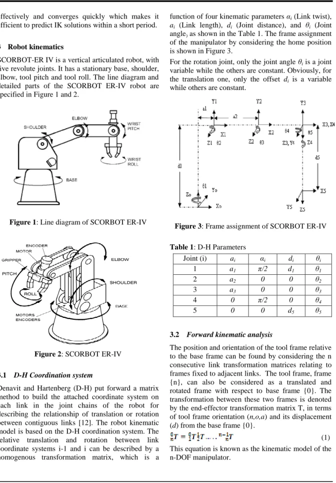
3 Robot kinematics

SCORBOT-ER IV is a vertical articulated robot, with five revolute joints. It has a stationary base, shoulder, elbow, tool pitch and tool roll. The line diagram and detailed parts of the SCORBOT ER-IV robot are specified in Figure 1 and 2.

Figure 1: Line diagram of SCORBOT ER-IV

Figure 2: SCORBOT ER-IV

3.1 D-H Coordination system

Denavit and Hartenberg (D-H) put forward a matrix method to build the attached coordinate system on each link in the joint chains of the robot for describing the relationship of translation or rotation between contiguous links [12]. The robot kinematic model is based on the D-H coordination system. The relative translation and rotation between link coordinate systems i-1 and i can be described by a homogenous transformation matrix, which is a

function of four kinematic parameters αi (Link twist),

ai (Link length), di (Joint distance), and θi (Joint

angle) as shown in the Table 1. The frame assignment of the manipulator by considering the home position is shown in Figure 3.

For the rotation joint, only the joint angle θi is a joint

variable while the others are constant. Obviously, for the translation one, only the offset di is a variable

while others are constant.

Figure 3: Frame assignment of SCORBOT ER-IV

Table 1: D-H Parameters Joint (i) ai αi di θi 1 a1 π/2 d1 θ1 2 a2 0 0 θ2 3 a3 0 0 θ3 4 0 π/2 0 θ4 5 0 0 d5 θ5

3.2 Forward kinematic analysis

The position and orientation of the tool frame relative to the base frame can be found by considering the n consecutive link transformation matrices relating to frames fixed to adjacent links. The tool frame, frame {n}, can also be considered as a translated and rotated frame with respect to base frame {0}. The transformation between these two frames is denoted by the end-effector transformation matrix T, in terms of tool frame orientation (n,o,a) and its displacement (d) from the base frame {0}.

(1) This equation is known as the kinematic model of the n-DOF manipulator.

(4)

Nikhade G. R. et al. / AIJSTPME (2013) 6(2): 25-32 To find the transformation matrix relating to two

frames attached to adjacent links, consider frame {i-1} and frame {i}. The transformation of frame {i-{i-1} to frame {i} consists of four basic transformations. 1. A rotation about zi-1axis by an angle θi

2. Translations along zi-1 axis by distance di

3. Translation by distance ai along xi axis and

4. Rotation by an angle αi about xi axis

Using the spatial coordinate transformation, the composite transformation, which describes frame {i} with respect to frame {i-1}, is obtained using equation (3). (2) for i= 1,2….n (3) where, Si = Sin(θi) Ci = Cos(θi) Cαi = Cos(αi) Sαi = Sin(αi) 3.3 Inverse kinematic analysis Opposite to the forward kinematic analysis, the corresponding variables of each joint could be figured out with the given location requirement of the end of the manipulator in the given reference coordinate system. This is called the inverse kinematic analysis, or kinematic inverse solution, multiplying each inverse matrix of matrices on the left side of above equation and then equalizing the corresponding elements of the equal matrices of both ends [13]. The desired location of the manipulator can be determined by equation (4). (4)

where, d is the translation of end effector from the reference frame. n, o, a describes the orientation of end-effector and represents the x, y, z axes of the end-effector After equating (Transformation matrix for the manipulator) to the end-effector tool point transformation matrix, the unknown joint angles can be determined: (5) (6) (7) (8) (9) (10)

4 Proposed ANFIS based approach

Figure 4: Schematic of the proposed ANFIS based

(5)

29 Figure 4 shows the architecture of the proposed ANIFS based system. The proposed system consists of three phases, 1. Generation of training data 2. Execution of ANFIS 3. Generation of joint angle trajectory. The working principle of each of these phases is given in the following section.

4.1 Generation of training data

ANFIS is the blend of a neural network and fuzzy inference system. Using a given input/output data set, the ANFIS constructs a fuzzy inference system (FIS) whose membership function parameters are adjusted using either a back propagation algorithm alone or in combination with a least squares type of method. This adjustment allows fuzzy systems to learn from the data used for modeling. Therefore, the data used for training this system plays an important role in demonstrating the effectiveness of the system. The joint space of the robot can be considered as an inverse image of the Cartesian space and vice versa. Similarly, the forward kinematics can be assumed to be an inverse image of inverse kinematics and vice versa. Based on this, it is decided to employ forward kinematics relations for determining the pose of the end-effector, i.e. P={X, Y, Z, Roll, Pitch, Yaw} corresponding to Q={1, 2, 3, 4, 5}. Hence, the pose P can be used as an input and the corresponding joint angle Q as the output for the ANFIS training data. In other words, a Q-P relationship is used while generating the data whereas P-Q mapping is done while training the ANFIS. ANN trained with such a data set is found to predict IK solutions more accurately due to insignificant mapping errors between input and output data [13] Hence, the same concept was also used for the ANFIS system. In this work, a total 5190 data sets were used for the training purpose.

4.2 Execution of ANFIS

ANFIS has a network-type structure similar to that of a neural network. It maps inputs through input membership functions and associated parameters, and then outputs through output membership functions and associated parameters to outputs. The parameters

associated with the membership functions change through the learning process. The computation of these parameters (or their adjustment) is facilitated by a gradient vector. This gradient vector provides a measure of how well the fuzzy inference system is modeling the input/output data for a given set of parameters. When the gradient vector is obtained, any of several optimization routines can be applied in order to adjust the parameters to reduce some error measure. This error measure is usually defined by the sum of the squared differences between actual and desired outputs. ANFIS uses either back propagation or a combination of least squares estimation and back propagation for membership function parameter estimation. In this work, genfis3 function of FUZZY Toolbox of Matlab was used to generate a FIS using fuzzy c-means (FCM) clustering by extracting a set of rules that models the data behavior. The function requires separate sets of input and output data as input arguments. The rule extraction method first uses the fcm function to determine the number of rules and membership functions for the antecedents and consequents. The number of clusters determines the number of rules and membership functions in the generated FIS. For this work, the number of clusters was selected automatically by the command. The input membership function was selected to be 'gaussmf', and the output membership function was selected to be 'linear'. The input and output was given to genfis3 using the database generated in the first phase of the approach. The number of iterations for genfis3 was selected to be 1000 and the tolerance to be 0.001 after certain trials. In this way, the training process of ANFIS was executed.

4.3 Testing and validation of ANFIS

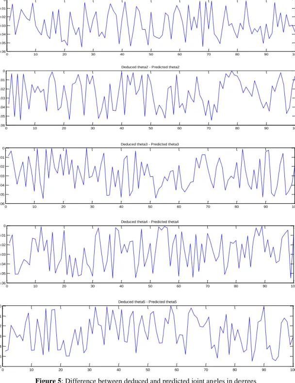
After executing the ANFIS based programme, in order to check the validity and accuracy of obtained results testing and validation was done by comparing the joint angle predicted by ANFIS and obtained using inverse kinematic equations. For this purpose, a set of 1000 configurations was selected randomly from the training data set of 5190. The difference between predicted and calculated joint angles is displayed in Figure 5.

(6)

Nikhade G. R. et al. / AIJSTPME (2013) 6(2): 25-32 0 10 20 30 40 50 60 70 80 90 100 -0.06 -0.05 -0.04 -0.03 -0.02 -0.01 0 TH E TA 1D TH E TA 1P

Deduced theta1 - Predicted theta1

0 10 20 30 40 50 60 70 80 90 100 -0.06 -0.05 -0.04 -0.03 -0.02 -0.01 0 TH E TA 2 D TH E TA 2 P

0 10 20 30 40 50 60 70 80 90 100 -0.06 -0.05 -0.04 -0.03 -0.02 -0.01 0 TH E TA 3 D TH E TA 3 P

0 10 20 30 40 50 60 70 80 90 100 -0.06 -0.05 -0.04 -0.03 -0.02 -0.01 0 TH E TA 4 D TH E TA 4 P

0 10 20 30 40 50 60 70 80 90 100 -0.06 -0.05 -0.04 -0.03 -0.02 -0.01 0 TH E TA 5 D TH E TA 5 P

Figure 5: Difference between deduced and predicted joint angles in degrees

The graphs shown in Figure 5 represent the error between the values of joint angles predicted by ANFIS and calculated from the inverse kinematic equations. The average error in prediction of all joint angles using ANFIS is around ±0.04 degree. This

error is very small as compared to the minimum joint angle increment possible with all five joints of the robot. This shows that the ANFIS used for training and inference purpose works very well. In order to test, the applicability of the proposed ANFIS based

(7)

31 approach, a sample Cartesian trajectory is decided for the SCORBOT and the corresponding joint angle trajectory is determined in the next section.

5 Generation of trajectory

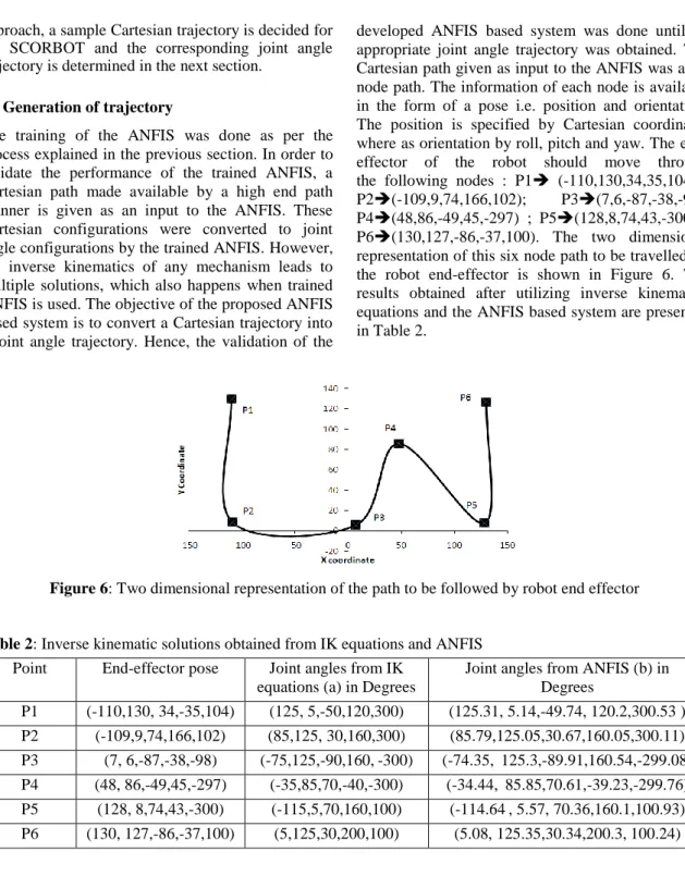
The training of the ANFIS was done as per the process explained in the previous section. In order to validate the performance of the trained ANFIS, a Cartesian path made available by a high end path planner is given as an input to the ANFIS. These Cartesian configurations were converted to joint angle configurations by the trained ANFIS. However, the inverse kinematics of any mechanism leads to multiple solutions, which also happens when trained ANFIS is used. The objective of the proposed ANFIS based system is to convert a Cartesian trajectory into a joint angle trajectory. Hence, the validation of the

developed ANFIS based system was done until an appropriate joint angle trajectory was obtained. The Cartesian path given as input to the ANFIS was a six node path. The information of each node is available in the form of a pose i.e. position and orientation. The position is specified by Cartesian coordinates where as orientation by roll, pitch and yaw. The end-effector of the robot should move through the following nodes : P1 (-110,130,34,35,104) ; P2(-109,9,74,166,102); P3(7,6,-87,-38,-98); P4(48,86,-49,45,-297) ; P5(128,8,74,43,-300) ; P6(130,127,-86,-37,100). The two dimensional representation of this six node path to be travelled by the robot end-effector is shown in Figure 6. The results obtained after utilizing inverse kinematics equations and the ANFIS based system are presented in Table 2.

Figure 6: Two dimensional representation of the path to be followed by robot end effector

Table 2: Inverse kinematic solutions obtained from IK equations and ANFIS

Point End-effector pose Joint angles from IK equations (a) in Degrees

Joint angles from ANFIS (b) in Degrees P1 (-110,130, 34,-35,104) (125, 5,-50,120,300) (125.31, 5.14,-49.74, 120.2,300.53 ) P2 (-109,9,74,166,102) (85,125, 30,160,300) (85.79,125.05,30.67,160.05,300.11) P3 (7, 6,-87,-38,-98) (-75,125,-90,160, -300) (-74.35, 125.3,-89.91,160.54,-299.08) P4 (48, 86,-49,45,-297) (-35,85,70,-40,-300) (-34.44, 85.85,70.61,-39.23,-299.76) P5 (128, 8,74,43,-300) (-115,5,70,160,100) (-114.64 , 5.57, 70.36,160.1,100.93) P6 (130, 127,-86,-37,100) (5,125,30,200,100) (5.08, 125.35,30.34,200.3, 100.24)

From Table 2, it can be seen that the results obtained using IK equations and the ANFIS based approach are comparable. The difference between predicted joint angles and expected joint angles lies in the decimal places of the observed values. The graphs shown in Figure 6 and the results shown in Table 1

are little different. The main reason is that the ANFIS based algorithm was used for a greater number of observations whereas the configurations used in the example are less. However, the results are comparable.

(8)

6 Conclusions

This paper has compared the IK solutions obtained from the IK equations for a SCORBOT ER-IV and ANFIS based approach. The idea of using forward kinematics equations for generating training data for ANFIS led to a nearly accurate training of the ANFIS network. The proposed approach shows advantages over IK equations because the latter needs to utilize complex concepts of mathematics and trigonometry. Moreover, ANFIS based systems need more data for improved performance. Hence, considerable more time is required for training, testing and validation. Another problem associated with ANFIS is handling two inputs and one output at a time. This leads to utilization of multiple ANFIS networks especially when one is dealing with a higher degrees of freedom robot. Despite of these shortcomings, the proposed ANFIS based approach is very useful for obtaining inverse kinematic solutions as it can work as a control algorithm. The authors are planning to use this approach for the generation of a robot trajectory for welding operations in the future.

References

[1] Srinivasan Alavandar, M.J. Nigam, 2008. Inverse Kinematics Solution of 3DOF Planar Robot using ANFIS, Int. J. of Computers, Communications & Control, ISSN 1841-9836, E-ISSN 1841-9844, 3: 150-155.

[2] Raşit KÖKER, 2011. A Neuro-Genetic Approach to the Inverse Kinematics Solution of Robotic Manipulators, Scientific Research and Essays, 6(13): 2784-2794.

[3] Morris, A. S. and Mansor, A., 1997. Finding the Inverse Kinematics of Robot Arm using Artificial Neural Network with Lookup Table, Robotica, 15: 617-625.

[4] Morris, A. S. and Mansor, A., 1998. Robot Inverse Kinematics using an Adaptive Back Propagation Algorithm and Radial Basis Function with a Look Up Table, Robotica 16: 433-444.

[5] Hasan, A. T.et. al., 2006. An Adaptive Learning Algorithm To Solve The Inverse Kinematics Problem of A 6 DOF Serial Robot, Advances in Engineering Software, 37: 432-438.

[6] Lou, Y. F. and Brunn, P., 1999. A Hybrid Artificial Neural Network Inverse Kinematic Solution for Accurate Robot Path Control, Proceedings of the Institution of Mechanical Engineers, Part I: Journal of Systems and Control Engineering, 213(1): 23-32.

[7] Oyama, E., Agah, A., MacDorman, K.F., Maeda, T., Tachi S., 2001. A Modular Neural Architecture for Inverse Kinematics Model Learning, Neurocomputing, 38(40): 797- 805. [8] Baheshti, M. T. H., Tehrani, A. K., Ghanbari, B.,

2003. An Optimized Adaptive Fuzzy Inverse Kinematics Solution for Redundant Robots, Proceedings of International Symposium on Intelligent Control, Houston, Texas, 924-929. [9] Kalra, P. and Prakash, N. R., 2003. A Neuro

Genetic Algorithm Approach for solving Inverse Kinematics of Robotic Manipulators, Proceedings of the IEEE International Conference on Systems, Man and Cybernetics, Washington, DC, 2: 1979-1984.

[10] Zhang, P. Y., Lu, T.S. and Song, L.B., 2005. RBF Network based Inverse Kinematics of 6R Robot, International Journal of Advance Manufacturing Technology, 26: 144-147. [11] Mayorga, R. and Sanongboon, P., 2005. An

Artificial Neural Network Approach for Inverse Kinematics Computation and Singularities Prevention of Redundant Robots, Journal of Intelligent and Robot Systems, 44: 1-23. [12] Wen Guojun Xu Linhong He Fulun, 2009.

Offline Kinematics Simulation of 6-DOF Welding Robot, International Conference on Measuring Technology and Mechatronics Automation, 283-286.

[13] Mahdi Salman Alshamasin, 2009. Kinematic Modeling and Simulation of a SCARA Robot by using Solid Dynamics and Verification by MATLAB/Simulink, European Journal of Scientific Research ISSN 1450-216X, 37(3): 388-405.

[14] Chiddarwar, S. S. and Ramesh Babu, N., 2008. Inverse kinematics of 6R Serial Robot using Radial Basis Function based Approach, Proceedings of 2nd International and 23rd All India Manufacturing Technology, Design and Research Conference, IIT Madras, Chennai, Dec. 15-17, 2: 901-906.