Climate Change Impacts on Thermal Performance of Residential Buildings

(1)

Soroush Samareh Abolhassani

A Thesis in the Department

of

Building, Civil and Environmental Engineering

Presented in Partial Fulfilment of the Requirements

for the Degree of Master of Applied Science (Building Engineering) at Concordia University

Montreal, Quebec, Canada

July 2018

(2)

CONCORDIA UNIVERSITY School of Graduate studies This is to certify that the thesis prepared

By: Soroush Samareh Abolhassani

Entitled Climate Change Impacts on Thermal Performance of Residential Buildings

And submitted in partial fulfillment of the requirements for the degree of Master of Applied Science (Building Engineering)

Complies with the regulations of the University and meets the accepted standards with respect to originality and quality.

Signed by the final Examining Committee:

____________________________ Chair Dr. C. Mulligan ____________________________ Examiner Dr. L. Wang ____________________________ Examiner Dr. C. Mulligan ____________________________ Examiner Dr. C. El Ayoubi ____________________________ Supervisor Dr. F. Haghighat ____________________________ Supervisor Dr. A. Nazemi Approved by _____________________________________________________ Chair of Department or Graduate Program Director

July 2018 _____________________________________________________ Dean of Faculty

(3)

Abstract

Climate Change Impacts on Thermal Performance of Residential Buildings Soroush Samareh Abolhassani

Climate change has altered regular temperature patterns and various climate variables on a global scale, causing growing concerns about future food, water and energy security. Immediate action should be taken to understand the extent of climate change while also proposing adaptation strategies to cope with the projected future climate conditions. From the energy security perspective, particularly in consideration of the ever-increasing human population, an important aspect to understand is the impact of climate change on the energy consumption of residential buildings. Understanding the impact of climate change on building energy consumption is not only beneficial for advising efficient energy-saving measures, but also for understanding future energy requirements. Various studies have already shown that climate change effects heating and cooling loads of buildings in various climates around the world. However, there is a lack of comprehension of the effects of climate change on energy consumption in Quebec. In addition, some of the methodologies employed to address the impact of climate change in buildings may be not be accurate or accessible to practitioners. The present study tries to fill this gap by advising a simple procedure that can be implemented in day-to-day engineering practice for a detailed understanding of the effects of climate change on building energy consumption. The methodology is applied to a residential building in Montreal, Quebec (Canada), using the state-of-the-art climate model projections for the periods of 2011-2040 (short-term future), 2041-2070 (midterm future), and 2071-2100 (long-term future) and under low and high greenhouse gas concentration scenarios. In brief, the available projections of five global climate models was studied for two particular weather parameters, namely dry-bulb temperature and shortwave radiation. The projections were downscaled at the point location and at an hourly resolution using a cascade model based on a quantile mapping bias correction method and a modified quantile-based k-nearest neighbor method. The downscaled projections were used as inputs to TRNSYS, an energy simulation software, in order to quantify the heating and cooling loads as well as judge the overall performance of the residential building in Montreal. This methodology can provide a basis for

(4)

detailed understanding of the impacts of climate change on building energy consumption. Considering the applied case study, it is understood that climate change will not only change the intensity of the heating and cooling loads but can also change the empirical distribution of hourly energy consumption, particularly during peak loads.

(5)

Acknowledgments

I would like to express my deepest gratitude and respect to my supervisors, Professors Fariborz Haghighat and Ali Nazemi, who supported me throughout my research and study at Concordia University. They have devoted their time to assisting me throughout the duration of this project and they were always welcoming, even meeting with me out of the normal office hours. I am, and always will be, sincerely grateful for the opportunity they have given me in realizing this project, for their guidance, and their constant support. The freedom that they gave me and their trust in my abilities was truly rewarding for me

I also want to deeply thank my colleagues (Behrang, Emilie, Helene, Dave, Mahmood, Maryam, Jenny, Ying, Li, Karthik, and Mojtaba) for their kindness, their humour, their help and their patience with my English. This experience would have been completely different without the fun and relaxed atmosphere in our office.

Last, but not least, my sincere and heartfelt thanks go out to my mother, Azadeh Sohrabian, my father, Said Samareh Abolhassani, my grandfather, Mr. Mashallah Samareh Abolhassani, and my sister, Aysa Samareh Abolhassani.

(6)

List of Figures

Figure 1: Representative concentration pathways based on radiative forcing [2] ... 8

Figure 2. Different downscaling methods ... 10

Figure 3: The procedure of bias correction quantile mapping downscaling method [31] ... 15

Figure 4: Summary of results for Hong Kong, China ... 24

Figure 5: Photo of the experimental house [85]. ... 33

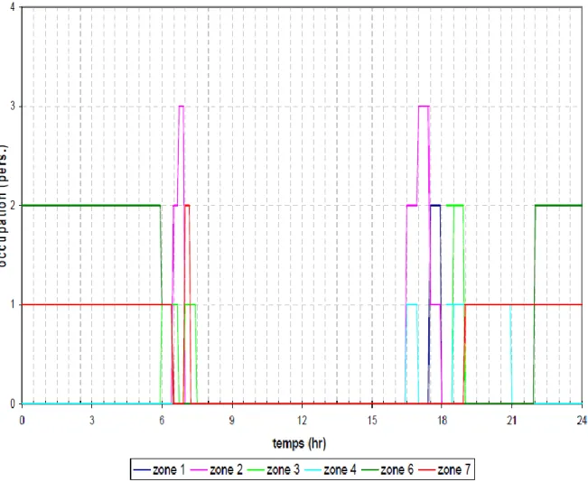
Figure 6: Weekly occupancy schedule on the ground floor ... 34

Figure 7: Framework for generating local future weather data ... 36

Figure 8: Framework for generating local future diffuse horizontal, and direct normal radiation ... 36

Figure 9: Methodology showing the bias correction (quantile mapping) downscaling process ... 41

Figure 10: Cumulative distribution function of GCM bias corrected, observation, and GCM historical data compared for three weather parameters; a) Daily dry bulb temperature, and b) Daily radiation ... 41

Figure 11: The procedure of disaggregation method for temporal downscaling ... 42

Figure 12: Methodology showing the temporal downscaling (disaggregation) process ... 44

Figure 13: Connection between the TMY file and type 16 mode 2 in TRNSYS model. ... 46

Figure 14: Cumulating distribution function of hourly temperature based on RCP4.5 in four periods of historical, 2011-2040, 2041-2070, and 2071-2100 and ensemble GCM model ... 48

Figure 15: Cumulating distribution function of hourly temperature based on RCP8.5 in four periods of 1961-1990, 2011-2040, 2041-2070, and 2071-2100 and ensemble GCM model ... 50

Figure 16: Cumulating distribution function of the hourly heating load based on RCP4.5 in four periods of 1961-1990, 2011-2040, 2041-2070, and 2071-2100 and ensemble GCM model ... 56

Figure 17: Hourly relative frequency of heating load based on RCP4.5 on January in four periods of 1961-1990, 2011-2040, 2041-2070, and 2071-2100 and ensemble GCM model. ... 57

Figure 18: Percentage of climate change effect on different parts of the hourly heating load based on RCP4.5 in January in four different periods of 1961-1990, 2011-2040, 2041-2070, and 2071-2100. ... 60

Figure 19: Cumulating distribution function of the hourly heating load based on RCP8.5 in four periods of 1961-1990, 2011-2040, 2041-2070, and 2071-2100 and ensemble GCM model. ... 63

Figure 20: Hourly relative frequency of heating load based on RCP8.5 in January in four periods of 1961-1990, 2011-2040, 2041-2070, and 2071-2100 and ensemble GCM model. ... 64

Figure 21: Percentage of climate change effect on different parts of the hourly heating load based on RCP8.5 in January in four different periods of 1961-1990, 2011-2040, 2041-2070, and 2071-2100. ... 67

Figure 22: Cumulating distribution function of the hourly cooling load based on RCP4.5 in four periods of 1961-1990, 2011-2040, 2041-2070, and 2071-2100 and ensemble GCM models. ... 72

(9)

Figure 23: Hourly relative frequency of cooling load based on RCP4.5 in July in four periods of 1961-1990, 2011-2040, 2041-2070, and 2071-2100 and ensemble GCM model ... 73 Figure 24: Percentage of climate change effect on different parts of the hourly cooling load based on RCP4.5 in July in four different periods of 1961-1990, 2011-2040, 2041-2070, and 2071-2100. ... 76 Figure 25: Cumulating distribution function of the hourly cooling load based on RCP8.5 in four periods of 1961-1990, 2011-2040, 2041-2070, and 2071-2100 and ensemble GCM model. ... 79 Figure 26: Hourly relative frequency of cooling load based on RCP8.5 in July in four periods of 1961-1990, 2011-2040, 2041-2070, and 2071-2100 and ensemble GCM model ... 80 Figure 27: Percentage of climate change effect on different parts of the hourly cooling load based on RCP8.5 in July in four different periods of 1961-1990, 2011-2040, 2041-2070, and 2071-2100. ... 83

(10)

List of Tables

Table 1. Description of SRES future scenarios [14,15,17] ... 7

Table 2: Description of RCP future scenarios [2,18] ... 9

Table 3. Advantages and disadvantages of downscaling methods [10,22–26]. ... 12

Table 4: Description of climate zones based on ASHRAE 169-2013[61] ... 17

Table 5. The GCM models, future scenarios, downscaling methods, energy tool, and the region of a case study that have been used in previous studies ... 18

Table 6: Summary of cooling results for Zone 0A ... 22

Table 7: Summary of heating and cooling load results for Zone 1A* ... 23

Table 8: Summary of heating and cooling load results for Zone 2 ... 25

Table 9: Summary of heating and cooling load results for Zone 2 ... 25

Table 10: Selected global circulation models with their latitude and longitude grid points. ... 37

Table 11: Selected global circulation models with their latitude and longitude grid points ... 38

Table 12: Statistical values of ensemble model of hourly temperature and radiation based on RCP4.5 in four periods of 1961-1990, 2011-2040, 2041-2070, 2071-2100. ... 49

Table 13: Statistical values of ensemble model of hourly temperature and radiation based on RCP8.5 in four periods of 1961-1990, 2011-2040, 2041-2070, 2071-2100 ... 50

Table 14: Statistical values of ensemble model of hourly heating and cooling load based on RCP4.5 in four periods of 1961-1990, 2011-2040, 2041-2070, and 2071-2100. ... 52

Table 15: Statistical values of ensemble model of hourly heating and cooling load based on RCP8.5 in four periods of 1961-1990, 2011-2040, 2041-2070, 2071-2100. ... 54

Table 16: Total heating and cooling load, and total load per year based on RCP4.5 in four different periods of 1961-1990, and 2011-2040, 2041-2070, and 2071-2100. ... 55

Table 17: Total heating and cooling load, and total load per year based on RCP8.5 in four different periods of 1961-1990, and 2011-2040, 2041-2070, and 2071-2100. ... 56

Table 18: Relative frequency of different parts of the hourly heating load on December, January, and February based on RCP4.5 in four different periods of 1961-1990, 2011-2040, 2041-2070, and 2071-2100 ... 58

Table 19: Statistical values of different GCM models of the hourly heating load based on RCP4.5 in four periods of 1961-1990, 2011-2040, 2041-2070, 2071-2100. ... 62

Table 20: Relative frequency of different parts of the hourly heating load in December, January, and February based on RCP8.5 in four different periods of 1961-1990, 2011-2040, 2041-2070, and 2071-2100. ... 65

(11)

Table 21: Statistical values of different GCM models of the hourly heating load based on RCP8.5 in four periods of 1961-1990, 2011-2040, 2041-2070, 2071-2100. ... 69 Table 22: Relative frequency of different parts of the hourly cooling load in Jun, July, and August based on RCP4.5 in four different periods of 1961-1990, 2011-2040, 2041-2070, and 2071-2100 ... 75 Table 23: Statistical values of different GCM models of the hourly cooling load based on RCP4.5 in four periods of 1961-1990, 2011-2040, 2041-2070, and 2071-2100. ... 78 Table 24: Relative frequency of different parts of the hourly cooling load in Jun, July, and August based on RCP8.5 in four different periods of 1961-1990, 2011-2040, 2041-2070, and 2071-2100. ... 82 Table 25: Statistical values of different GCM models of the hourly cooling load based on RCP8.5 in four periods of 1961-1990, 2011-2040, 2041-2070, 2071-2100. ... 85

(12)

Notation

〈𝑥_𝑜〉 Monthly mean of x_oand

a_m Coefficient obtained by the variances of Δxm, x0, and 〈𝑥_𝑜〉.

H_GCM_k,QMfut _{Downscaled of future weather data by additive quantile mapping}

H_GCM_k,QMfut _{Downscaled of future weather data by multiplicative quantile mapping}

I_b Beam radiation on a horizontal surface

I_d Diffuse horizontal radiation

K_T Clearness index

T_a Ambient temperature

𝐹𝐻

𝐺𝐶𝑀𝑘𝑏𝑎𝑠𝑝𝑒𝑟 Cumulative distribution function of the GCM data (historical baseline data);

𝐹𝐻

𝐺𝐶𝑀𝑘𝑓𝑢𝑡 Cumulative distribution function of the GCM future data

𝐹𝐻

𝐺𝐶𝑀𝑘𝑓𝑢𝑡 Cumulative distribution function of GCM future data.

𝐹_𝐻

𝑂𝐵𝑆𝑘𝑏𝑎𝑠𝑝𝑒𝑟

−1 _{Inverse cumulative distribution function (quantile function) for the observation in}

month 𝑘.

am coefficient obtained from the GCM.

I Global horizontal radiation.

rh Relative humidity

x future data

x0 present data

α Solar altitude angle

(13)

Symbols and Abbreviation

AR4 Fourth assessment report of the IPCC

Avg Average

BCSD Bias-corrected spatial disaggregation

CDF Cumulative distribution functions

CH4 Methane

CMIP5 Coupled model inter-comparison project 5

CO2 Carbon dioxide

DSY Design summer year

EPW EnergyPlus weather data format

GCMs Global circulation models

GHG Greenhouse gases

IPCC Intergovernmental panel on climate change

KNN k-nearest neighbor

Max Maximum

NO2 Nitrous oxide

PBL Netherlands environmental assessment agency

PCA Principal component analysis

QM Quantile mapping

RCPs Representative concentration pathways

SDSM Statistical downscaling model

SRES Special report on emission scenarios

STD Standard deviation

SWR Solar shortwave radiation

TAR Third assessment report of the IPCC

TMY Typical meteorological year

(14)

Chapter 1

1.

Introduction

Solar radiation has been referred to as the engine driving the energy balance of the Earth’s climate system [1]. The Earth’s energy balance has been unchanged for a long period of time whereby almost half of the solar shortwave radiation (SWR) is absorbed by the Earth, approximately 30% is reflected by the cloud cover, aerosols, surface albedo or greenhouse gases (GHG) and the remaining 20% is absorbed by the atmosphere [2]. However, the increasing anthropogenic emissions due to greenhouse gases have disturbed the Earth’s temperature balance. In addition, it is known that the majority of the Earth’s outgoing radiation is found in the infrared range of the electromagnetic spectrum [4, 5]. This type of radiation is also known as long-wave radiation, which is emitted and reflected from the surface of the Earth or may be absorbed by water vapor, clouds, methane (CH4), carbon dioxide (CO2), nitrous oxide (NO2), and other GHG gases. Due to this absorption process, these gases may emit long-wave radiation, which when reflected into the atmosphere, increases the Earth’s surface temperature. In short, this is the greenhouse effect.

Changes in the levels of incoming and outgoing radiation can lead to changing the net energy balance of the Earth. The extraterrestrial radiation does not significantly change over time, because of the sunspot of the solar cycle. However, the changes in outgoing long-wave radiation may cause fluctuations in the Earth’s surface temperature, its albedo, the emissivity of the atmosphere as well as the greenhouse effect noted above. According to the Intergovernmental Panel on Climate Change (IPCC), the scientific evidence for the warming of the climate system, as a result of greenhouse gas effects and anthropogenic activities, is unquestionable [5]. In 2015, the change in global temperature was 0.75 °C higher than the average temperature between 1961-1990. The highest recorded temperature since 1850 was recorded in 2016 with a 0.87 °C above the average temperature of 1961-1990 [6]. Based on climate model projections, if anthropogenic greenhouse effects persists, the average temperature for the period 2081-2100 is expected to be 4.8 °C higher than the average temperature for the period 1986-2005 [7].

(15)

One of the direct consequences of climate change is the changing weather patterns, manifested with hotter and drier summers as well as colder and damper winters in the North America [8]. This directly impacts people’s lifestyles, including their energy consumption. This concept can be perceived as a driving force and a critical parameter in understanding energy demand. It will also affect the energy system capacity as well as energy supply and distribution, all of which are key elements of energy security. Previous studies aimed at assessing the impacts of climate change on the thermal performance of buildings concluded that cooling loads will increase, heating loads will decrease, and the total load will decrease in colder regions and will increase in warmer regions. The current findings, however, are limited geographically and in some cases based upon inadequate and/or inaccessible methodologies for practitioners.

Although the previous studies provided an insight to the impact of climate change on future energy requirements of buildings, they embody several limitations and shortcomings. First, the results of climate projections are uncertain and quickly become outdated when new projections become available. As a result, many of the previous impact studies are no longer reliable. Second, a key issue is the mismatch between the spatiotemporal scale of future climate projections and the scale in which the weather data is required for impact assessment. Avoiding this mismatch requires using a systematic approach for downscaling climate projection into finer scales. However, the majority of available and current studies make use of either overly simplistic or extremely complex methods for spatial and temporal downscaling. This hinders the use of these methodologies in real-world applications. Another challenge is the uncertainty in climate projections. According to IPCC guidelines, several models should be considered in order to provide reliable projections. This is known as the ensemble approach, which is widely overlooked in building energy studies. Finally, the majority of previous studies mainly investigate the general behavior of the heating and cooling loads and therefore, there is a lack of studies analyzing the details of these loads, particularly the peak loads which can be highly affected by the climate change.

By examining both climate change science and building engineering concurrently, this research study proposes a set of improvements for analyzing the impact of climate change on building energy consumption. In addition, there is the greater objective of providing a methodology that can be applied by practitioners in real-world contexts. To demonstrate the practicability of the proposed methodology, the suggested procedure is applied to assess the

(16)

thermal performance of a building in Montreal, Canada. Considering the case study, a detailed perspective is provided on the changes in the heating and cooling loads as well as the total energy consumption under climate change conditions.

1.1.

Research objectives

To address the aforementioned gaps, the main objectives of this thesis are as follows:

1- To develop a procedure to generate future weather data for building thermal analysis by employing compatible spatial and temporal downscaling processes.

2- To study the impact of future climate change on heating and cooling loads of residential buildings in a colder climate, i.e. Quebec-Canada, by analyzing their intensity and frequency under different climate projections.

1.2.

Thesis outline

Chapter 2 contains the fundamentals of climate change weather data generation and critical reviews of previous studies on climate change impact on thermal performance of buildings. Chapter 3 reports the framework of future weather data generation by describing the downscaling and disaggregation methods as well as the process of using this weather data as an input to the energy simulation software, TRNSYS. Chapter 4 discusses the obtained results from future weather data and heating and cooling load (general behavior and detailed behavior) based under low and high greenhouse gas concentration scenarios. Moreover, this chapter analyzes the heating and cooling loads in three states of ensemble (average of different global circulation models), comparison (different representative concentration pathways), and uncertainty assessment (comparison the obtained results of different global circulation models). Chapter 5 summarizes the conclusions of this research and proposed recommendations for future studies.

(17)

Chapter 2

2.

Literature review

This chapter outlines the main elements of the science of climate change impact assessment and provides a comprehensive review on the previous studies related to building energy consumption in two segments: (i) the general behavior of the heating/cooling loads and peak loads, as well as (ii) the existing limitations in current approaches with a greater goal of justifying the suggested development in this thesis.

2.1.

Climate change impact assessment paradigm

2.1.1. Global circulation model

Despite certain limitations, Global Circulation Models (GCMs) are the most reliable scientific tools to look at the past and future evolutions in the global climate. In brief, they are three-dimensional mathematical models that show the effects of greenhouse gases, solar heating, and atmospheric water-vapor on the climate using the principal physical processes [9]. They can provide information about the heat storage in soil, radiation, precipitation, cloud cover, surface heat flux, moisture, sea ice, and the mass transfer at the grid scale [10]. The scale is identified as spatial resolution based on the latitude and longitude of a desired location. Current GCMs have coarse spatial resolution, ranging between 100 to 500 km. The modeling process in GCMs involves separating the world’s land mass into grids and constructing and solving a series of equations based on horizontal momentum, mass continuity, and hydrostatic equilibrium among other parameters. By solving the equations at a given time step for each grid of land, the output of each solution is used as an initial state for the next time step. The length of each time step may vary between 30 minutes and 3 hours, depending on the model. However, the results are usually provided at a daily scale, and when aggregated, can provide reliable estimations of seasonal and annual changes in climate for the sake of impact assessment.

The most up-to-date GCM results are released by IPCC through Coupled Model Inter-comparison Project 5 (CMIP5). Indeed, different climate models in the group of CMIP5 lead to

(18)

different simulation results. However, all climate models are able to respond to radiative forcing because of greenhouse gas emissions and aerosols, which may change radiation patterns. The group of CMIP5 models share some important common features, which provide a legimitemate basis for their application of studying climate change. These features can be summarized as the following [11]:

a) Ability to respond to radiation alteration.

b) Ability to capture the effect of volcanic eruptions and change the energy balance of the Earth.

c) Ability to measure the radiation absorbed and reflected through the surface or atmosphere. d) Ability to evaluate the ocean and atmosphere dynamics considering that momentum is

transferred from one media to another.

e) Ability to capture the effect of greenhouse gases and aerosol on the Earth climate, sea ice, and polar ice sheets.

f) Ability to show different feedbacks like the change in the amount of CO2 absorption or emission from land or ocean and also, the relationship and interaction between clouds and water-vapor as a result of climate change.

2.1.2. Future projections under climate change conditions

Various future climate condition scenarios are modeled by considering various economic, demographic, technologic, and lifestyle trends according to which future climatic conditions are predicted [12]. They provide insights to mitigate the impact of climate change for different possible future scenarios [13].

2.1.2.1.Special report on emissions

The Special Report on Emission Scenarios (SRES) has been published by the IPCC in 2000. Various scenarios have been described in this report for projecting future climates by taking into consideration different levels of GHG emissions. The SRES future scenarios have been used in the Third and Fourth Assessment Report of the IPCC, also called TAR and AR4 and have been published in 2001 and 2007, respectively. SRES future scenarios are baseline scenarios which do not consider means for limiting GHG emissions [14]. Based on the development plans and future economic situations, six emission scenarios have defined and formulated namely A1F1, A1B,

(19)

A1T, A2, B1 and B2, [15]. The main features of the SRES emission scenarios are shown in Table 1. For instance, based on scenarios B1 and A1F1, the planetary temperature is expected to increase 1.1-2.9 °C and 2.4-6.4 °C to the year 2099, respectively [16].

(20)

Table 1. Description of SRES future scenarios [14,15,17]

Scenario A1F1 A1B A1T A2 B1 B2

Description An integrated world which can be categorized based on the type of energy used in the future:

A world which is very inharmonious.

A world which is more integrated and friendly from an ecological point of view.

A world which is more divided and friendly from an ecological point of view. Fossil-fuels (Fossil intensive) All energy sources Non-fossil energy sources

Economy The economy which is developing rapidly. A regional economic development.

A growing economy like A1 with a fast-developing service and information sector.

The economy is growing intermediately.

Population It assumes the population in 2050 to be 9 billion, which will then gradually decrease.

A world with constantly increasing population.

Fast growing world population which is expected to reach 9 billion in 2050, followed by a decrease thereafter

The population is increasing continuously, but at a slower rate than A2 emission scenarios. Technology New and more efficient technologies are

rapidly emerging.

Slower change in technology compared to A1 scenario.

The availability and implementation of clean technologies and energies are reducing.

The technology is changing faster and is more fragmented in comparison to A1 and B1 emission scenarios.

Lifestyle The world is becoming more converge and unique in terms of lifestyle and culture between the regions.

A world becoming increasingly

independent and nations more reliant.

The economic, social and environmental stability have a global solution.

The economic, social and environmental stability have a local solution.

(21)

2.1.2.2.Representative concentration pathways

CMIP5 provides new pathways for projecting future climate. These new pathways are called Representative Concentration Pathways (RCPs) and provide four scenarios for various levels of greenhouse gas concentrations. The four pathways also refer to the amount of total radiative forcing that will be experienced until the year 2100. Radiative forcing is the cumulative measure of human emissions and GHGs from all sources expressed in Watts’s per square meter. These four different climate scenarios have been labelled RCP2.6, RCP4.5, RCP6, and RCP8.5, and are based on change in the radiative forcing compared to pre-industrial conditions with the rate of +2.6, +4.5, +6.0, and +8.5 W/m2_{, respectively. The RCPs are determined based on} socioeconomic information, which relies on various assumptions regarding technology, demography, policy and institutional futures [13]. Figure 1 displays the behavior of all future scenarios of RCPs. The main characteristics of the RCP future scenarios are shown in Table 2 which is based on the radiative forcing (Difference between the sunlight absorbed by the Earth and energy radiated back to space).

(22)

Table 2: Description of RCP future scenarios [2,18]

RCP RCP2.6 RCP4.5 RCP6 RCP8.5

Developed by PBL Netherlands environmental assessment agency

Pacific northwest national laboratory in the U.S.

National institute for environmental studies in Japan

International institute for applied system analysis in Austria

Comparable SRES None B1 B2 A1F1

Description A scenario which will reach about 3 W/m2

(equal to 490 ppm CO2 equivalent) till the

year 2100, after which it will decrease to 2.6 W/m2

A scenario that will be stabilized with an overshooting 4.5 W/m2_{up to}

the year 2100 (~650 ppm CO2 equivalent)

A scenario which will be stabilized with an overshooting of 6 W/m2

(~850 ppm CO2 equivalent)

to the year 2100

A scenario where the radiative forcing will increase at the beginning to the end leading to 8.5 W/m2_{(equivalent to 1370 ppm CO}₂

equivalent) up to the year 2100 timeline

Assumptions •Declining use of oil •Low energy intensity

•A world population of 9 billion by the year 2100

•Use of croplands increase due to bio‐

energy production

•More intensive animal husbandry •Methane emissions reduced by 40% •CO2 emissions stay at today’s level until

2020, then decline and become negative in 2100

•CO2 concentrations peak around 2050,

followed by a modest decline to around 400 ppm by 2100

•Lower energy intensity •Strong reforestation programs

•Decreasing use of croplands and grasslands due to yield increases and dietary changes

•Stringent climate policies •Stable methane emissions •CO2 emissions increase

only slightly before decline commences around 2040

•Heavy reliance on fossil fuels

•Intermediate energy intensity

•Increasing use of croplands and declining use of grasslands

•Stable methane emissions •CO2 emissions peak in

2060 at 75% above today’s levels, then decline to 25% above today

•The future without policy changes of reducing the emissions

•Three times today’s CO2 emissions by 2100

•The rapid increase in methane emissions •Increased use of croplands and grassland which is driven by an increase in population •A world population of 12 billion by 2100 •The lower rate of technology development •Heavy reliance on fossil fuels

•High energy intensity

(23)

2.1.3. Spatial and temporal downscaling of climate model projections

Although GCMs are able to represent the general behavior of global climate, their grid resolution is too coarse to be used at the local and/or regional scale. A typical spatial horizontal resolution is 300 km by 300 km with a temporal resolution of 24 hours. However, impact assessment needs to be done at a much finer spatiotemporal resolution. The common method for addressing the mismatch between the scales in which GCM outputs are available and the scale in which impact assessment requires, is downscaling [19]. Downscaling is a method which increases the resolution of weather data from the large-scale GCMs to the local scale data (see Figure 2). There are two types of downscaling, spatial and temporal. As its name implies, spatial downscaling refers to distance and has 20 km to the point scale of resolution. Spatial downscaling can be divided into two main approaches namely dynamical and statistical downscaling. Dynamical downscaling refers to using regional climate models (RCM) and uses the GCM models as boundary conditions to increase the resolution. Moreover, the statistical downscaling refers to using the statistical mathematical methods to downscale the GCM or RCM to the point scale.

Figure 2. Different downscaling methods Downscaling methods Dynamical downscaling RCMs Statistical downscaling Linear methods Weather classifiacation Weather generators

(24)

2.1.3.1.Dynamical downscaling method

Dynamical downscaling aims at improving the spatial and temporal resolution of GCMs through Regional Climate Models (RCMs). In this approach, GCM outputs provide the boundary conditions for the RCM. As a result, RCM is a nested modeling approach and therefore, RCM features are similar to GCM features but in a higher resolution, either between one to five km or 20 to 50 km [20]. One of the advantages of the RCMs is their ability to consider atmospheric processes and land cover changes that can affect climate change. One of the main disadvantages of RCMs is that they are computationally demanding and comparable in this demand to GCMs [10].

This method may entail a systematic bias; therefore, it is recommended to solve the equations and apply statistical corrections to have a better relationship between the observed data and the RCMs outputs [21]. Since the scale of RCMs are not in the point scale, they are not suitable for applying weather data in energy simulation software. For developing RCMs, high computational power, as well as sufficient financial resources, are required.

2.1.3.2.Statistical downscaling method

The statistical downscaling method can give a relationship between different time scales as well as a relationship between two spatial resolutions. The advantages and disadvantages of these methods are shown in Table 3. In this section, two common statistical downscaling methods (i.e. morphing and bias correction) are presented in detail.

(25)

Table 3. Advantages and disadvantages of downscaling methods [10,22–26].

Methods Advantages Disadvantages

2. Statistical downscaling Can produce the weather data in a very large resolution or in the local stations.

Can downscale several kinds of variables.

Since it is computationally inexpensive, more than one or two scenarios and GCMs can be used.

Suitable when computational equipment is limited.

Higher simulation speed than dynamical downscaling.

Has different methods which make it possible to apply statistical method for different goals, locations and case studies.

The software and methods are easily available, and their analysis is easy.

Always considers constant relationship between the GCMs or RCMs and the observational data during the climate change periods.

Requires high quality daily observational data which may be unavailable for some areas.

Sensitive to GCMs or their bias where the latter can affect statistical downscaling.

Some methods are unable to produce daily or hourly data which is necessary for impact assessment on energy systems point of view.

2.1. Linear methods Easy to apply and interpret.

Can downscale all variables.

It does not perform well for extreme events.

Only one relationship can be made between the input and output.

Data should be normally distributed.

When extrapolating, the method assumes that the relationship between regional and global climate is unchanged.

The results are highly affected (more than the other methods) by the duration of the measured data.

2.2. Weather classification Finds a relationship between large scale and station scale, so it can downscale the data to the surface.

Applicable for both non-normally and normally distributed data.

Requires an extra step (data classification) compared to other methods.

Requires a large amount of data (30 years to be more reliable), and high computational capacity for calculation.

Cannot produce data without the historical data.

Analog method assumes similar climate conditions have similar socio-economic condition.

Analog method needs data such as population growth and technological advance, etc.

It should always be calibrated since it may fail if there are missing data

(26)

2.3. Weather generator Wet and dry periods can be calculated.

Able to predict more than one possible future weather data, so it is possible to have all possible future scenarios.

Able to produce several series from the GCMs that are suitable for assessing the uncertainty.

Daily (or even hourly) weather data can be produced.

Most of the time the variables are stable and consistent.

El Nino and La Nina phenomena can be considered.

The method is computationally inexpensive.

The relationship between the variables can be considered.

Was commonly used for producing current data.

Requires large amount of data and if it misses the data, it will fail.

None of the weather generators can check the coherency between the variables (e.g. some predictions are unreasonable such as high insolation in a rainy day).

Several time series should be produced for statistical simulations.

Fails if climate change has low frequency.

Needs long and high quality observational weather data for validation, etc.

When there is no air conditioning system the statistical features should be considered constant.

Assumes constant relationship between the large and local scales during the climate change period.

All the realizations are affected by the quality of GCMs.

The produced data are discrete time instead of transient.

Often normally distributed data for the maximum and minimum temperature are used and produced (e.g. LARS-WG).

(27)

2.1.3.2.1. Morphing Method (Delta Method)

The Delta method or the Morphing method is a linear method of statistical downscaling which has been used in several impact assessment studies for spatial and temporal downscaling [27–29]. This method can essentially be carried out in three ways:

1- Shifting the present data by adding the predicted data, which is a monthly mean:

x = x0 + ∆xm (1)

where x is the future data, x0 is the present data, and Δxm is the absolute monthly change. 2- Stretching present hourly data with monthly predicted data:

x = a_mx_o (2)

where am is the coefficient obtained from the GCM. The stretching method is also appropriate for downscaling of wind data.

3- Combination of ‘shift’ and ‘stretch’ of present data where the data shift by adding the predicted value (which is monthly) and then is stretched by the coefficient obtained from the GCM [19]:

x = x_o+ ∆x_m+ a_m(x_o− 〈x_o〉) (3)

where 〈𝑥_𝑜〉 is the monthly mean of x_oand a_mis the coefficient obtained by the variances of Δxm,

x0, and 〈𝑥𝑜〉. This combination method uses mostly the morphing of dry bulb temperature from the

GCM data to predict the maximum, minimum and the average temperatures of the data in a very high resolution [19]. It can also be used for the morphing of test reference year (TRY) and design summer year (DSY) weather data files [19]. Several morphing equations have been developed [19,27,30]. However, it cannot remove all the existing bias between the GCM historical and observation data.

2.1.3.2.2. Bias correction

The bias correction downscaling method has received considerable attention [31,32]. The most significant benefit of this mathematical approach is that it is straightforward and fast. This can be desirable especially for large weather datasets (e.g. for 30 years and more). It comprises the following steps. First, the gridded observation parameters are aggregated to the GCM grid scale which has a resolution of nearly 200 km. Then, using the quantile mapping (QM), bias in the GCM

(28)

data is removed [33]. The QM method is defined based on the one-by-one mapping between the cumulative distribution functions (CDF) of the historical GCM data and the observed data. Figure 3 shows the procedure for performing the QM method.

Figure 3: The procedure of bias correction quantile mapping downscaling method [31] To perform QM, monthly data is separated such that all the data belonging to each month is placed in one matrix and CDF values are calculated for each month matrix. For the CDF of each parameter in a specific month, a CDF with the same probability in the same period is obtained from the observed data. This new value would be the bias-corrected GCM for that specific month. It should be noted that the method assumes the bias to be constant. Besides, all the natural existing features or nature of the extremes in the observation data are transferred to the GCM data to remove all biases.

The QM method is computationally efficient and can consider small changes or higher orders of moments [31,34–36]. Based on the stationary (or time-invariant) assumption, the QM method can be applied to any time period of interest [37–40]. However, given a stationary assumption, this method can result in a change in the trend of the raw model [36]. Several studies

(29)

reported that the QM method is one of the most preferable downscaling methods [31,36,37,41]. The standard non-parametric QM method was used in some studies to maintain the trend of the raw model projection [42–45]. Moreover, Burger et al. [46] applied the trended QM method which was found to be appropriate for the monthly data; however, the stationary assumption was considered for the daily data. Besides the above mentioned method, a new downscaling method was developed and named the quantile delta mapping [46,47]. This process is not constrained by the stationary assumption and requires further investigation prior to implementation.

Li et al. [48] developed a mathematical code for the bias correction method to significantly simplify it. Similarly, several bias correction methods have been developed [37,48–50]. Bias correction is reported to work well for hydrological and climate change impact assessments [41,51–54]. Comparing different downscaling methods, it was found that the bias correction method yields superior results compared to the other methods especially for hydrological projects and for datasets involving precipitation [36,55]. Furthermore, the bias correction method can improve the accuracy of the mean, standard deviation and other statistical parameters [35].

Finally, among all bias correction downscaling methods, quantile mapping has proven to the only method to be able to correct all statistical properties, such as mean, standard deviation, quantile etc., whereas other bias correction methods can only correct the daily mean values [56]. Moreover, this is one of the simplest and the most straightforward methodologies to match the statistical properties.

The aforementioned merits are the main reasons for applying quantile mapping bias correction for spatial downscaling in this project.

2.1.3.3.Hybrid downscaling methods

This method can include more than one downscaling method. For instance, the dynamical downscaling can be applied followed by statistical downscaling to generate the local scale weather data.

2.1.3.3.1. Statistical downscaling model (SDSM)

The statistical downscaling mode performs multiple linear regressions to downscale the weather data spatially and temporally and converts them to daily or hourly data [57]. This method

(30)

requires locally observed daily data and large-scale data means [58]. This method can generate statistical results such as variance and frequencies among others [58].

2.1.3.3.2. Bias-corrected spatial disaggregation (BCSD)

This method is preferable for hydrological projects, and comprises of two steps:

 Bias correction: First a comparison is made between the past GCM weather data and observed weather data in the same spatial scale and time period. Thereafter, future weather data are generated using the GCM data.

 Weather generation: In different temporal and spatial scales, there is one condition that the variables of predictor and predictand should be the same which BCSD transfers the features of predictor to predictand. BCSD is computationally efficient [59]. Examples of institutions that used BCSD for producing a set of downscaled climate weather data for the entire globe include The World Bank, The Nature Conservancy, Climate Central, and Santa Clara University (available in their climate change knowledge portal) [60].

2.2.

Impact of climate change on building energy consumption

In this section, the studies that have assessed the impacts of climate change on the general behavior of the energy loads are presented based on their investigated climate. A summary of the studies indicating their investigated climates (based on ASHRAE 169-2013, Table 4) is presented in Error! Reference source not found..

Table 4: Description of climate zones based on ASHRAE 169-2013[61] Zone Description Zone Description

0A1 Extremely hot humid 4A10 Mixed humid 0B2 Extremely hot dry 4B11 Mixed dry 1A3 Very hot humid 4C12 Mixed marine

1B4 Very hot dry 5A13 Cool humid

2A5 Hot humid 5B14 Cool dry

2B6 Hot dry 5C15 Cool marine

3A7 Warm humid 6A16 Cold humid

3B8 Warm dry 6B17 Cold dry

3C9 Warm marine 718 Very cold

(31)

Table 5. The GCM models, future scenarios, downscaling methods, energy tool, and the region of a case study that have been used in previous studies Year (Ref) GCM Future scenario

Downscaling Periods Energy tool Parameters

Weather parameters Region Climate zone Building characteristics [62] 2008 UKCIP02  B1 B2  A2  A1Fl  Morphing  July 2006  2050s

TRNSYS  Ambient temperature

 Wind speed

 Wind direction

 Atmospheric pressure

UK: Faraday Tower, University of Southampton (21.6 m × 21.6 m covering 10 stories). Manchester 5A [63] 2010 Average of: CCCMA CNRM  CSIRO-MK3.5 GISS-AOM GISS-EH IAP-FGOALS IPSL-CM4 MICRO-M  MRI-GCM232  A1B  A1F1  B1  OZClim (weather generator)  1990  2010  2030  2050  2070  2090

AccuRate 6 __{Dry bulb temperature}  Relative humidity

 Global solar radiation

Australia: A modern detached brick veneer residential house was used to achieve 2-star, 5-star and 7-star energy efficiency in the five cities. Alice Springs 2B Darwin 0A Hobart 4A Melbourne 3A Sydney 3A [64] 2011 MIRCO3-2-MED 1  A1B  B1  Morphing  2011-2030  2046-2065  2080-2099

EnergyPlus  Dry bulb temperature 7  Precipitation

 Global solar radiation 8

 Specific humidity

China: An office building, 40 stories high and fully air-conditioned with a plan view of 36 m × 36 m. Also, A typical low-rise

residential building model, which is common in the U.S.

Hong Kong 1A [65] 2012 MAGICC SCENGEN  P50 2 __{MAGICC/SCENGE} N v. 5.3 (weather generator)  1961–1990  2025  2050  2075 Degree day

method  Temperature Iran

10 _3B _{A typical Iranian residential} building. [66] 2012 MIROC3.2_H  A1B B1  PCA 3 __1971-2000 4  1979-2008 5  2001-2100 Combining Visual DOE 4.1 and regression method

 Dry bulb temperature

 Wet bulb temperature

 Summer set-point temperature 9

China: Fully air-conditioned office buildings. Beijing 4A Harbin 7 Hong Kong 1A Kunming 3C Shanghai 3A [16]

2013 HadCM3  A2  CCWorldWeatherGen (weather generator)

 2020s

 2050s

 2080s

EnergyPlus  Dry bulb temperature

 Dew point temperature

 Relative humidity

UK: Faraday Tower, University of Southampton (21.6 m × 21.6 m covering 10 stories).

(32)

 Global horizontal solar radiation intensity [67] 2016 HadGEM2  RCP2.6 RCP4.5  RCP6  RCP8.5  RCM  Morphing  2050-2059  2090-2099

Sweden: Residential apartment with 1,420 m2_{area and 6 floors.}

Växjö 6A

[68]

2016 HadCM3  A2  CCWorldWeatherGen (weather generator)  2020  2050  2080 EnergyPlus  Temperature  Wind speed  Relative humidity  Precipitation

Brazil: A single-family social house with the total area of 38.16 m2_.

Belém 0A

Curitiba 3A Florianópolis 2A [27]

2017 HadCM3  A2 A1F1

 Morphing  2040-2069 TAS  Air temperature

USA: A typical low-rise residential building (3-story of 14 m × 8 m with 336 m2_{total area) and a} typical 6-story office building (40 m × 20 m). Chicago 5A Miami 1A Philadelphia 4A Phoenix 2B [69] 2017 CMNR CM5 HadGEM2-AO HadGEM2-ES MPI-ESM-LR  IPSL-CM5A-LR  RCP2.6  RCP8.5  CCWorldWeatherG en (weather generator)  2020s  2050s  2080s HEED v.

4.0. Solar-5  Dry bulb temperature Lithuania: A 3-story residential building with 12 apartments, with 532 m2 total area. Kaunas 6A [28] 2017 HadCM3 CESM1  A2  RCP2.6  RCP4.5  RCP8.5

 Morphing  2020–2089 EnergyPlus  Dry bulb temperature

 Relative humidity  Atmospheric pressure  Extraterrestrial horizontal radiation  Wind speed  Wind direction

 Total sky cover

USA: Total building area of

4,982.19 m2 _{with 3 stories and 15} thermal zones in a medium-size office reference model.

Akron 5B Los Angeles 3B Miami 1A Phoenix 2B Washington DC 4A [70] 2011 UKCP09 UKCIP02  A1F1  A1B  B1  Morphing  2020s  2030s  2050s  2080s

EnergyPlus  Maximum dry bulb temperature

 Minimum dry bulb temperature

 Annual mean dry bulb temperature

UK: A 2-story building (main occupied area of 3,081.8 m2₎ comprised of 25 zones including 14 main occupied zones (e.g. meeting rooms, classrooms, offices and a library). Edinburgh 5A London 4A Manchester 5A [71] 2016 JMA Soga  A2  RCM20 developed by JMA (RCM)  1981-2000  2031-2050

TAS  Air temperature

 Absolute humidity

Japan: An 8-story office building with dimensions of 33.6 m  24.6 m 

Naha 2A

(33)

 2081-2100  Solar radiation

 Wind direction

 Wind velocity

Tokyo 3A 3.6 m (3.8 m high at ground floor).

[72]

2012 HadCM3  A2  Morphing  2020 2050

TRNSYS  Dry bulb temperature

 Horizontal radiation

 Wind speed

Canada: The building is divided vertically in three apartments of 97 m2_each and one mechanical/storage room located in the basement.

Montreal 6A USA: Massena 6A [73] 2013 ECHAM5 CCSM3 CNRM HadCM3 IPSL  A1B  A2  B1  RCA3 (RCM)  1980-2000  2081-2100

BETSI  Dry bulb temperature

 Global horizontal Radiation

Sweden: 1400 representative residential buildings, distributed in 30 municipalities with different populations and climate conditions. Stockholm 6A [30] 2014 HadCM3  A1F1 A2  B1  Morphing  2020  2050  2080

 Global horizontal solar radiation  Relative humidity  Diurnal temperature variation  Wind speed

USA: Apartment, hospital, hotel, single family house, medium office, small office, restaurant, mall and school with the area between 146 and 16,886 m2_. Atlanta 3A Baltimore 4A Chicago 5A Colorado Springs 5B Houston 2A Las Vegas 3B Madison 5A Miami 1A Minneapolis 6A Nashville 3A New York City 4A Portland (ME) 6A San Diego 3B San Francisco 3C Seattle 4C [29] 2016 MIRCO3.2-MED  A1B  A2  B1  Morphing  2000s  2020s  2050s  2080s

Taiwan: Four typical residential units with indoor floor area of around 100 m2_{and a ceiling height of} 3.5 m. Taipei 2A [74] 2016 IAG-USP 11 __RCP8.5__RCM __1975-2005  2015-2044  2045-2074  2076-2096

TAS  Dry bulb temperature

Brazil: The living rooms of three dwellings. Sao Paulo 2A [75] 2008 23 different GCM models  A1B  Morphing  1991-2000  2045-2054

DOE-2  Daily maximum surface temperature

 Daily minimum surface temperature

Canada: 23 typical commercial and 3 residential buildings. Calgary 7

Vancouver 4C

(34)

Billings 6B Boulder 3B Los Angeles 3B Phoenix 2B Portland (OR) 4C Sacramento 3B Salt Lake City 5B San Francisco 3C [76]

2016 HadCM3  A2  CCWorldWeatherGen (weather generator)

 2020

 2050

 2080

Energy Plus  Dry bulb temperature

Portugal: District of Alvalade with 810 buildings.

Lisbon 3A [77]

2011 ECHAM5/MPI-OM

 A1B  CCLM (RCM)  1960-2060 Degree day

method  Temperature

Germany Different types of residential building stock.

[78]

2017 MRI-CGCM3  RCP4.5  Regression model  1960-2010 2015-2039

SIMEDIF  Dry bulb temperature

USA: 10 compact single dwellings. Santa Rosa 3C

[79]

2015 CSIRO  A1B B1

 Morphing  TMY

2070

AccuRate  Maximum dry bulb temperature

Australia: A conventional residential brick veneer house having one floor with living area of 204.5 m2_{, a} garage with area of 35.5 m2_{, 4} bedrooms, 2 bathrooms and 1 kitchen Adelaide 3B [80] 2010 MIROC3.2-H  A1B B1  WCRP (RCM)  1979-2008  2009-2100 Regression

model  Dry bulb temperature Global solar radiation

China: Residential buildings with 20 stories or more

Hong Kong 2A [81]

2015 GFDL  A2  PRIMA (RCM) Analogs method

 2004

 2052

 2089

BEND  Daily precipitation

 Maximum dry bulb temperature

USA12 _{26,000 representative buildings} with different types, sizes, vintages, and characteristics. 1_{Selected based on comparing the following models: BCCR: BCM2 (Norway), CSIRO: MK3 (Australia), INM: CM3 (Russia), NASA: GISS AOM (USA), MIROC3-2 H} (Japan), MIRCO3-2 MED (Japan)

2_{Average of A1, A2, B1, and B2}

3_{A statistical method for finding the relationships between different variables} 4 _{For four cities in mainland China}

5 _{For Hong Kong}

6 _{Made by coupling of two different software}

7_{Monthly mean, maximum and minimum air temperature change} 8_{Monthly mean}

9_{A variable Z which was a function of the dry bulb temperature, wet bulb temperature and global solar radiation} 10_{43 zones of Iran with different climate conditions}

11_{Combination of the RCM system (RegCM4), supplied by the Geophysical Fluid Dynamics Laboratory (GFDL) global model} 12_{EIC (the eastern interconnection)}

(35)

2.2.1. Zone 0: Extremely hot

Few studies have analyzed the effects of climate change on energy loads in buildings located in this zone. Such buildings only require cooling due to the high ambient temperature. As presented in Table 4, zone 0 includes two subzones based on the humidity. Nevertheless, to the best of the authors’ knowledge, no study has been conducted for zone 0B. In addition, the available studies have focused solely on residential buildings, confirming the need for future studies in this thermal zone.

Using the same weather generator downscaling method, two cities located in Australia and Brazil have been analyzed based on two different emission scenarios. Therefore, it is not acceptable to compare the results on the same basis. Table 6 shows a summary of the results. Overall, for the year 2100 all the changes are justifiable by description of the emission scenarios, however in the year 2050 results for Belem City in Brazil shows inharmonious results. In other words, the results surpass the expected emissions based on the studied emission scenarios. This will require further investigations in the future in this zone.

Table 6: Summary of cooling results for Zone 0A

Year Australia [63] Brazil [68]

B1 A1B A1F1 A2

2020 - - - 43%

2050 39% 48% 57% 70%

2100 61% 90% 135% 111%

2.2.2. Zone 1: Very hot

Similar to zone 0, to the best of the authors’ knowledge, there has been no study for zone 1B. Again, this emphasizes lack of studies for very/extremely hot and dry regions. Existing studies for zone 1A (see Table 7) investigated the effect of climate change on the energy loads for a series of buildings in Hong Kong, China (two studies [64,66]) and Miami, USA (three studies [27,28,30]). While the majority of the studies used morphing downscaling, one study used principal component analysis (PCA) [66]. The two studies in China utilized the same emission scenarios (i.e. A1B as well as B1), however, the downscaling methods employed were different.

(36)

One study [66] only considered an office building whereas the other [64] studied the impacts on a residential building as well as offices. Analysis of the results (Figure 4) indicates that the cooling load will continuously increase in Hong Kong for both residential and office buildings. Interestingly, the amount of increase for B1 scenario was found to be more than A1B during the 2011-2030 period, whereas for the later periods, A1B resulted in higher cooling loads. This is justifiable by the behavior of the SRES emission scenarios, which for the period of 2011-2030 is higher for B1 compared to A1B1. However, as of 2030, the reversed trend is observed.

Table 7: Summary of heating and cooling load results for Zone 1A*

Hong Kong, China

Type Emission

scenario

[66] [64]

2001-2100 2011-2030 2046-2065 2080-2099

Office A1B Slightly higher C: 2.6% C: 7.8% C: 14.3%

B1 C: 14.1% H: -23.6% C: 2.8% C: 6.5% C: 9.9% Residential A1B - C: 3.7% C: 13.4% C: 24.0% B1 - C: 3.9% C: 10.9% C: 16.5% Miami, USA [27] [28] 2040-2069 2080 Office A1F1 - - C: 16.4% H: -23.7% - A2 - - C: 12.4% H: -18.1% T: 12.8% RCP8.5 - - - T: 11.2 % Residential A1F1 - - C: 36.4% - A2 - - C: 26.6% -

(37)

Figure 4: Summary of results for Hong Kong, China

2.2.3. Zone 2: Hot

The studies in this zone (Table 8 and Table 9) were spread around the world, investigating both 2A (six studies [29,30,68,71,74,80]) and 2B (four studies [27,28,75]) subzones. Overall, morphing downscaling method and EnergyPlus software were commonly used in these studies. Interestingly, all the studies used SRES emission scenarios, except for one which used RCP8.5 [28], the worst case scenario. This shows that there is a lack of studies in this zone evaluating the performance of buildings using more moderate RCP future scenarios.

0.00% 5.00% 10.00% 15.00% 20.00% 25.00% 30.00% 2011-2030 2046-2065 2080-2099 Chang e in coo ling load (%) Perior (year)

(38)

Table 8: Summary of heating and cooling load results for Zone 2

Type Emission scenario 2040-2069 2009-2100 2020 2040 2050 2080 2090 2100

Office A2 C: 9.2% _[71] C: 16.5% _[71] Residential A2 H: -64.0% _[68] H: -82.0% _[68] H: -98.0% _[68] Average of A1B, A2, B1 C: 31% [29] C: 59% [29] C: 82% _[29] Office A1F1 C: 9.2% H: -13.5% [27] - A2 H: -9.5% C: 6.6% [27] T: 14.0% [28] RCP8.5 - T: 15.4% _[28] Residential A1F1 H: -48.9% C: 24.2% [27] - A2 H: -35.4% C: 17.4% [27]

Table 9: Summary of heating and cooling load results for Zone 2 Type Emission _scenario 2040-2069 _[27] 2080 _[28]

Office A1F1 C: 9.2% H: -13.5% - A2 C: 6.6% H: -9.5% T: 14.0% RCP8.5 - T: 15.4% Residential A1F1 _{H: -48.9%}C: 24.2% - A2 _{H: -35.4%}C: 17.4%

Four studies in the cities of Florianopolis (Sweden), Taipei (Taiwan), and Phoenix (USA) on cooling, heating and total load have been done based on the A2 emission scenario and considering a residential building as a case study. The results show that the cooling load in 2020, 2050, and 2080 in the city of Florianopolis (Sweden) will increase by 70%, 120%, and 197% respectively, while in the city of Phoenix (USA) will rise by 17.4% in 2040-2069. By observation, it becomes evident that there is a substantially large difference between the obtained in the

(39)

aforementioned studies. This difference can be justified by the base year against which these changes have been compared to, which in [68] is the year 2016 while [27] used a typical meteorological year (TMY). While the difference in the base year can be a cause of the discrepancy, the different methods for downscaling, disaggregation, and the energy simulation software are also likely to have influenced the results. Moreover, the total energy in 2080 by the same emission scenario and type of building in Phoenix (USA) will grow by 14%.

In addition, in the cities of Alice Springs (Australia), and Phoenix (USA), the heating and cooling load based on the A1F1 emission scenario in a residential building has been analyzed as a case study. The heating and cooling loads in the city of Alice Springs (Australia) [63] in 2050 will change by -65% and +84% and in the year 2100 will change by -94%, and +283%, respectively. Moreover, in Phoenix (USA) [27] in 2040-2069 with the same emission scenario and building type, the heating and cooling load will change by +24.2%, and -48.9%, respectively. By simple observation, there is a substantial difference between the obtained results, especially regarding the cooling loads.

2.2.4. Zone 3: Warm

All subsections of zone 3 have been studied in 12 cities around the world including Melbourne and Sydney (Australia), Shanghai and Kunming (China), Curitiba (Brazil), Tokyo (Japan), Lisbon (Portugal), Los Angeles, Boulder, Sacramento, San Francisco, and Santa Rosa (USA). This zone has received the highest number of investigations and has employed the largest variety of methods. Overall, the weather generator downscaling method and the Energy Plus software was frequently used in these studies. Interestingly, all the studies used SRES emission scenario, except [28] which used RCP2.6, RCP4.5, RCP8.5, and [82] which only used RCP4.5.

According to the obtained results, [63] shows an increase of 90% and 208% in cooling load and a decrease of 36% and 60% in heating load for 2050 and 2100, respectively in the residential buildings. Evidently, the rise in the cooling load is more considerable than the decrease in the heating load. Surprisingly, [66] shows an increase of 11.4% in cooling load and a decline of 55.7% in heating load during the period of 2001-2100 in office buildings. This indicates that the decrease in the heating load is more than the rise in the cooling load, which is in contradiction to [63]. Furthermore, the only study that has analyzed the heating and cooling load based on A2 emission

(40)

scenario in residential building is [68], and its obtained results show that the heating load in 2020, 2050, and 2080 will decrease by 63%, 79%, and 94%, respectively. The cooling load will also increase by 113%, 210%, and 400%, respectively. Moreover, [71] has only evaluated the cooling load in office buildings in 2040 and 2090, and the results show that the cooling load will increase by 16.6% and 24.7%, respectively. This shows that the increase in the cooling load in office buildings is much less than in residential buildings. Moreover, in both residential and office buildings the rise in the cooling load in the third period is much more than those during the other periods. Based on RCP8.5 [28], the total energy load in office buildings will increase by 14.4% and based on RCP4.5 [82], and the cooling load will rise by 14.6% in 2015-2039 in residential buildings.

2.2.5. Zone 4: Mixed

Similar to zones 0 and 2, to the best of the authors’ knowledge, there has been no study on zone 4B. This emphasizes the lack of studies in mixed dry regions. Zone 4 has been studied in 6 different cities such as Hobart (Australia), Beijing (China), Philadelphia (USA), Washington (USA), Vancouver (Canada), Portland (OR,USA). The majority of the studies in this zone have applied the morphing method in order to downscale and DOE energy simulation software for simulation. Furthermore, most of the studies used SRES emission scenario, except for one which used RCP2.6, RCP4.5, and RCP8.5 [28].

According to the obtained results from [63], in 2050 and 2100 the cooling load will go up by 104%, and 275% respectively, and the heating load will fall by 25%, and 42% respectively in residential buildings. This proves that the increase in the cooling load is much more than decrease in the heating load for this zone. Conversely, [66] has shown that in the period of 2001-2100 the cooling load will increase by 20.4% and the heating load will decrease by 26.6%, which shows that the decrease of the heating load is larger than the increase of the cooling load, which contradicts [63]. Moreover, [21] has compared the results achieved by the residential and office buildings. The results indicate that in the period of 2040-2069, the cooling load will increase by 27% and 6.7% respectively for the residential and office buildings. This demonstrates that the increase in the cooling load for residential buildings is noticeably la