Economics Research Group
IBMEC Business School – Rio de Janeiro http://professores.ibmecrj.br/erg
IBMEC RJ ECONOMICSDISCUSSION PAPER 2005-03
Full series available at http://professores.ibmecrj.br/erg/dp/dp.htm.
SKINNING THE CAT: EDUCATION
DISTRIBUTION, CHANGES IN THE SCHOOL
PREMIUM AND EARNINGS INEQUALITY
Sergio G. FerreiraSkinning the Cat:
Education Distribution, Changes in the School Premium and
Earnings Inequality
Sergio Guimarães Ferreira
*Sergiogu@bndes.gov.br DEPEC/BNDES
July 8th, 2003
First Draft, February 2000 Abstract
This paper applies the procedure in JUHN ET ALL (1993) to decompose changes in income inequality over time in terms of education-related causal factors: school premiums, educational distribution and residual changes. The main conclusion is that reductions in the school premiums have systematically had a negative impact on income inequality during the last twenty years. At the same time, education has become more unequally distributed for individuals below the median labor income level and more equally distributed for those above it. The combination of the two forces has reduced income dispersion for the top half of earners, and slightly increased it among the bottom half. This difference in trends of educational distribution lies behind an apparently stable profile of income inequality (considering the whole earnings distribution).
ÁREA 6: Economia do Trabalho, Economia Social e Demografia
Skinning the Cat: Education Distribution, Changes in the School
Premium and Earnings Inequality
1- Introduction:
Brazil has been known as a medium-income country with astonishing income inequality. This diagnosis is invariant to both the measure of inequality (GINI Index, inter-percentile earnings difference, or general entropy class statistics), and to the proxies of income one can use (e.g. household total income, labor earnings, consumption patterns, etc). When compared to countries at the same stage of development, only South Africa has similar figures. In addition, Brazil has shown some increase in educational attainment in the last twenty years.
The goal of this paper is to use a long and extensive household survey to answer the following two questions: What kind of impact on income distribution could such an improvement in education have? More specifically, what is the actual role of education on determining earnings at the individual level? I take the approach followed by JUHN et al. (1993) to decompose changes in labor earnings distribution over 1976-1998 between price and quantity effects. I simulate counter-factual analysis and look at different percentiles of the distribution.
The analysis of the entire earnings distribution is the most important contribution of this paper. The asymmetric evolution of the education distribution throughout the period 1976/98 reflects on an asymmetric distribution of labor earnings. Although the fall in school premium explains most of the decrease in labor earnings inequality in this period, it is possible to show that the asymmetry of labor earnings is mostly due to a substantial increase in education for the median earner, from 1976 to 1998, compared to a much more slow educational progress for the 10% lowest earners1.
First, evidence of the extreme income inequality observed in Brazil is presented. Table 1 in the appendix shows the Gini Index for several countries2, along with the percentage income share for the lowest and the highest quintiles. Brazil has the third-worst standard of living inequality (second, if one only considers income inequality) in the world, according to the picture presented by the World Bank. The Gini Index reaches the mark of 0.60, compared for example to 0.408 in the United States.
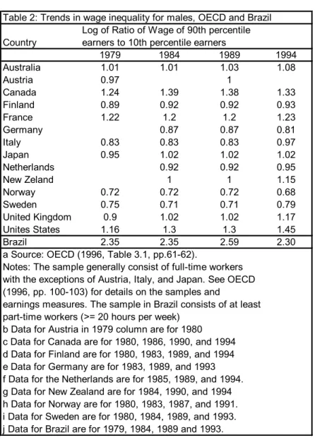
Table 2 shows comparative changes in income inequality in several OECD countries and Brazil. The figures are measured by the log of the wage ratio of the 90th percentile earner to the
10th percentile earner. As may be seen, earnings inequality reaches significant levels in Brazil, compared to the other countries in the sample.
Importantly enough, log wage inter-decile difference was 2.35 in 1979 and only slightly lower in 1993 (2.30). The pattern (a 2.5% fall) seems relatively stable, compared to the increase of 25% in United States during the same period. This stability is merely apparent, however. Earnings inequality increased 10% from 1979 to 1984 and then fell by 12% by 1993. Such ups and downs of income inequality are highly typical for a developing countries that may experience a high level of short run GDP volatility, as is the case in Brazil. Moreover, during most of the sampled period
1 In this draft, I just cover the evolution of the 10th, 50th and 90th percentile of earnings distribution.
2 This table was withdrawn from the appendix in order to fit on the size requirements of ANPEC. It is available from the authourThis is a selective sample drawn from the World Bank study on Income Inequality. Such figures take household level as the unit of analysis, and consider per capita household income, adjusted for the size of the household. The definition of income is rather variable across surveys, with the survey years also showing variation.
Brazil has suffered from high inflation, which helps to make instantaneous earnings less informative about actual individual purchasing power. The paper seeks to investigate the factors driving changes in income distribution in the long run, rather than those related to transitory movements of income inequality.
The level of education has changed dramatically for younger groups entering the labor force. The phenomenon has been captured in other studies3. As an example, the length of schooling for
participating males increased from 4.9 years, in 1977, to 7 years, in 19984. With regard to different generations, someone born in 1920 had an average education of 3.47 years, while those born in 1965 completed an average of 7.5 years of study. Illiterates compound 30% of males born in 1912, against only 3.5% of those born in 1973. The proportion of workers with at least 9 years of study increased from 10.5% to 40%, for the same two groups.
At the same time, educational improvement has been unevenly distributed. The distribution not only suffered a shift upward, but it became more asymmetric towards the top. While the 90th percentile increased by 7 years of study (comparing 1920 and 1965 cohorts), the 10th percentile increased just 2 years. At the same time, the school premium has decreased, mainly for those who completed the intermediary level and those with a high school diploma. Such decrease accentuated during the 1990s5.
The debate on the sources of income inequality in Brazil dates back to the early 1970s. Langoni (1973) is the seminal paper relating earnings and schooling distribution. Contrasting with the period covered in this paper, the economy grew at high rates during the 1960s. The author speculates that such growth was technology-driven, and the demand for high skill workers pushed school premium and educational investment up. By decomposing the log wage variance between price and quantity factors, he presents evidence that the increase in the educational inequality explains about 40% of the overall increase in income inequality, for the period 1960-70.
An important reference in the debate on the effects of changes in educational distribution on earnings distribution is Lam & Levison (1992). They find disturbing the increase in earnings inequality from 1976 to 1985, in face of the general fall in educational inequality. As we show, their sample period suffers a substantial impact of inflation on earnings dispersion. Their optimistic forecast that the stronger educational convergence among younger generation would decrease future earnings inequality was not confirmed by the data. Particularly, the increase in education dispersion among the 50% poorer has contributed to a positive net effect of education endowment on earnings inequality. Moreover, school premium fall has been the most important source driving overall earnings inequality down, especially during the 1990s. The behavior of school distribution, however, is important to explain the upward skewness on earnings distribution during the period of analysis.
The rest of the paper is divided into seven sections. Section 2 presents the database, a panel of nationwide household surveys. Section 3 presents general figures for income and educational performance by cohort and by year. In section 4, exercises of income inequality decomposition and simulation are carried out. The approach developed by JUHN et al. (1993) is applied in order to determine how much of the changes in inequality are due to variation in skill returns, how much
3 See PASTORE & SILVA (1999) and BARROS, MENDONCA & SANTOS (1999), as examples.
4 Throughout this paper, only earnings of males are considered, since these populations did not suffer any significant changes in their participation patterns. In the case of women, the decision as to whether to take part in the labor force has shifted. As an example, an incomparable large proportion of highly educated women is entering the labor now. In this way, a higher average school level for workers may partly be driven by this type of decision, rather than because women are studying more.
5 Possible reasons for the reduction in school premium are a supply effect (increase in supply of high school graduates) and a demand effect (trade liberalization or technologic shocks). Example of paper following the first approach is Ferreira (2002). Evidence of papers following the second approach are Gonzaga et al. (2002), among others.
to changes in actual education distribution and how much is due to residual (within-group) inequality. In addition, it is possible to simulate de impact of quantities and prices in different segments of the labor earnings distribution. Section 5 presents conclusions.
Table 2: Trends in wage inequality for males, OECD and Brazil Log of Ratio of Wage of 90th percentile Country earners to 10th percentile earners
1979 1984 1989 1994 Australia 1.01 1.01 1.03 1.08 Austria 0.97 1 Canada 1.24 1.39 1.38 1.33 Finland 0.89 0.92 0.92 0.93 France 1.22 1.2 1.2 1.23 Germany 0.87 0.87 0.81 Italy 0.83 0.83 0.83 0.97 Japan 0.95 1.02 1.02 1.02 Netherlands 0.92 0.92 0.95 New Zeland 1 1 1.15 Norway 0.72 0.72 0.72 0.68 Sweden 0.75 0.71 0.71 0.79 United Kingdom 0.9 1.02 1.02 1.17 Unites States 1.16 1.3 1.3 1.45 Brazil 2.35 2.35 2.59 2.30
a Source: OECD (1996, Table 3.1, pp.61-62).
Notes: The sample generally consist of full-time workers with the exceptions of Austria, Italy, and Japan. See OECD (1996, pp. 100-103) for details on the samples and
earnings measures. The sample in Brazil consists of at least part-time workers (>= 20 hours per week)
b Data for Austria in 1979 column are for 1980 c Data for Canada are for 1980, 1986, 1990, and 1994 d Data for Finland are for 1980, 1983, 1989, and 1994 e Data for Germany are for 1983, 1989, and 1993 f Data for the Netherlands are for 1985, 1989, and 1994. g Data for New Zealand are for 1984, 1990, and 1994 h Data for Norway are for 1980, 1983, 1987, and 1991. i Data for Sweden are for 1980, 1984, 1989, and 1993. j Data for Brazil are for 1979, 1984, 1989 and 1993.
2- Data
The data are drawn from the Brazilian Nationwide Household Sample (PNAD), for the years 1976-986. Only males are selected from this sample, with women excluded due to the substantial change in the participation of this group in the labor force over the last two decades.
Additionally, only individuals aged more than 24 are considered, with the aim selecting only individuals who had already completed their formal education cycle. Late college graduation is a factor that causes underestimation of the proportion of college graduates among very young cohorts. Only individuals aged 64 or less are considered in the sample in order to remove potential
6 Data is not available for the following years: 1980, 1991 and 1994. The first two periods were census years and a strike in IBGE caused the interruption of the series in 1994.
sample composition bias. Public old age benefits in Brazil produces incentives to early retirement, especially for successful individuals7.
The sample is conditioned on at least part-time employment (20 hours per week) in all jobs8. Hence, unemployed (or non-participating) persons are excluded from the sample9. The nominal wage was constructed by dividing usual before-tax monthly earnings (the income reported by the individual to the questionnaire) by monthly hours for the reference week10. Only self-employed or
employed individuals are considered11, as are only employees in non-agricultural jobs12, and urban areas.
I exclude individuals who earn very low or extremely high wages, which are likely to be consequence of measurement errors. The core sample is restricted to workers who earned at least R$ 6 a week in 1996 monetary unit (equal to a quarter of the 1996 real minimum wage based on a 40-hour week)13, and at most some year-specific value, defined according to the sample distribution for each year14. The remaining sample size is 885,475 observations.
Formal educational attainment is measured by the highest grade reached by the individual. Unfortunately, the variable is partly a category and partly a numerical one. For 8 years of study or less, PNAD gives the exact number of years studied (in fact, the number of years corresponding to the highest grade achieved by the individual). For the secondary level, PNAD only indicates whether the worker studied at least until the 9th grade and at most up to the 11th grade. The sample years 1977 and those after 1992 are exceptions for which the full set of schooling years is specified. The same applies to college students, where it is not clear whether individuals
7 Estimates of age-wage profile do not suffer any significant change if only individuals aged less than 60 are considered. The exclusion of non-participating males is a minor problem provided that the sample does not contain too young or too old individuals. The idea of focusing only on individuals aged over 24 and under 65 intends to address this selection problem. 8 The total working hours is obtained by summing the number of hours worked in each job. For example, one individual working 10 hours a week in job A and other 10 hours in job B will be included in the sample as working 20 hours a week.
9 Excluding the unemployed may introduce some composition bias, particularly during recession years in which unemployment usually increases substantially, affecting mainly low skill workers. In general, the exclusion of unemployed males, which are effectively supplying labor, might introduce some bias in this distribution, if low skill workers, for example, have lower probability to find a job. Little can be done to correct for this composition bias here. Such individuals are excluded since it is possible to observe their wages. A factor that attenuates potential bias is the inclusion within the sample of self-employed. In developing countries, as Brazil, informal self-employment works as an income buffer during recessions.
10 Non-wage employee benefits, such as employer pension contributions and employer-provided health insurance represent a significant share of total (pecuniary) compensation in Brazil, at least for those with higher education. Transportation and food vouchers (supplied by the employer) represents an important share of total compensation for low skill jobs. Nonetheless, the household survey does not account for such fringe benefits. Thus, the paper considers hourly wage the unique source of labor earnings.
11 This implies the exclusion of employers (entrepreneurs) and all kind of non-remunerated work. It is important to consider self-employment in Brazil, since a reasonable share of low skilled people have such jobs (working on street carts, for example). Additionally, part of the sample of employees consists of informal workers (whose employers do not pay payroll tax and other payroll related contributions).
12 Agriculture jobs are excluded since an important part of the wage is paid in kind (i.e. not monetary). Moreover, there are strong seasonal factors that determine wages. Since it was not possible to obtain average annual earnings, but only earnings for a specific week, seasonal factors would introduce a substantial bias into the estimators used here.
13 Nominal wages are converted into constant dollars using GPI-FGV between 1976 and 1978, and CPI-IBGE, between 1979-98. 14 The upper bound from 1983 to 1998 is R$ 719.00 per hour, or R$ 28.76 a week (assuming a 40 hour week). This represents respectively the percentile: 98.43%, in 1998; 98.63%, in 1997; 98.25%, in 1996; 98.77%, in 1995; 99% in 1993; 99% in 1992; 99.25% in 1990; 99.25% in 1989; 99.11% in 1988; 99.49% in 1987; 99.44% in 1986; 99.54% in 1985; 100% in 1984 and 1983. The other upper bounds, and respective percentiles in the unrestricted distribution are, in hourly terms: R$ 190.00 (99.7%), in 1982; R$ 177.00 (99.7%), in 1981; R$ 154.00 (99.78%), 1979; R$ 262.00 (99.82%) in 1978; R$ 393.00 (99.81%) in 1977; R$ 971.00 (99.71%), in 1976. The aim of such upper boundaries was to eliminate unrealistic earnings reports. Such misreporting is easy to identify, since there is enormous discontinuity above the cutoff points, with the next value being as much as 100,000 larger than the chosen cut-off point. Such misreported data occurred in more than 1.75% of the sample in recent years, with a much smaller fraction for the data from the 1970s.
graduated or not, and if not, how many years they took (again, the exceptions are 1977 and the years after 1992).
Cohort variable is defined by the year of birth. Since the sample includes only individuals aged between 25 and 64, some of the cohorts are not present in every year. For example, individuals aged 25 in 1998 were only 3 years old in 1976, and are not present in the 1976 sample.
3 - Stylized Facts:
3.1) Income Inequality: 1976-1998
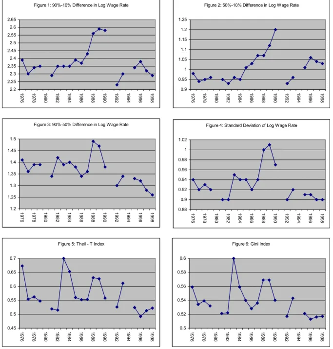
Figures 1 to 3 present the evolution of earnings inequality, using inter-decile differences in log wage rate15, which has been highly unstable, especially during the second half of the 1980s, partly on account of nominal shocks. As is well known, price and wage dispersion increases during high inflation (as a result of unsynchronized nominal adjustment). Hence, periods marked by high variation in inflation cause greater income inequality16. However, such shocks are transitory and do not affect the long-term pattern of earnings. Thus, it is more important to identify low frequency movements in earnings dispersion.
In 1976, the hourly wage rate of the 90th percentile was 10.9 times higher than the hourly wage of the 10th percentile. The difference fell to 9.8 (10% decrease), in 1998. The difference between
the median earner and the 10th percentile poorest increased during this period (from 2.7 to 2.8, which is a 5% increase). The decrease in income inequality occurred among the top 50th earners. The 90th percentile richest got, in 1976, 4 times the 50th, and 3.5 times in 1998, which represents a 14% fall in wage inequality. As the figure 3 shows, the difference between the top 90th earner and the median earner has fallen systematically, with a clear negative trend over the years. The hypothesis of tested on this paper is that such movement of earnings distribution replicates, in part, the shifts in educational distribution. As we will see, both wage and education distributions are becoming skewed, upward biased.
Inter-decile differences have the inconvenient characteristic of ignoring values in the upper and lower tail of the distribution. Figures 4 and 5 analyze income inequality by looking at estimators of the Generalized Entropy Class. Figure 4 shows the standard deviation of log wage rate and
figure 5 shows the Theil T index17. The standard deviation of log wage rate shows a reduction on the labor earnings dispersion from 0.93 in the 1970s to 0.91 in the 1990’s. Both the Theil and Gini Indexes show similar patterns of income inequality, with a slight reduction in income inequality during the 1990s, when compared with the second half of the 1970s, and a huge decrease when compared to the 1980s. Table 3 shows the general picture, over a 5-years period.
All these movements are being captured for a period during which Brazil’s economic performance was poor, as highlighted by data on real wages. The median worker earned, in 1996 monetary units, R$ 2.32 per hour in 1976 and R$ 2.36 per hour 22 years later.
3.2) Educational Performance:
The distribution of formal educational attainment has been shifting toward the highest grades for Brazilian workers born in the 20th century, as may be inferred from the comparison among cohorts, in Figure7. The main characteristics of the figure are:
15 It is important to make some comments about the difference between the measures of income inequality. It is well known that variance of log wage is a useful summary measure of wage dispersion if wages are approximately log normal, but is much more sensitive to extreme outliers at the top and at the bottom than are the quantile measures of wage dispersion. Income inequality, measured by variance of log wage presents the same trend slightly downward, but have more marked kinks for the periods of high inflation.
16 Earnings questions in the PNAD survey refer to “last month labor income in all jobs”. Different unsynchronized adjustments can make a big difference in earnings between two persons getting exactly the same average wage.
1) the continuing fall in illiteracy rates, from 30% for the generation born in 1912 to 3.5% for those born in 1973;
2) the huge increase in the percentage of workers with at least one complete high school year, from 4% for those born in 1912, to 30% for those born in 1973;
3) Intermediary grade attainment that rises and then falls. The percentage of workers for which the highest degree attained is the 4th (complete primary school), increases up to cohorts
born in 1935, and then falls dramatically (at the same time as the proportion of those who completed the 8th grade increases).
Figure 1: 90%-10% Difference in Log Wage Rate
2.2 2.25 2.3 2.35 2.4 2.45 2.5 2.55 2.6 2.65 1976 1978 1980 1982 1984 1986 1988 1990 1992 1994 1996 1998
Figure 2: 50%-10% Difference in Log Wage Rate
0.9 0.95 1 1.05 1.1 1.15 1.2 1.25 1976 1978 1980 1982 1984 1986 1988 1990 1992 1994 1996 1998
Figure 3: 90%-50% Difference in Log Wage Rate
1.2 1.25 1.3 1.35 1.4 1.45 1.5 1976 1978 1980 1982 1984 1986 1988 1990 1992 1994 1996 1998
Figure 4: Standard Deviation of Log Wage Rate
0.88 0.9 0.92 0.94 0.96 0.98 1 1.02 1976 1978 1980 1982 1984 1986 1988 1990 1992 1994 1996 1998
Figure 5: Theil - T Index
0.45 0.5 0.55 0.6 0.65 0.7 1976 1978 1980 1982 1984 1986 1988 1990 1992 1994 1996 1998
Figure 6: Gini Index
0.5 0.52 0.54 0.56 0.58 0.6 1976 1978 1980 1982 1984 1986 1988 1990 1992 1994 1996 1998
4) The percentage of college graduates rises for cohort born up to and including 1955, and then starts to fall. The reason for the fall seems to be that part of the true population of students is excluded from the sample, as such individuals are still completing their grade (and so opting to be
out of the labor force)18. In other words, late graduation is the only factor that explains the decrease in the share of college graduates for the very young cohorts.
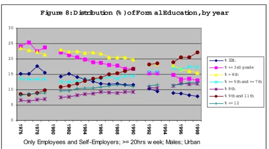
5) The analysis, by year, reveals the same trend of educational improvement, as is shown in
Figure 8.
Table 3
Measures of wage inequality for weekly wages of full time male workers, PNAD, 1976-1998
SD of log wage Percentile of log wage distribution Gini Coefficient Theil T
90-10 90-50 50-10 1978 0.93 2.34 1.39 0.95 0.539 0.562 1983 0.95 2.35 1.39 0.96 0.600 0.700 1987 0.94 2.43 1.36 1.07 0.536 0.553 1993 0.92 2.30 1.34 0.96 0.543 0.611 1998 0.90 2.29 1.26 1.03 0.517 0.522
OBS: Upper bounds are :
R$ 719.00 from 1983 to 1998. R$ 190.00 in 1982 R$ 177.00 in 1981 R$ 155.00 in 1979 R$ 263.00 in 1978 R$ 394.00 in 1977 R$ 972.00 in 1976 Lower Bound is: R$ 0.15, for all years
All figures are in 1996 values, and represent earnings per hour.
Figure 7: D istribution of Form al Education, by C ohort
0 5 10 15 20 25 30 35 40 % illit. % <= 3rd grade % = 4th % >= 5th and <= 7th % 8th % 9th and 11th % >= 12
Only Employees and Self-Employers; >= 20hrs w eek; Males; Urban
18
Late college graduation may distorts downward the proportion of college graduates for younger cohorts. Because non-participating males are excluded from the sample, and because a high contingent of youths are still in college (and so out of the labor force), the reduction of workers with at least 12 schooling years is expected to fall, if late graduation is an issue. The sample problem introduced by late graduation is attenuated partly if we restrict the sample to individuals older than 30. For example, 13% of workers born in 1965 in this restricted sample have college degree, while only 11.9% in the unrestricted sample (including workers older than 25).
Figure 8: D istribution (% ) of Form al Education, by year 0 5 10 15 20 25 30 % illit. % <= 3rd grade % = 4th % >= 5th and <= 7th % 8th % 9th and 11th % >= 12
Only Employees and Self-Employers; >= 20hrs w eek; Males; Urban
Although this sample does not represent the entire male population19, it captures the outstanding increase in the average level of education, and the decrease in the dispersion of educational distribution in Brazil.
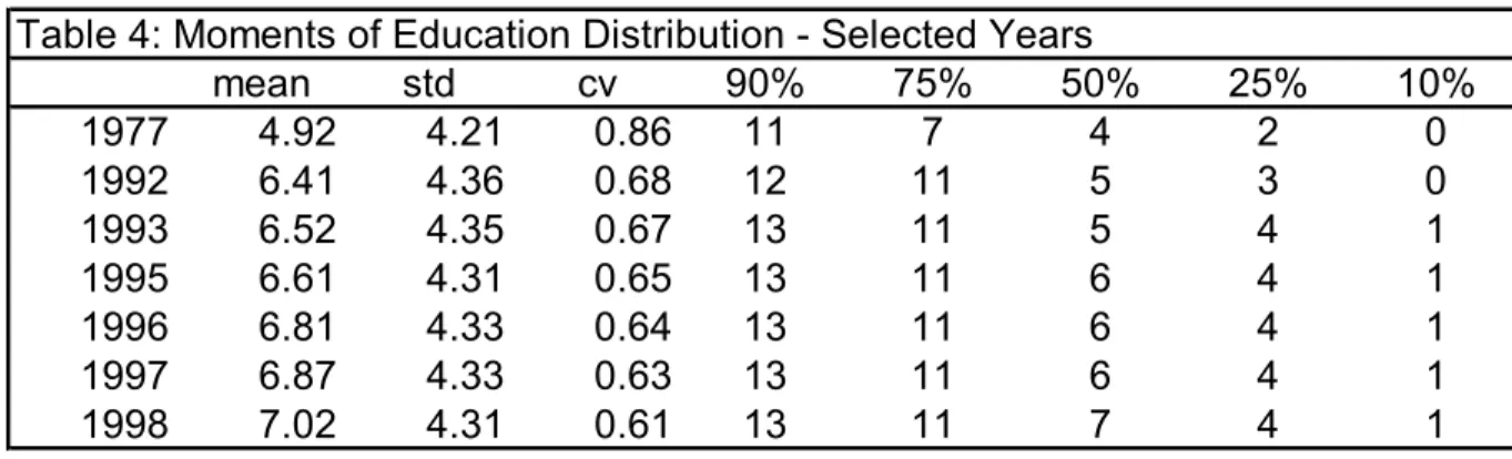
Table 4 below shows that the increase in the educational level has been concentrated in the top percentiles of the distribution20. The top 90th percentile has two more years of education in 1976 than in 1998. At the 75th percentile years of education increased by impressive 4 years over the same period of time, while the median student went from 4th grade (completed primary level) to
7th grade. This indicates that the difference in those at the top of the distribution has contracted. At the same time, the inter-decile difference between the 90th and the 10th decile increased by one year. In particular, the performance of the 10th decile was poor, rising from illiteracy to just one
year of school. The distance between the 75th percentile and the 10th percentile increased from 7 to 10 years of school, which reaffirms an unequal educational performance in the population.
Since 1977, the mean educational attainment of individuals aged between 25 and 64 years old, living in urban neighborhoods, and working more than 20 hours a week increased from 4.9 years of school to 7 years. The coefficient of variation has decreased from 0.86 to 0.61. The Gini and the Theil indexes for school years show the same pattern, falling mildly.
Repeating the above analysis for selected cohort groups (Table 5), one can see that the average number of school years goes from 3.5 (for the generation born in 1920) to 7.5 (for workers born in 1968). The increase in average education for the cohort born in 1945 (compared to those born 5 years earlier) is especially large.
19 Considering only urban workers is likely to overestimate the share of highly educated individuals, because rural workers in Brazil have a lower level of education.
20 Tables 4 and 5 are based only in the sample years 1977, 1992, 1993, 1995, 1996, 1997 and 1998. For those years, the variable school year is not categorical. Thus, it is possible to know the exact grade of the worker..
Table 4: Moments of Education Distribution - Selected Years mean std cv 90% 75% 50% 25% 10% 1977 4.92 4.21 0.86 11 7 4 2 0 1992 6.41 4.36 0.68 12 11 5 3 0 1993 6.52 4.35 0.67 13 11 5 4 1 1995 6.61 4.31 0.65 13 11 6 4 1 1996 6.81 4.33 0.64 13 11 6 4 1 1997 6.87 4.33 0.63 13 11 6 4 1 1998 7.02 4.31 0.61 13 11 7 4 1
Table 5: Moments of Education Distribution - Selected Generations - 30 <= Age <= 60
Birth mean std cv 90% 75% 50% 25% 10% 1920 3.47 4.03 1.161 8 4 3 0 0 1925 3.85 3.97 1.031 9 4 3 1 0 1930 4.13 4.00 0.969 11 5 3 1 0 1935 4.36 4.13 0.947 11 5 4 1 0 1940 4.70 4.31 0.917 11 7 4 2 0 1945 5.77 4.60 0.797 14 8 4 3 0 1950 6.26 4.51 0.720 15 11 5 3 0 1955 6.94 4.39 0.633 15 11 6 4 2 1960 7.19 4.25 0.591 15 11 7 4 2 1965 7.48 4.08 0.545 15 11 8 4 2 1968 7.50 4.05 0.540 15 11 8 4 2
OBS: Only considers years when the school variable was the exact grade obtained. Those years are: 1977, 1992, 1993, 1995, 1996, 1997, 1998.
Overall education inequality, measured by the coefficient of variation (a mean-independent measure), has been falling for younger cohorts. In fact, even the standard deviation presents an inverted U-shape. The fall in the coefficient of variation of educational distribution matches those found by Lam (1999) and Lam & Levison (1992), who looks only at the evolution by cohort21.
Improvement of education occurred mainly for the upper part of the distribution. The gap in education level between the top 90th and the top 75th has remained constant, while the distance between the number of years studied for the 75th and the 10th percentile has increased. This difference in educational performance, depending on which section of the educational distribution we refer to, suggests that for those at the bottom of the educational distribution there is apparently some difficulty in remaining free from the “illiteracy trap”. While the highly educated individual gained seven years of study from the 1920 to the 1960 cohort (increasing years of study from 8 to 1522), time of schooling for those in the bottom 10% percentile of the educational endowment
distribution increased by only 2 years more in the same period. As one can see, the same upward skewness on earnings distribution is observed on educational distribution.
21 Lam & Levison (1992) find that “decomposition of a standard human capital earnings equation (by cohort) indicates that trends in schooling tended to reduce earnings inequality from 1976 to 1985, due to reductions in both the variance of schooling and in returns to schooling”. In their work, they do not separate between school premium and actual educational distribution effects. In the yearly analysis, the overall schooling inequality has not reduced substantially, even for the period 1976-1985. On contrary, there is evidence that it has contributed to increase earnings inequality among the 50% poorer and to slightly decrease the earnings inequality among the 50% richer. The net effect is a positive contribution to increase earnings inequality, as we will show below. 22 This in fact is an underestimate, since the variable for school years is truncated at 15 (corresponding to a 4-year college or more).
3.3) Income Inequality: different generations
Does such a striking increase in educational attainment tend to reduce inequality? How much of an impact could unequal educational development have in income distribution? What happens to income dispersion for those different generations? Comparing different cohorts requires separating out the effects of time, age and cohort on income dispersion23. It is nevertheless
possible to look at the income distribution for different generations to see if the pattern observed on the educational distribution is repeated in earnings distribution, as is shown in Table 7. Measured in log wages, income dispersion falls by 30% (Gini Index) and 26% (standard deviation), between the older (born in 1920) and the younger generation (born in 1968).
The distance between the top 90th and the top 50th decreased 27%, from cohorts born in 1920 to those born in 1968. In particular, the distance between the 90th percentile wage rate and the 75th narrowed by 31%. The distance between the 50th and the 10th percentile nevertheless decreased by only 9%. This resembles the pattern for educational distribution. Although extremely care is required with such figures (due to time and age effects, and some remaining composition bias), the data is sufficient to motivate a more in-depth study of the impact of educational improvement on income inequality. A definitive answer about such an impact will depend on both the changes in the school premium and in the distribution of education.
Table 7: Moments of Log Wage Distribution - Selected Generations - 30 <= Age <= 60
Birth mean std 90% 75% 50% 25% 10% 90%-50% 50%-10% 90%-10% 90%-75% 75%-10% Gini Theil
1920 0.83 1.07 2.27 1.4 0.69 0.1 -0.34 1.58 1.03 2.61 0.87 1.74 0.647 0.992 1925 0.81 1.03 2.22 1.4 0.68 0.08 -0.37 1.54 1.05 2.59 0.82 1.77 0.610 0.835 1930 0.85 1.01 2.22 1.44 0.74 0.13 -0.33 1.48 1.07 2.55 0.78 1.77 0.589 0.712 1935 0.91 0.99 2.26 1.52 0.8 0.22 -0.28 1.46 1.08 2.54 0.74 1.8 0.564 0.621 1940 0.94 1.00 2.33 1.53 0.84 0.23 -0.24 1.49 1.08 2.57 0.8 1.77 0.573 0.664 1945 1.05 0.99 2.43 1.65 0.95 0.34 -0.16 1.48 1.11 2.59 0.78 1.81 0.562 0.628 1950 0.99 0.96 2.31 1.58 0.91 0.3 -0.18 1.4 1.09 2.49 0.73 1.76 0.550 0.622 1955 1.01 0.94 2.29 1.62 0.94 0.34 -0.17 1.35 1.11 2.46 0.67 1.79 0.521 0.504 1960 0.89 0.89 2.11 1.43 0.81 0.29 -0.2 1.3 1.01 2.31 0.68 1.63 0.503 0.478 1965 0.90 0.86 2.07 1.43 0.83 0.3 -0.14 1.24 0.97 2.21 0.64 1.57 0.492 0.463 1968 0.86 0.79 1.95 1.35 0.79 0.33 -0.15 1.16 0.94 2.1 0.6 1.5 0.450 0.369
OBS: Only considers years when the school variable was the exact grade obtained. Those years are: 1977, 1992, 1993, 1995, 1996, 1997, 1998.
3.4) Skill Premium
How has school premium changed during the last 20 years in Brazil? First, it is important to say that, compared to the United States, school premium in Brazil is high. For example, considering only workers older than 25 years old, the college/high school log wage difference in Brazil was 0.82 in 1976, while just 0.34, in US.
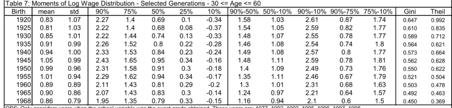
Although the college premium (measured here by the difference between the mean wage for the college group and the mean wage for high school group) increased slightly during this period, the school premium fell for every measure comparing wages of workers with a relatively high education (at least 8th grade) and those with a relatively low education (less than 8th grade). The gap between college graduates and illiterate workers narrowed 13.3%. The wage gap between high school graduates and illiterates was reduced 29%, while the difference between workers that completed the 8th grade and illiterates narrowed by 38%. The gap between high school and 4th grade workers narrowed by 29%. The wage gap between 8th grade and 4th grade workers narrowed 49%, in 22 years. Figure 9 shows the school premiums for some select groups.
One possible hypothesis for a reduction in the skill premium is that it was a consequence of the increasing supply of relatively educated workers. The fact that a significant contingent of high
school graduates entered the labor force generated excessive supply, and a reduction in the school premium of relatively more qualified workers24.
Figure 9: Mean Log Wage Differences for Selected Educational Groups, 1976-1998 0.4 0.5 0.6 0.7 0.8 0.9 1 1976 1978 1980 1982 1984 1986 1988 1990 1992 1994 1996 1998 4th Grade/Illiterates HS/4th grade College/HS
The figure shows how the wage gap between high school and 4th graders narrowed, particularly during the 1990s, when trade liberalization may have caused the reduction in school premium. Heckscher-Ohlin theorem predicts that the country would specialize in producing unskilled-labor intensive goods, while importing skilled-labor intensive goods – since there is relative abundance of the first factor and relative scarcity of the second one (compared to other countries). This would tend to drive down the skill premium. The results here show that the decrease in the wage gap between high school earners and illiterates are possibly a consequence of trade liberalization. This suspection is partly confirmed by other empirical papers25.
One can perform an econometric estimation for each year, controlling for regional and age/cohort effects. The evolution of school premium is, as expected, quite similar to that shown in
Figure 9, although the size of the premium is smaller in the multiple regression. This is mainly an effect of the regional dummy for the richer states. Since most of the low educated workers are in the poor states and most of the highly educated in the rich states, the educational premium would be expected to fall when allowing only for intra-regional variation. The resulting estimates are presented in Table 8, in the appendix.
4) Inequality Decomposition:
By using some simple econometric tools it is possible to determine how much of the explained earnings dispersion (the so-called between-group income inequality) is caused by school premium change and how much may be attributed to the change in quantities. In addition, it is possible to
24 ACEMOGLU (1999) presents a model in which the relative amounts of skills determine the type of jobs offered. In a country where there is shortage of highly skilled workers, the available technology is not skill specific. In such situation, there is a pooling equilibrium, with both high- and low-skill workers being hired for the same job. There is over-investment in education, for some highly educated individuals. As a consequence, skill premium falls as more educated individuals enter the labor force. Above some threshold, however, a screening equilibrium arises. The upgrade in education, with a higher share of highly educated workers, causes firms to change to skill specific technologies. Over-investment in education is eliminated and income inequality increases. Assuming this model is correct, Brazil would be below the threshold, and an educational upgrade causing a fall in school premium and earnings inequality.
25 MESQUITA & NAJBERG (1999) show, using analysis by industry, that unemployment rates increased more for relatively high skill workers, as a consequence of trade liberalization in the 1990s. For recent empirical evidence of trade liberalization and income inequality in the world, see AGHION, CAROLI & GARCIA-PENALOSA (1999).
observe how residual (within-group) inequality has changed over time. This section focuses on applying the appropriate tools to analyze components of earnings inequality changes in Brazil.
4.1) “Between-Group” versus “Within-Group” Inequality
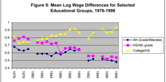
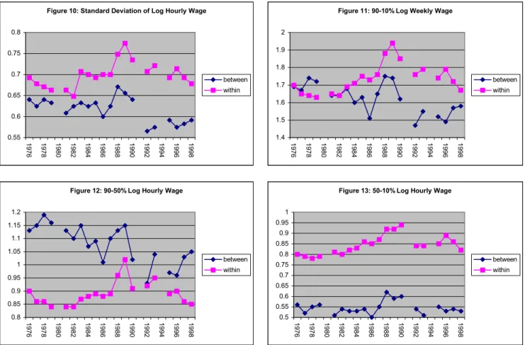
Between-Group inequality is examined here by looking at changes in the distribution of explained log wage from cross-section regressions of log hourly wage on a full set of 10 education dummies, a quadratic polynomial in age, interactions of the age quadratic polynomial with 3 broad education categories and one regional dummy. The within-group inequality is obtained from residual log wage. Figures 10 to 13 track between-group and within-group components of earnings inequality over the 22-year period.
Figure 10: Standard Deviation of Log Hourly Wage
0.55 0.6 0.65 0.7 0.75 0.8 1976 1978 1980 1982 1984 1986 1988 1990 1992 1994 1996 1998 between within
Figure 11: 90-10% Log Weekly Wage
1.4 1.5 1.6 1.7 1.8 1.9 2 1976 1978 1980 1982 1984 1986 1988 1990 1992 1994 1996 1998 between within
Figure 12: 90-50% Log Hourly Wage
0.8 0.85 0.9 0.95 1 1.05 1.1 1.15 1.2 1976 1978 1980 1982 1984 1986 1988 1990 1992 1994 1996 1998 between within
Figure 13: 50-10% Log Hourly Wage
0.5 0.55 0.6 0.65 0.7 0.75 0.8 0.85 0.9 0.95 1 1976 1978 1980 1982 1984 1986 1988 1990 1992 1994 1996 1998 between within
While overall inequality, measured e.g. by standard deviation (figure 4), decreases slightly, this behavior is due apparently to between-group inequality, since residual inequality varies roughly between 0.75 and 0.65 (figure 10). Between-group income inequality narrows significantly for the top 50th percentiles of income distribution. The difference between the 90th and the 50th percentile wage rate falls from about 1.15 in the 1970s to 1 in the 1990s (figure 12). The explained wage gap between the bottom 50%, however, does not show any trend.
Residual inequality increases as a share of overall inequality. While the combination of a lower school premium and more equal school distribution indices lower earnings inequality, the residual inequality is slightly larger in the 1990s than it was in the 1970s. It may be true that part of the change in residual inequality is due to unobserved permanent changes in population characteristics. Such permanent changes in residual inequality could be due to a less homogeneous distribution of school quality within educational groups, although it is not possible to confirm this using the available data. Additionally, residual inequality may be a result of permanent changes in the premium of unobserved skills.
4.2 Screening between quantity and price components of income inequality
How much of the change in the between-group earnings inequality is a result of changes in school premium and how much is a direct effect of the distribution in schooling? The following section applies the full-sample distribution accounting scheme developed by JUHN et al. (1993) to screen the share of the reduction in inequality induced exclusively by the changes in the educational distribution, and the share of variation caused by changes in school premium. This approach begins with a simple wage equation, such as
it t
it
it
X
B
u
Y
=
+
(1)where
Y
it is the log wage of individual i in year t,X
it is a vector of observed individualcharacteristics (e.g. experience and education),
B
t is the vector of estimated (OLS) returns to observable characteristics in t, andu
it is the log wage residual (which depends on price and quantities of unobserved skills, measurement error, and estimation error). This residual has two components: an individual’s percentile in the wage distributionθ
it and the distribution function ofthe residuals
F
t(.)
. By the definition of the cumulative distribution function, we can write the residual as)
|
(
1 it it t itF
X
u
=
−θ
, (2) whereF
1t(.
|
X
it)
−is the inverse cumulative residual distribution for workers with characteristics
X
it in year t.The framework given by equations (1) and (2) decomposes changes in inequality into three sources: (1) changes in the distribution of individual characteristics (changes in the distribution of X’s); (2) changes in the returns to observable skills (changes in the B’s); and (3) changes in the distribution of residuals. By defining
β
as the average returns to observable variables over the whole period under study andG
(.
|
X
it)
to be the average cumulative distribution, we can decompose the level of inequality into corresponding components using)]
|
(
)
|
(
[
)
|
(
)
(
1 1 1 it it it it t it it t it it itX
X
G
X
F
X
G
X
Y
=
β
+
β
−
β
+
−θ
+
−θ
−
−θ
. (3)The first term captures the effect of changing distribution of worker characteristics; the second measures the effects of changing skill returns; and the third term accounts for changes in the distribution of the residuals. This framework allows one to reconstruct the (hypothetical) wage distribution that attainable with any subset of the components held fixed. One does not need to hold any of the components fixed at the average level for the entire sample. It is enough to simulate hypothetical wage distributions using any base period and replace
β
and)
|
(.
X
itG
with the values for a reference period of interest.If observable skill returns and the residual distribution were held fixed so that only observable quantities are allowed to vary, then wages would be determined by
)
|
(
1 1 it it it itX
G
X
Y
=
β
+
−θ
. (4)If observable skill returns and quantities are allowed to vary over time with only the residual distribution held fixed, then wages are generated by
)
|
(
1 2 it it t it itX
G
X
Y
=
β
+
−θ
. (5)The recommended approach of JUHN et al. (1993) is to calculate the distributions of
Y
it ,1
it
Y
andY
it2 for each year studied and to attribute the change over time in the1 it
Y
distribution to changes in observable quantities. Any additional change in inequality inY
it2 beyond inequality changes inY
it1 is attributed to observable skill returns. Further change in the actual overall inequality ofY
it beyond those found in2
it
Y
is attributed to changes in the distribution of residuals.I perform separate regressions by year of log hourly wage on a full set of 10 education dummies, with the base year 1981. It is straightforward to show that changes in the total distribution
Y
it−
Y
i81 with respect to the base year can be decomposed by three terms:changes in the residual distribution
(
Y
it−
Y
it2)
; changes in the earnings distribution caused exclusively by school premium variation(
Y
it2−
Y
it1)
and changes in the earnings distribution caused by shifts in the schooling distribution(
181)
1
i
it
Y
Y
−
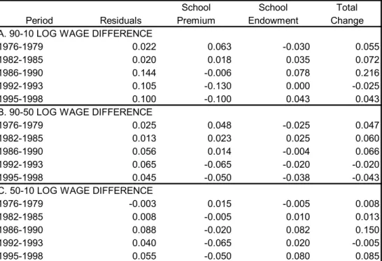
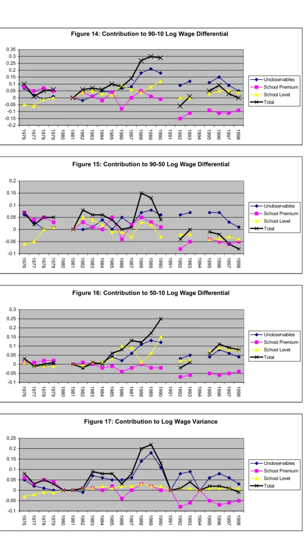
.Figure 14 shows the decomposition of the change in 90th –10th percentile log wage differences, with respect to the base year 198126. In 1998, the last year of the sample, the income inequality was exactly equal to that in 1981. The fall in school premium contributed to reduce it in 0.1 log points. This change was nevertheless exactly compensated by a positive 0.05 contribution in both school level and residuals distributions. The bulk of the middle of the picture corresponds to the hyperinflation period, during which (the second half of the 1980s), school distribution became more dispersed, contributing positively to an increase in inequality. Identification of permanent and transitory (driven by changes in unemployment rates, by school groups) effects on the school distribution cannot be identified here. However, by observing Table 9, it is possible to say that part of the worsening in education distribution was not transitory. The average of log wage difference between the 50-10th percentile, related exclusively to school distribution, is roughly the same for the 1986-1990 and 1995-1998 periods. In other words, if skill premium and residuals had been kept constant at the level of 1981, the earnings inequality in both periods among the 50% poorer would be 0.08 log points higher than in 1981 (measured by log wage differences)27.
Figure 15 shows a negative trend in 90-50th percentile log wage difference, driven by both the reduction in school premium and improved distribution of school endowment among the 50% richer. If premium and residuals are kept at their 1981 level, the log wage difference between the
26 The choice of other base periods (e.g. 1977) did not imply any significant change on those patterns.
27 Ferreira & Barros (2001) perform a more complex decomposition, where they endogenize labor incomes, individual occupational choices and education decisions.
90th and the 50th percentile decreases 0.004 in 1986-90 and 0.038 in 1995-98. Keeping school and residual distribution constant at their 1981 profiles implies that earnings inequality would have fallen 0.014 in 1986-90 and decreased 0.05 in 1995-98, which corresponds to the effect of the observed decrease in school premium.
The average contribution of each component of income inequality, by group of years, shows the increase in the residual earnings dispersion after 1986. If education distribution and skill premium are kept at their 1981 level, changes in the residual distribution are responsible for a increase of 0.02 in overall earnings inequality in 1976-1985, 0.144 in 1986-90 and 0.10 in 1992-1998.
TABLE 9: AVERAGE CONTRIBUTIONS, BY PERIOD
OBSERVABLE AND UNOBSERVABLE COMPONENTS OF CHANGES IN INEQUALITY
School School Total
Period Residuals Premium Endowment Change
A. 90-10 LOG WAGE DIFFERENCE
1976-1979 0.022 0.063 -0.030 0.055
1982-1985 0.020 0.018 0.035 0.072
1986-1990 0.144 -0.006 0.078 0.216
1992-1993 0.105 -0.130 0.000 -0.025
1995-1998 0.100 -0.100 0.043 0.043
B. 90-50 LOG WAGE DIFFERENCE
1976-1979 0.025 0.048 -0.025 0.047
1982-1985 0.013 0.023 0.025 0.060
1986-1990 0.056 0.014 -0.004 0.066
1992-1993 0.065 -0.065 -0.020 -0.020
1995-1998 0.045 -0.050 -0.038 -0.043
C. 50-10 LOG WAGE DIFFERENCE
1976-1979 -0.003 0.015 -0.005 0.008
1982-1985 0.008 -0.005 0.010 0.013
1986-1990 0.088 -0.020 0.082 0.150
1992-1993 0.040 -0.065 0.020 -0.005
1995-1998 0.055 -0.050 0.080 0.085
The decrease in the school premium has been the main driving force behind the fall in general earnings inequality, especially during the 1990s. In the 1970s, school premium contributed positively to income inequality using variance or any percentile difference. However, these contributions become strongly negative during the 1990s.
Educational distribution contributed negatively to income inequality, during the seventies, mainly because, below the median earner, a large contingent of illiterates contributed to make the educational endowment “well distributed”. During the 1980s, unequal advance of schooling explains why school distribution is an important component of earnings inequality for the lower 50% of earnings distribution (oscillating in the range between 0 and 0.15) and is a approximately neutral factor for those above the median earners (oscillating in the range between –0.05 and 0.05). During the nineties, education endowment maintains the same positive contribution to income inequality in the lower range, but drives down earnings inequality for the upper 50%. Hence, for the upper part of the earnings distribution (top 50%), during the 1990s both a decrease in school premium and a better distribution of education across individuals contribute to the fall in the 90-50th percentile log wage difference. For the lower 50%, skill premium falls, but a highly unequal educational endowment is responsible for an increase in earnings inequality.
Figure 14: Contribution to 90-10 Log Wage Differential -0.2 -0.15 -0.1 -0.05 0 0.05 0.1 0.15 0.2 0.25 0.3 0.35 1976 1977 1978 1979 1980 1981 1982 1983 1984 1985 1986 1987 1988 1989 1990 1991 1992 1993 1994 1995 1996 1997 1998 Unobservables School Premium School Level Total
Figure 15: Contribution to 90-50 Log Wage Differential
-0.1 -0.05 0 0.05 0.1 0.15 0.2 1976 1977 1978 1979 1980 1981 1982 1983 1984 1985 1986 1987 1988 1989 1990 1991 1992 1993 1994 1995 1996 1997 1998 Unobservables School Premium School Level Total
Figure 16: Contribution to 50-10 Log Wage Differential
-0.1 -0.05 0 0.05 0.1 0.15 0.2 0.25 0.3 1976 1977 1978 1979 1980 1981 1982 1983 1984 1985 1986 1987 1988 1989 1990 1991 1992 1993 1994 1995 1996 1997 1998 Unobservables School Premium School Level Total
Figure 17: Contribution to Log Wage Variance
-0.1 -0.05 0 0.05 0.1 0.15 0.2 0.25 1976 1977 1978 1979 1980 1981 1982 1983 1984 1985 1986 1987 1988 1989 1990 1991 1992 1993 1994 1995 1996 1997 1998 Unobservables School Premium School Level Total
Residual distribution has similar impacts on both sections of earnings distribution. Residuals distribution contributes positively to income inequality (compared to the base year 1981), with a high impact for the second half of 1980s. The relative symmetry of the residual distribution implies that education endowment is the main factor behind the increasing skewness of earnings distribution, during the 1980s and 1990s.
5. Conclusions:
The main conclusions are:
1) Educational distribution has observed an upward shift in the last 22 years. In particular, high school graduates have increased substantially as a proportion of the younger generations.
2) School premium has decreased substantially, mainly during the 1990’s, for the intermediate school level. Earnings inequality has been decreasing, particularly for the upper part of the earnings distribution. In particular, the difference between the earning rate for the 90th and 50th percentiles has fallen systematically. The bottom 50% of the distribution remains roughly unequal.
3) For the upper part of the distribution, school premium and endowment distribution jointly contribute to decrease income inequality (fall in the school premium and less unequal education endowments), compared to 1981. For the lower part, school premium has contributed negatively to earnings dispersion while (more unequal) school endowments have offset the school premium effect.
4) Residual (or within-group) inequality has varied substantially, especially during the second half of the 80’s (hyperinflation period), without any clear trend. The distribution of shocks is approximately symmetric for every year.
The exercise above seem to tell us that the driving force of reducing income inequality has been an effect of lower school premium, and that this effect was stronger during the 1990s. School distribution has caused dispersion of earnings for the lower part of the income distribution, while leading to the opposite for the upper part of the income distribution. What could explain such apparently different behavior of school endowment on the two parts of the income distribution? As we showed in section III, one hypothesis is that the extension of intermediate public school through the population did not reach those in the lower percentile of schooling distribution. High opportunity cost of human capital investment activities and presence of liquidity constraint could explain the poor education performance of those in the left tail of the educational distribution. It follows that earnings dispersion is worsening for those at bottom 50% of the earnings distribution. All workers in the top 50% are off the education trap. It follows that education will be more homogeneously distributed for those workers, and earnings inequality will be smaller.
8- References:
Acemoglu, Daron. “Changes in Unemployment and Wage Inequality: An Alternative Theory and Some Evidence”. American Economic Review, 1999, vol. 89, no. 5.
Aghion, Philippe, Eve Caroli and Cecilia Garcia-Penalosa. “Inequality and Economic Growth: The Perspective of the New Growth Theories”. Journal of Economic Literature, 1999, vol. 37, Dec.
Angrist, Joshua & Acemoglu, Daron – “How large are the Social Returns to Education? Evidence from Compulsory Schooling Laws” – NBER Working Paper 7444. 1999
Barros, Ricardo, Rosane Mendonca and Daniel Santos. “Uma Analise do Desempenho da Educacao Media no Brasil” – IPEA – 1999.
Bravo, David and Alejandra Marinovic. “Wage Inequality in Chile: 40 Years of Evidence”.mimeo. 1999.
Deaton, Angus and Christina Paxson. “Saving, Growth, and Aging in Taiwan”. In “Studies in the Economics of Aging”, by David Wise. University of Chicago Press. 1992
Ferreira, Francisco & Ricardo Barros. “The slippery slope: explaining the increase in extreme poverty in Urban Brazil, 1976-1996, Revista de Econometria, 1999.
Ferreira, Sergio. “The provision of education and its impacts on college premium in Brazil”, mimeo.
Firpo, Sergio. “Evolucao da Desigualdade de Renda e Consumo entre Familias no Brasil: uma analise de coorte”. Master Dissertation. PUC-RJ. 1999
Gonzaga, Gustavo, Naercio Menezes & Cristina Terra (2002) – Trade liberalization and the evolution of skill earnings differential in Brazil – mimeo.
Heckman, James and Richard Robb. “Alternative Identifying Assumptions in Econometric Models of Selection Bias.” In Advances in Econometrics, vol.5, edited by Truman Bewley. Cambridge University Press, 1987.
Jovanovic, Boyan and Rafael Rob. “The Growth and Diffusion of Knowledge”. Review of Economic Studies, 56, 1989.
Juhn, Chinhui, Kevin Murphy and Brooks Pierce. “Wage inequality and the rise in returns to skill”. Journal of Political Economy , 101, 1993.
Katz, Lawrence and David Autor. “Changes in the Wage Structure and Earnings Inequality”. Handbook of Labor Economics, Volume 3, Edited by O. Ashenfelter and D. Card. Elsevier Science. 1999.
Lam, David. “Generating Extreme Inequality: Schooling, Earnings, and Intergenerational Transmission of Human Capital in South Africa and Brazil”. Mimeo. University of Michigan, Ann Arbor. 1999.
--- and Deborah Levison. Idade, experiência, escolaridade e diferenciais de renda: Estados Unidos e Brasil. Pesquisa e Planejamento Economico, v.20, n.2, 1990.
---. Declining inequality in schooling in Brazil and its effects on inequality in earnings. Journal of Development Economics 37, 1992.
Langoni, Carlos. “Distribuição de Renda e Desenvolvimento Econômico no Brasil”, Rio de Janeiro, Ed. Expressão e Cultura. 1973.
Leal, Carlos and Sergio Werlang. “Retornos em educação no Brasil: 1976/89”. Pesquisa e Planejamento Economico, v.21, n.3, 1991.
Meguir, Costas and Edward Whitehouse. “The Evolution of Wages in the United Kingdom: Evidence from Micro Data”. Journal of Labor Economics, 1996, vol.14, no. 1.
Menezes, Naércio, Reynaldo Fernandes and Paulo Piccheti. “The Distribution of Male Wages in Brazil: some stylized facts.”mimeo. Universidade de São Paulo. 1998.
Moreira, Mauricio and Sheila Najberg. “O Impacto da Abertura Comercial sobre o Emprego: 1990-1997”. In “ A Economia Brasileira nos Anos 90”. By Giambiagi, Fabio and Mauricio Mesquita. Rio de Janeiro. BNDES. 1999.
Psacharopoulos, George and Ana Maria Arriagada. The educational composition of the labor force: an international comparison, International Labor Review 125, No. 5, 1986.
Ram, Rati. “Educational expansion and schooling inequality: iinternational evidence and some implications. Review of Economics and Statistics 72, No. 2, 1990.
Ramos, Lauro and José G. A. Reis. “Distribuição da Renda: Aspectos Teóricos e o Debate no Brasil”. In “Distribuição de Renda no Brasil” by Camargo, José and Fábio Giambiagi. Paz e Terra, São Paulo, 1991.
Reis, Jose G. A. and Ricardo Barros. “Wage inequality and the distribution of education: a study of the evolution of regional differences in inequality in metropolitan Brazil”. Journal of Development Economics, 36, 1991.