U n i v e r s i t y o f H e i d e l b e r g
Discussion Paper Series No. 483 Department of Economics
Efficiency of Public Goods Provision in Space
Travis Warziniack
Title: Efficiency of Public Goods Provision in Space Author: Travis Warziniack
Travis Warziniack (email:Warziniack@eco.uni-heidelberg.de) is a junior professor at the University of Heidelberg, 69115 Heidelberg, Germany. He studies environmental
economics, land use, and general equilibrium modeling.
Corresponding author: Travis Warziniack, Department of Environmental Economics, Alfred Weber Institute, University of Heidelberg, Bergheimer Strasse 20, 69115
Heidelberg, Germany; phone: +49 (06221) 54-8012; fax: +49 (06221) 54-8020; email: warziniack@eco.uni-heidelberg.de
Efficiency of Public Goods Provision in Space
Travis Warziniack Alfred Weber Institute University of Heidelberg
Bergheimer Strasse 20 69115 Heidelberg, Germany warziniack@eco.uni-heidelberg.de
Abstract
This article incorporates a political decision process into an urban land use model to predict the likely location of a public good. It fills an important gap in the literature by modeling the endogenous location of open space. The article compares open space decisions made under a majority-rules voting scheme with welfare-improving criterion and finds households tied to a location in space compete against each other for public goods located nearer them. Significant differences emerge between the two decision criteria, indicating that requiring referenda for open space decisions is likely to lead to inefficient outcomes. Specifically, many open space votes are likely to fail that would lead to welfare improvements, and any open space decisions that do pass will require amenities larger than needed to achieve the social optimum. The more dispersed and large the population, the larger is the gap between the socially efficient level and the level needed for a public referendum to pass.
Much of this work was done during the author’s graduate years at the University of Wyoming with partial funding from the USEPA GRO Fellows program. The USEPA has not officially endorsed this work or the opinions contained within. Many thanks to Ed Barbier, Jason Shogren, David Finnoff, John Tschirhart, Roger Coupal, Aaron Strong, and numerous seminar participants for comments and suggestions.
This article examines the provision of public goods in an urban area and the effect voting has on the level and location of amenities throughout a city. I find significant welfare losses associated with voting for a public good in space. Small public projects that would lead to community-wide welfare improvements are always underprovided, amenities from any public good provided exceed the social optimum, and amenities throughout the city are inappropriately located.
Urban amenities refer to city parks, libraries, recreation and cultural centers, museums, landscaping, and other goods that are publicly provided to for the enjoyment of residents. Parks and recreation centers serve as extended backyards, community gathering places, and wildlife habitat. Cultural centers and landscaping enhance local neighborhoods and are used as a gauge of a community's quality of life. Often these amenities are created by public referendum or by public servants acting on behalf of the community, presumably as if there was a referendum, and, once created, are financed through property taxes spread evenly across the community. The benefits of urban amenities, however, do not accrue evenly across a community. They create a spatial externality in the sense that residents living nearer the public good benefit more than a resident living across town. This introduces two opposing forces in the decision of public good location. There is pressure for amenities to be created where access is highest and spillovers are largest; however, such land is typically more expensive, leading to a higher tax burden.
Ledyard and Palfrey (2002) show that with a large number of individuals, the efficiency of referenda on public goods is similar to mechanisms such as the Lindahl-Samuelson mechanism that achieve the socially efficient outcome. Furthermore,
referenda are much simpler to implement than the Lindahl-Samuelson mechanism. The results presented here contradict Ledyard and Palfrey, implying that their findings are specific to cases in which location is not an important component of the public good. Households tied to a location in space compete against each other for public goods located nearer them. For the government to both provide an amenity and satisfy majority-rules voting criteria, the benefits of the public good must be large enough to reach a majority of the population. The socially efficient amenity level requires positive net benefits across the entire population and is not tied to the number of people for whom net benefits are positive; large localized gains can be offset by a low dispersed tax burden. If benefits from amenities decline with distance, the level of benefits required to improve the welfare of half the population is greater than the level of benefits required to improve net social welfare, and the more dispersed and large the population, the larger is the gap between the socially efficient level and the level needed for a public referendum to pass. The importance of location of public goods has been emphasized in Tiebout-style models (Tiebout, 1956) where households choose locations based on their preferences for a public good (e.g., Epple, Filimon, and Romer 1984; Epple and Platt 1998; Nechyba 2004; Banzhaf and Walsh 2004; Walsh 2007). In Epple and Platt (1998), for example, households sort themselves into communities based on preferences then use voting to decide levels of a public good. Calabrese et al. (2006) show that households consider not only the provision of the public good (in their case school quality) and the necessary tax increase, but also the resulting population change. Voting on public goods becomes an instrument for selecting the preferences of their neighbors. In contrast to these models,
which assume the voting and household outcome is efficient, the approach in this paper is to test whether the resulting outcome is efficient.
The following section presents the theoretical model, which is developed for a general public good with spatial features. The model is solved for minimum levels of the public good that must be provided at each location in the city to survive a public referendum. Section three parameterizes the model and shows specific results for an open space example. Comparisons are made between outcomes under a voting criterion and one that requires net welfare across the city to rise. Section four concludes.
Theoretical Model
The theoretical model is based on that of Wu and Plantinga (2003), which introduces open space into an Alonso-Muth-Mills (Alonso 1964; Muth 1969; and Mills 1967) model and shows resulting urban spatial structures. Their work was among the first to show that location of urban amenities away from the city core can lead to sprawl and discontinuities in development densities. Public improvements make the surrounding area more desirable, which leads to increased residential density. Public goods (in their case parks) located for from the city center attract residents to previously undeveloped land, increasing the overall developed area of the city.
Local governments likely intuitively know this result. Urban amenities are not located far from city centers in order to induce sprawl, but rather because these locations are more affordable. Location is an endogenous function of land prices and residents’ (voters’) preferences. With this in mind I endogenize the location decision for urban amenities by considering voter preferences. Specifically, location decisions must satisfy a majority rules voting criterion.
The concept of amenity is intentionally left vague in the theoretical model. Amenities could range from improved streetscapes to civic centers to large wilderness areas. The assumption is that they can be placed anywhere in the city, including on previously developed land. Until recently, this assumption may have been a stretch with regard to large wilderness examples. However, New York City’s High Line Park (www.thehighline.org) provides proof that open space can be created almost anywhere. High Line Park is a mile and a half long elevated park built above Manhattan’s West Side that opened June 2009. A similar park exists in Paris, and other such projects are planned throughout the Unites States, challenging traditional limits on open space location requirements.
The model consists of a landscape, utility maximizing households, and profit maximizing land developers. The model is a closed monocentric city model in the Alonso-Muth-Mills tradition, meaning once an initial equilibrium is established population is fixed in order to consider welfare effects from policy. A government agent purchases land and develops it to provide an urban amenity then levies taxes to maintain a balanced budget.
The Landscape
Distributed across a flat dimensionless plane are parcels of land whose positions are denoted by Cartesian coordinates (u,v). At the origin of this plane is a city center to which residents commute each day. Land can be used for agriculture, and thus could receive agricultural rents, rag, be developed for residential use, or set aside to provide a publicly provided urban amenity. There are an infinite number of similar cities outside of the
model that are perfect substitutes as residential locations; in the initial equilibrium a household will be indifferent between living in one city or another.
Households
The world contains homogenous households, alike in preferences and incomes. Households maximize utility by choosing floor space (q), location (u,v), and an amount of a numeraire non-housing good (g), subject to a budget constraint. Households also get enjoyment from urban amenities, a(u,v), provided by the government and funded through taxes. Each day households commute to the city center to work and shop and must pay annual commuting costs tx(u,v), where x(u,v) is the household’s distance from the city center, and t is the per unit of distance cost of commuting. At parcel (u,v), p(u,v) is the price of a unit of housing (e.g., square meters), which is rented from absentee landowners. Total income, y, is spent on housing, the numeraire good, commuting costs, and property taxes at rate . The household optimization problem is
Max U(q,g,a(u,v)) s.t. y=(1+)p(u,v)q+g+tx(u,v) (1)
The first order conditions for the maximization problem are
[q] :Uq (1+)p(u,v)=0 (2)
[g] :Ug=0 (3)
where is the marginal utility of wealth. Assuming Cobb-Douglas utility (Wu 2006; Epple and Platt 1998), U(q,g,a(u,v))=qg1
a(u,v), the demand functions for housing and the numeraire good are
q* =
[
ytx(u,v)]
(1+)p(u,v) (5)
g* =(1)
[
ytx(u,v)]
(6)Because households are identical and locations are highly substitutable, in equilibrium households will have equal level of utility regardless of location. Let the equilibrium utility level be V. The first order conditions can be plugged back into the utility function and solved for price as a function of amenity values and distance from the city center.
(7)
The level of amenities is normalized so without publicly provided amenities a(u,v) equals one at every location, and the only variable affecting willingness to pay for a location is the distance x(u,v) from the city center. All other parameters in (7) are constant for households regardless of location. As the distance from the city center increases so do commuting costs; the numerator decreases and willingness to pay falls. With publicly provided amenities, a(u,v)>1, and the numerator varies across the landscape according to distance from the city center and distance from the amenity. Depending on the relative magnitudes of the commuting price t and the added amenity
p(u,v)= (1+) ytx(u,v)
[
]
(1)1a(u,v) V 1level a(u,v), willingness to pay may increase and/or decrease with distance from the city center.
Land Developers
Price-taking developers maximize profits per unit of land by converting agricultural land to housing and selling it to households in a perfectly competitive market. Developers pay site-specific land rents r(u,v) and costs c(s) to develop the land, which is then sold at market price p(u,v). The cost function is assumed to include payments to labor and capital, which are used in a constant returns technology. Costs are modeled by
c(s,u,v)=r(u,v)+c(s)=r(u,v)+c0 +s
(8)
where s is housing density and c0 is some fixed cost independent of location. Note the difference between the developer’s choice s and the household’s choice q. s is housing developed at a given location, and q is housing consumed by a given household. Multiple households could live at the same location. > 1 ensures decreasing returns to density. Total revenues to the developer are given by p(u,v)s. The firm’s objective is to choose density, s, to maximize profits at each location
(s,u,v)= p(u,v)sc(s,u,v) (9)
The first order condition for the developer (10) is solved to give the firm’s optimal density choice as a function of price (11).
p(u,v)s 1
s* (u,v)= p(u,v) 1 1 (11)
Any location with land rents above agricultural rents, rag, will be converted for residential use. Land rents will adjust so developer profits from sales are equal at each location; otherwise developers would relocate. Since the market for housing is perfectly competitive, the equilibrium level of profits equals zero. Plugging s*(u,v) and costs described by (8) into the profit function (9), the rental rate at (u,v) is
r*
(u,v)=
[
p(u,v)]
1 c0 (12)where = ( 1)
1
and p(u,v) is households’ willingness to pay for a housing at (u,v). The equilibrium land price can be plugged into (12) to get the equilibrium rental rate at each location. r*(u,v)=(1) 1 (1+) 1
[
ytx(u,v)]
(1)1a(u,v) V ( 1) c0 (13)At the city boundary, the land rental rate equals the agricultural rent. In equilibrium, density increases with the rental price of land since developers will have to sell more housing to cover high rents. This is shown by rewriting optimal density as
s*(u,v) = 1 1 r*(u,v) +c0
[
]
1 (14)Recall q*(u,v) gives the amount of housing per household. Dividing density by housing per household gives the number of households at each location, n(u,v)= s
* (u,v)
q*
(u,v) if r*(u,v) > rag , and zero otherwise. The total number of households N in the city is given by
N = n(u,v)du dv
r*(u,v)rag
(15)Location of public goods
Consideration of a referendum on the provision of a public good occurs after an initial equilibrium is established without urban amenities, that is, with a(u,v) =1 and =0. For
purposes of examining voting behavior, it is assumed that households do not anticipate the location of public goods and do not relocate following the result of the referendum. This could be true if the additional amenities and tax burden are small relative to some fixed cost of moving. In the long run this is likely to be a restrictive assumption since urban amenities will break up the initial equilibrium and lead to a series of adjustments in household location and land rents. If households were allowed to move a new equilibrium would be established where households were indifferent between locations, in which case, they would have also been indifferent to the earlier voting outcome provided net welfare did not decline. With this in mind we confine our analysis to the short run.
The initial equilibrium values are defined with a bar over the variable. Thus fixed in space, housing consumption in the initial equilibrium is given by q, which is valued at p(u,v)q. A referendum is considered for the creation of an amenity that specifies the
Each location is considered in turn, and any location receiving a majority vote is improved for the enjoyment of all. Alternatively, the voting process is much like a support vote as outlined in Laslier and Van der Straeten (2008), where the location receiving the most support is improved or chosen as the location for the public good.
Amenities are a local pure public good. They are non-excludable, nonrival, and noncongestible, but enjoyment by a household depends on its distance, z, from the public good. One could think of a city park; residents living near the park have easier access to the scenic attributes and public facilities of the park. All characteristics of the public good can be summarized by a scalar parameter a0 that describes the additional amenity value to
households, which declines exponentially
a(u,v)=1+a0e
z (16)
is the rate of decline in amenity value with distance.
The distribution function for the amenity value (16) is substituted into the willingness to pay for housing (7) and differentiated with respect to distance from the public good. Multiplying by z p gives the percentage change in willingness to pay for a
one percent change in distance from the public good, i.e., the elasticity of price with respect to distance, p z z p= za0e (1+a0e z ) (17)
The elasticity decreases with distance, and the rate of decline increases with households’ preferences for the good () and rate of decline of the amenity level ().
Following a winning vote, the government purchases land and develops it for city residents to enjoy. The government pays the opportunity cost of land – the value it would
have brought a developer as residential development, p(u,v)s(u,v), where (u,v) is
the parcel in question. To maintain a balanced budget, the government levies a property
tax at rate such that
p (u,v)s (u,v) dudv= p (u',v')s (u',v') r(u,v)rag
(18)The left side of (18) is the total property tax collected by the government, and the right side is the price of the land purchased by the government.
Because housing expenditures are already determined, households must decrease
consumption of the numeraire good to pay taxes, g=gp(u,v)q. Utility following the
referendum is therefore
U(q,g)=q(gp(u,v)q)1a(u,v) (19)
Households vote for a public good at a given location if utility increases with the public good provision, q(g p(u,v)q)1a(u,v) qg1 (20a) or a(u,v) g gp(u,v)q 1 (20b)
With Cobb-Douglas preferences, p(u,v)q(u,v)=g(u,v), where =
1 . Equation
a(u,v) 1 1 1 (21)
The left side is the percentage increase in household utility following the referendum. The right side is the percentage decrease in household utility from paying taxes. (21) says the marginal benefit from the amenity a(u,v) must be greater than the marginal cost. A household’s voting decision is based entirely on its distance from the public good and is independent of its location with respect to the city center, shown by substituting the functional form for the amenity distribution into (21) to get
1+a0e z 1 1 1 (22)
The right side is fixed by the tax rate required to purchase the land under consideration. There is, therefore, a one-to-one correspondence between the amenity level of the public good, a0, and the distance required for support given by
a0 1 1 1 1 ez (23)
For every possible distance z from the city center, a unique minimum amenity level exists for the public good a0 required for a referendum on land located at that distance to pass.
The amenity level is increasing in distance z and the tax rate .
Figure 1 shows this relationship graphically. Consider an arbitrary location ( ˆu, ˆv) and a circle with radius zˆ centered on that location, denoted by the small white circle in
and still have its utility increase. n(u,v) is the population at each location within the circle, represented by the height of the cone. Let ( ˆz) be the percentage of voters that support parcel ( ˆu, ˆv) and A be the area within the circle described by zˆ. The percentage of voters
equals the volume of the cone above circle A, or
( ˆz)= n(u,v)dudv A
N (24) for A= x,y uzˆxu+zˆ,v zˆ2 (xu)2 yv+ zˆ2 (xu)2{
}
<<insert figure 1>>By specifying a percentage of households that must vote for a given public good referendum (for example, fifty percent for a majority), the system is completely determined by the attributes of the public good, the percentage of voters required for passage of the policy, and price of the land in question. If a city is considering a public good with amenity level a0 that declines at rate at location (u,v), it knows the minimum
distance that would contain (z) of the population.
By imposing a political constraint on the monocentric city model of Wu and Plantinga, one can specify where in a city public goods are likely to be located if the decision is made by referendum. The only requirement for finding this location is the attributes of a given type of public good, which is readily available in a large and established valuation literature. The model works in the opposite direction as well. Given
a particular location in the city one can solve for a minimum set of attributes that the public good must have to receive popular support. This could prove useful for a municipality that has already bought land and is deciding what to do with it. Finally, while not specifically designed to do so, the model could also be extended for empirical work in open space valuation. Given a set of referenda, the voting outcomes can give a range for residents’ value of the proposed open space. Such an application is provided in Deacon and Schlaepfer (2007) for river improvements in Switzerland. They compare voting outcomes across canton jurisdictions and distance from river segments to share rates of decline in willingness to pay for improvements.
Parameterization and Result
Parameter values follow Wu and Plantinga (2003) and are presented in table 1. They are confirmed with other sources. Lipman (2006), for example, reports that households with annual incomes between $20 and $50 thousand spend 30 percent of their total budget on transportation. The Consumer Expenditure Survey (2006) reports that households spend one third of their total budget on housing, so after commuting costs are paid, roughly half of a household’s income is spent on housing, or =0.5. Epple and Romer (1991) report
the land share of a house’s value is 25 percent, implying = 4/3. Lastly, by setting
equal to the exponent on wealth one can interpret a0 as the value a household places on amenities relative to the value of the numeraire good.
Parameter values describing amenities are taken from the valuation literature on public open space. The effect of open space on land values and housing density has been widely studied and is broad enough to include amenities all of sizes, making it a good representative example of publicly provided urban amenities. Barring some peculiarities,
most authors find willingness to pay increases for homes near public open space and environmental amenities, and willingness to pay falls with distance from these amenities (e.g., Luttik 2000; Irwin 2002; Smith, Poulos, and Kim 2002; Vossler et al. 2003; Anderson and West 2006). Anderson and West (2006) show differences exist in type of open space and the distance from the open space. They estimate that halving the distance to the nearest neighborhood park increases the sale price of an average home by $246, and halving the distance to the nearest special park (defined as regional, state, or federal parks or natural areas) increases the average home’s sale price by $1790. They also find that the willingness to pay for proximity to open space increases with proximity to the city center, as large yards may substitute for parks near the rural fringe. Irwin and Bockstael (2001), Irwin (2002), Geoghegan (2002), and Geoghegan, Lynch, and Bucholtz (2003) find that land set aside but available for future development can actually decrease housing prices. I assume open space designation is irreversible and no future development will occur on the site. In such a case, the above studies find a strong positive relationship between proximity to open space and housing prices. Empirical studies of open space referenda are provided by Nelson, Usawu, and Polasky (2007), Kotchen and Powers (2006), and Heintzelman (2008). Once parameterized, the model can predict what locations within the city are likely to become open space and what type of open space is likely to be designated at each distance from the city center.
Base Case
With no public good initially provided, the amenity value is equal across the entire city; willingness to pay for housing depends only on the distance from the city center. This gives rise to a monocentric city with prices, land rents, and population density falling with distance from the city center. At the edge of the city, land rents equal agricultural land rents and development stops.
Majority-rules voting
Following the creation of the public good, households receive an additional amenity value that declines exponentially with distance from the good. Since population is denser near the city center, all else equal, centrally located amenities benefit more people and will receive more votes of support. In this story, however, all else is not equal. Land near the city center is more precious and would require levying higher taxes. The city must balance greater welfare for some (those living near the public good) with lower tax revenues for all.
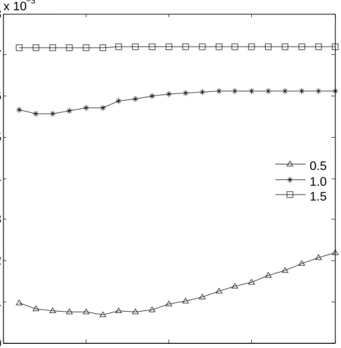
Imposing a majority-rules constraint on the model, it is possible to find the amenity level required for public goods at each location in the city. The measurement of the amenity level is the percent change in housing price per percent change in distance from the public good, i.e., elasticity of price with respect to distance. Because elasticity changes with a household’s distance from the good and rate of decline in the amenity value, results are presented for a representative household and across three levels of the rate of decline. I choose a household 0.01 units from the public good, a distance that qualifies as living ‘close’, and rates of decline equal to 0.5, 1.0, and 1.5. These rates were chosen because they give elasticities consistent with amenity levels found in the
empirical literature for a wide range of public goods (e.g., Luttik 2000, Irwin 2002, Smith, Poulos, and Kim 2002, Jensen and Durham 2003; Vossler et al. 2003, Anderson and West 2006). Figure 2 shows the required amenity level by distance from the city center for the three levels of the rate of decline in amenity value.
<<insert figure 2>>
The lines represent a lower bound on the value placed on the public good. Amenity levels above the lines would receive more than fifty percent of the population’s vote, and the minimum of each line gives the location and absolute lowest amenity level that would receive majority approval. Willingness to pay to be near the public good must be larger the quicker the amenity level declines, shown by the relative placement of lines for each value of . As increases, the distance from the city center matters less, as shown by the relative slopes of the three lines; lower values of produce more variation in the required level of amenity levels than do higher levels of . If the amenity declines slowly (=0.5), the amenity value can be smaller than in cases with higher rates of decline (=1.5) because higher levels of benefits are spread across a greater number of people, but location of the public good matters more with low rates of decline due to the relative increase in importance of taxes and access. The noticeable curvature in the =0.5 scenario highlights an effect that appears in all scenarios – the required amenity level initially falls as distance from the city center increases, showing the effect of taxes on household welfare. Eventually the required amenity level rises as land becomes cheaper and the effect of access dominates.
The results shown in figure 2 can be applied to various types of public goods. A large park, such as what Anderson and West (2006) call special parks (including national, state, or regional parks, arboretums, nature centers, wildlife refuges, and natural areas) is likely to have a high amenity value. If visitors access these parks primarily by car they are likely to be less sensitive to changes in distance than for parks accessed primarily by foot since traveling an extra kilometer by car is quicker for most people than traveling an extra kilometer by foot. Anderson and West (2006) find a 0.03 percent decline in housing prices with a one percent decline in distance from special parks. Examining Figure 2, one must only look for points on any of the lines below 0.03. Provided the amenity does not decline too rapidly, say =1, the model predicts majority support and such a park to be
located near the city center. The minimum required amenity level rises above 0.03 for locations greater than six units from the city center, indicating that a referendum on a special park located further than six units from the city center would not pass. A park with a rate of decline =1 would receive the largest percentage of votes if it were located three units from the city center, since that is the lowest point on the =1 line. If the amenity level declined slower with distance, say =0.5, any location in the city would receive majority support since all points along the =0.5 line are below 0.03. The benefits of a neighborhood park, by definition, do not generally extend beyond the
neighborhood, implying a high . For small neighborhood parks, Anderson and West
(2006) find less than a 0.01 percent decline in housing prices for every one percent decrease in distance from the park. Since 0.01 lies below all the lines depicted in figure 2, the model predicts a referendum on such a park with low and elasticity would fail at any location.
Social Decision Criterion
Next, I compare the results from the voting outcome with a social decision criterion that requires only that aggregate welfare from urban amenities must rise. With identical preferences and willingness to pay, those that benefit from the public good could compensate those that do not benefit for a Pareto improvement. I solve for the minimum amenity level for public goods located at each position in the city that would lead to a net welfare gain across the entire population. This amenity level a(u,v) is shown in figure 3 and must satisfy
q(g p(u,v))1a(u,v) qg1 du dv r(u,v)r
ag 0 (25)The left side of (25) is the sum across all households of the welfare change following the provision of the public good. The equation says total benefits must be larger than total costs, or net benefits must be greater than or equal to zero.
<<insert figure 3>>
The level of amenity required by this criterion is much lower than the level required by majority rules voting, as shown by figure 4. Using the majority rules criterion, the location of the public good dictates the distance z needed for the support of half the population, and thus the amenity level a1 required for the marginal voter to receive positive net benefits. Under the alternative social criterion, the amenity level can be lowered until area A equals area B, so total net benefits are positive. The difference in amenity levels between the two criteria represents a large range of welfare improving
public projects that would never pass under a majority-rules requirement. The difference also represents significant amounts of public resources devoted towards public projects at a given location to win majority support.
<<insert figure 4>>
The slopes of the lines in figures 2 and 3 are of opposite sign. In the majority-rules case, the required amenity level increases with distance from the city center, leading to larger public goods further from downtown. The exact opposite is true when requiring net increases in aggregate utility. The further from the city center, the lower the amenity value must be for net welfare to improve. In this scenario taxes dominate the tax-access tradeoff; whereas in the voting scenario, taxes play a role near the city center, but eventually access is more important. Looking again at figure 4, for locations near the edge of town, z and a1 have to be larger than for locations near the city center to encompass fifty percent of the population, leading to upward-sloping lines for the minimum amenity level required in the voting criterion shown in figure 2. The welfare-improving criterion does not regard the number of households that receive increases in welfare, provided total welfare increases. Since land near the edge of town requires a smaller tax bill yet amenities are distributed to households in equal magnitude regardless of location, area A in figure 4 will be larger for land near the edge of town than for land near the city center for a given amenity level. Lower amenity levels for public goods near the edge of town, therefore, will still bring positive changes in aggregate welfare, producing the downward-sloping lines in figure 3.
Discussion
Parameterizing the model shows the minimum amenity levels required at each location in the city under a majority-rules voting policy and the welfare-improving criterion. Significant differences exist between the two decision criteria, indicating that requiring referenda for amenity decisions is likely to lead to inefficient outcomes. Specifically, many urban amenity votes are likely to fail that would lead to welfare improvements, and any urban amenity decisions that do pass will require amenities larger than needed to achieve the society-wide improvements.
The model was developed for one-parcel-at-a-time referenda, but it would be equally valid for consideration of a continuum of public goods throughout the city. The outcome would look much like that shown in figures 2 and 3. Households would continue to approve public goods until diminishing returns to urban amenities led them to vote against a particular referendum. The cumulative effect of voting would contrast even more with the social decision criterion. The magnitude of the results will depend on the parameterization of the model, though the trends and general directions will stay the same. The values, however, are consistent with U.S. data and give results that match those in the valuation literature (e.g., Luttik 2000; Irwin 2002; Smith et al. 2002; Vossler et al. 2003; Anderson and West 2006).
I mention two caveats. First, households’ location remains fixed in the model before, during, and after deciding whether to vote for a public good location. If the households were allowed to move, land prices and population density would be bid up near the most likely public good locations. Households do not own the land on which they reside; they pay rents to developers. All benefits of the public policy would be
eroded by higher prices, and households would be completely indifferent to urban amenity locations. The utility of households in a closed city model without migration would be higher. The key assumption is, in equilibrium, utilities across households are equal. Else, households would want to move and land price prices would be bid up at more desirable locations.
Second, I do not address the empirical finding of interactions between location and enjoyment of many public goods such as open space (Smith, Poulos, and Kim 2002, Anderson and West 2006; Walsh 2007). Households living in congested areas tend to have stronger preferences for open space. This paper addresses neither this complimentary nor the disutility of congestion. With complementarities between location and public good access, one would expect voting preferences to be stronger downtown than they already are. Since welfare improvements would then be tied to household access, the welfare-improving outcome would look more like the voting outcome, decreasing the efficiency loss associated with voting.
Conclusion
The model developed here is the first to predict the location of public goods in an urban model. Imposing voting rules constrains the monocentric city model and restricts where public goods are likely to occur. Majority rules voting requires higher amenity levels than a welfare-improving criterion, by about an order of magnitude in willingness to pay to be near the good. The effect of distance on the minimum amenity level moves in opposite directions between the two criteria. With majority rules, a densely populated city center makes land near downtown more desirable. With a welfare-improving criterion, net
welfare rises for lower amenity levels for urban amenities near the city edge than for those near the city center.
The analysis uses property taxes to finance public goods, which cause land far from the public good to decline in value because households still have to pay but get little benefit. If households varied by income, wealthier households would locate on the desirable and expensive land near the public good while poorer households would locate far from the public good where land is cheap. This raises a number of gentrification and environmental justice concerns. The challenge to policy makers is to design a mechanism that allows poorer households in a city to live near urban amenities. Unfortunately, that may be a formidable task in a world where desirability of a location implies a higher price for that location.
References
Alonso, W., 1964. Location and Land Use. Harvard University Press, Cambridge.
Anderson, Soren T., West, Sarah E., 2006. Open space, residential property values, and spatial context, Regional Science and Urban Economics 36: 773-789.
Armsworth, Paul R., Gretchen C. Daily, Peter Kareiva, and James N. Sanchirico, 2006. Land market feedbacks can undermine biodiversity conservation, Proceedings of the National Academy of Sciences 103(14): 5403-5408.
Banzhaf, H. Spencer and Randall P. Walsh, 2004. Testing for Environmental Gentrification: Migratory Responses to Changes in Environmental Quality, Paper for the 2004 AERE Workshop. Estes Park, CO.
Calabrese, Stephen, Dennis Epple, Thomas Romer, and Holger Sieg, 2006. Local public good provision: Voting, peer effects, and mobility, Journal of Public Economics 90: 959-981.
Consumer Expenditure Survey, 2006. Table 46, Bureau of Labor Statistics, Department of Labor.
Deacon, Robert and Felix Schlaepfer, 2007. The spatial extent of public good benefits: Evidence from voting on river restoration in Switzerland, University of California - Santa Barbara working paper.
Epple, Dennis, Radu Filimon, and Thomas Romer, 1984. Equilibrium among local jurisdictions: Toward an integrated treatment of voting and residential choice, Journal of Public Economics 24: 281-308.
Epple, Dennis and Glenn J. Platt, 1998. Equilibrium and Local Redistribution in an Urban Economy when Households Differ in both Preferences and Incomes, Journal of Urban Economics 43: 23-51.
Epple, Dennis and Thomas Romer, 1991. Mobility and Redistribution, The Journal of Political Economy 99(4): 828-858.
Geoghegan, J., 2002. The value of open spaces in residential land use, Land Use Policy 19(1): 91-98.
Geoghegan, J., L. Lynch, S. Bucholtz, 2003. Capitalization of open spaces into housing values and the residential property tax revenue impacts of agricultural easement programs, Agricultural and Resource Economic Review 32(1): 33-45.
Heintzleman, Martin, 2008. Measuring the Property-Value Effects of Local Land Use and
Preservation Referenda, Clarkson University Working Paper,
http://papers.ssrn.com/so13/papers.cfm?abstract_id=1314833.
Irwin, E.G., 2002. The effects of open space on residential property values, Land
Economics 78(4): 465-480.
Irwin, E.G., N.E. Bockstael, 2001. The problem of identifying land use spillovers:
measuring the effects of open space on residential property values, American
Journal of Agricultural Economics 83(3): 698-704.
Jensen, Dane and Jared Durham, 2003. The Property Value Effects of the South
Ridgeline Trail, Working paper.
Kotchen, Matthew and Shawn Powers, 2006. Explaining the appearance and success of
voter referenda for open-space conservation, Journal of Environmental
Economics and Management 52(1): 373-390.
Laslier, Jean-Francois and Karine Van der Straeten, 2008. A live experiment on approval
voting, Experimental Economics 11:97-105.
Ledyard, John O. and Thomas R. Palfrey, 2002. The approximation of efficient public
good mechanisms by simple voting schemes, Journal of Public Economics 83:
153-171.
Lipman, Barbara J., 2006. A Heavy Load: The Combined Housing and Transportation
Burdens of Working Families, Center for Housing Policy.
Luttik, Joke, 2000. The value of trees, water and open space as reflected by house prices
Mills, E.S., 1967. An aggregative model of resource allocation in a metropolitan area, American Economic Review 57(2): 197-210.
Muth, R.F., 1969. Cities and housing: the spatial pattern of urban residential land use, The University of Chicago Press, Chicago.
Nechyba, Thomas J. and Randall P.Walsh, 2004. Urban Sprawl, The Journal of Economic Perspectives 18(4): 177-200.
Nelson, Erik, Michinori Uwasu, and Stephen Polasky, 2007. Voting on open space: What explains the appearance and support of municipal-level open space conservation referenda in the United States? Ecological Economics 62(3-4): 580-593.
Sieg, Holger, Smith, V. Kerry, Banzhaf, H. Spencer, Walsh, Randy, 2004. Estimating the General Equilibrium Benefits of Large Changes in Spatially Delineated Public Goods, International Economic Review 45(4): 1047-1077.
Smith, V. Kerry, Christine Poulos, and Hyun Kim, 2002. Treating open space as an urban amenity, Resource and Energy Economics 24: 107-129.
Tiebout, C.M., 1956. A Pure Theory of Local Expenditures, The Journal of Political Economy 64(5).
Vossler, Christian A., Joe Kerkvliet, Stephen Polasky, and Olesya Gainutdinova, 2003. Externally validating contingent valuation: an open-space survey and referendum in Corvallis, Oregon, Journal of Economic Behavior & Organization 51: 262-277. Walsh, Randy, 2007. Endogenous open space amenities in a locational equilibrium,
Wu, JunJie and Andrew Plantinga, 2003. The influence of public open space on urban spatial structure, Journal of Environmental Economics and Managment 46: 288-309.
Wu, JunJie, 2006. Environmental amenities, urban sprawl, and community characteristics, Journal of Environmental Economics and Management 52: 527-547.
a0 Additional amenity of parcel at open space Varies Rate of decline of amenity value with distance from the open space Varies
V Utility level of household at initial equilibrium 2702
Percentage of after-commuting income spent on housing 0.5
Elasticity of utility with respect to open space 0.5
t Annual commuting cost per mile, roundtrip $1000
Y Annual household income $40000
c0 Fixed cost of construction independent of location 0
Ratio of housing value to non-land construction costs 1 1/3
rag Agricultural land rents per acre $1000
(
Figure 1. Percentage of voters that would support public good
The height of the cone represents population located throughout the city.
At any location (u,v) the radius of the circle z is expanded until half the
city's population is included within the circle..
0 5 10 15 20 0 1 2 3 4 5 6 7 8x 10 −3
Distance of Open Space from City Center
% ∆ P / % ∆ z 0.5 1.0 1.5
Figure 2. Required amenity levels for public goods with voting
Required amenity levels, measured percent change in willingness
to pay for a percent change in distance from the public good,
increases with distance from the city center. Amenity levels above
the lines would receive more than fifty percent of the vote.
0 5 10 15 20 0 0.5 1 1.5 2 2.5x 10 −3
Distance of Open Space from City Center
% ∆ P / % ∆ z 0.5 1.0 1.5