Debt Policy and the Rate of Return Premium to Leverage

NBER WORKING PAPER SERIES

DEBT POLICY AND THE RATE OF RETURN PREMIUM TO LEVERAGE

Alex Kane Alan J. Marcus Robert L. McDonald

Working Paper No. 11439

NATIONAL BUREAU OF ECONOMIC RESEARCH 1050 Massachusetts Avenue

Cambridge, MA 02138

August 19814

We have benefitted from the comments of two anonymous referees and seminar participants at Boston University and M.I.T. The research reported here is part of the NBER's research program in Financial Markets and Monetary Economics. Any opinions expressed are those

of the authors and not those of the National Bureau of Economic Research.

NBER Working Paper #1439

August 1984

Debt Policy and the Rate of Return

Premium to Leverage

ABSTRACT

Equilibrium in the market for real assets requires that the price of those assets be bid up to reflect the tax shields they can offer to levered firms. Thus there must be an equality between the market values of real assets and the values of optimally levered firms. The standard measure of the advantage to leverage compares the values of levered and unlevered assets, and can be misleading and difficult to interpret. We show that a meaningful measure of the advantage to debt is the extra rate of return, net of a market premium for bankruptcy risk, earned by a levered firm relative to an otherwise-identical unlevered firm. We construct an option valuation model to calculate such a measure and present extensive simulation results. We use this model to compute optimal debt maturities, show how this approach can be used for capital budgeting, and discuss its implications for the comparison of bankruptcy costs versus tax shields.

Alex Kane Alan J. Marcus Robert L. McDonald Boston University School of Management Boston, Massachusetts 02215

DEBT POLICY AND THE RATE OF RETURN PREMIUM TO LEVERAGE

I. Introduction

Several authors have studied the problem of optimal capital structure by examining the tradeoffs between the tax advantage and potential bankruptcy costs attributable to debt finance. Kraus and Litzenberger (1973) use a time-state-preference model, and Kim (1978) uses a mean-variance model to study optimal debt ratios. Scott (1976) presents an intertemporal model of optimal capital structure in a risk-neutral environment. More recently,

Brennan and Schwartz (1978) and Turnbull (1979) have shown that option-pricing methods can be used to value the levered firm as a function of the value of

the unlevered firm, in the same way that an option is valued as a function of the price of the stock. Bankruptcy costs are easily treated in this

framework. Under some assumptions, the contingent claims model allows for a closed

form solution for the value of the levered firm relative to the value

of its assets. More importantly, the valuation formula requires only easily

interpreted

and estimated parameters. It does not require an estimate of the market price of risk.

Both the Brennan-Schwartz and Turnbull papers, however, use "one-period

models. In effect, they give the value of a firm which is levered only for some fixed interval and which then retires the debt and becomes permanently unlevered.1 A more realistic model would account for the fact that the levered firm, having retired its debt at the end of the first period, would

issue new debt, and so on into the future. The value of the levered firm today would be calculated taking into account the present value of all these future debt issues and all possible future bankruptcy costs.

the option to rebalance its debt ratio every I periods, with T determined

endogenously, and where there are costs to bankruptcy, costs to issuing debt,

and a tax advantage to debt finance.2 We also show how this

approach may be

used to perform capital budgeting calculations. This entails measuring the gains from leverage in a new way.

In addition, our approach takes account of the fact that real asset prices should in equilibrium reflect the value of optimal leverage. Thus, it is misdirected to ask by how much a firm raises its value by taking debt.

Instead, the question is more usefully posed as: by how much does a firm lower its value in being suboptimally levered for a particular period of

time. Intuitively it is clear that the loss in value must depend on how long the firm intends to pursue its particular suboptimal policy. This line of reasoning leads us to argue that the correct metric for the advantage to leverage is the extra rate of return earned in equilibrium by an optimally

levered firm.

The issue of optimal maturity illustrates the use of our measure of the advantage to leverage. As mentioned, Brennan and Schwartz compute the

increase in the value of the levered firm from taking debt, assuming that the firm makes a single debt issue, is levered for T periods, and then becomes permanently unlevered. They show that a firm raises its value more by issuing long-term debt than by issuing short-term debt, which is not surprising since the tax shield accumulates for a longer period of time. As Brennan and

Schwartz note, this comparison has no bearing on the question of optimal maturity.

Our measure of the advantage to leverage, on the other hand, is

essentially an annuity-equivalent of the increase in value computed by Brennan and Schwartz. It is sensible to compare the values of different maturity

-2-policies on a per-period basis, and this is what our measure of the advantage to leverage does.

In Section II we make this argument precise by showing how a contingent claims model of firm valuation allows the calculation of the extra rate of return earned by an optimally levered firm compared to its unlevered

counterpart. This measure of the advantage to leverage is a natural

by-product of the solution procedure, and follows directly from our assumption that unlevered assets are priced so as to reflect the value of leverage. The optimal debt ratio is obtained by choosing debt so as to maximize this rate of return advantage. The solution readily accommodates a multi-period

interpretation,

and thus solves the problem of valuing a firm which

periodically rebalances its debt ratio.

In

Section III we present simulation results which show the rate of return advantage to debt, optimal debt ratios, and the optimal maturities predicted by the model, for a variety of personal tax rates. In the absence of

transactions

costs, we obtain the sensible result that optimal maturity is

zero.

With very small costs of issuing debt, however, the optima' maturity ranges from 5 to 25 years, depending on the corporate tax rate. We find that net of flotation and bankruptcy costs, the tax advantage is generally quite small. We also perform comparative static analysis to show how changes in the standard deviation and bankruptcy costs affect optimal maturities and debt ratios. In Section IV we investigate the implications of the model for capital budgeting. Section V concludes.

II.

The Model

We take as given the value of unlevered assets, which are assumed to evolve according to the diffusion process

-3-(1) dA =

aAdt

+ Adz

where dz is the increment to a Wiener process, a is the instantaneous expected rate of return on A and is the instantaneous standard deviation of the rate of return. A is the market value of the unlevered assets; as such, the

effects of corporate taxation and depreciation rules on the cash flows of the unlevered firm are impounded in a and c,.3 If there is an increase in the

investment tax credit, for example, we would expect the price of unlevered assets to rise.

Now consider an otherwise identical, but levered firm. Suppose that at time 0 the firm issues a zero-coupon bond with face value D, which matures at

time

Denote

the market value of the debt at time 0 as P(D).

The debt affects the value of the firm through two channels. First, it creates the possibility of bankruptcy, with associated costs denoted by B;

these potential costs reduce the current market value of the firm. However, offsetting the bankruptcy cost is a flow of tax shields generated by the tax deductibility of interest payments.

We assume that the geometrically amortized difference between the face value and initial market value of the debt is treated as the tax deduction available from issuing debt, and that there is a full loss-offset provision. At every instant, the increased cash flow due to the tax shield is

where 9

is

the corporate tax rate and i is the internal rate of return on the discount bond, i.e.,

i =

.-ln(D/P)

If invested at the after-tax risk-free rate r(1-o), the tax shield on debt would grow at T to5

(2) TSD = . _[D -

P(D)er

-9)T]

1

- r(l

-4-We assume that the firm is prevented by a bond convenent from paying out dividends before maturity. Therefore, if necessary, TSD is available to satisfy the claims of the bondholders at time T. '1ote that in no-bankruptcy states the value of the levered firm is equal to the value of the unlevered firm, plus the value of the accumulated interest tax deductions.

Offsetting the tax advantage to debt is the fact that debt creates the possibility of bankruptcy. The modelling of bankruptcy costs --

denoted

B

--is

critical in determining the firm's optimal behavior, so we will discuss the alternatives at some length.6 The simplest assumption about bankruptcy cost

is that it is a fixed number, which may or may not depend on the amount of debt issued:

B =

b0 + b10

where b0 and b1 are positive constants. Implicitly it is assumed in this case that there is a full loss-offset: bankruptcy costs are independent of the accumulated interest tax shield, which the firm keeps whether or not bankruptcy occurs. The problem with this assumption is that it provides the firm with an opportunity to benefit at the expense of the government. To see this, consider the strategy of issuing debt with a face value far in excess of the

value of the unlevered firm. The debtholders will expect the firm to

default, and thus the market value of debt at time zero will not increase as

the promised debt repayment increases. With a full loss-offset, however, the

tax

deduction will increase as the stated yield to maturity increases. The firm can thus drive to infinity the value of the interest tax deduction, and if the tax shield grows faster than bankruptcy costs7 the firm maximizes its value

by driving the book value of debt to infinity.

In

practice,

there are two reasons why

this

does not occur. First, there

is

no loss-offset (though there are limited loss carry-forwards), so that the

-5-ability of the firm to use tax deductions is limited by taxable income.8 Second, the IRS in practice disallows the interest deduction if the firm is too highly-levered.9 It is clear that the simple specification of

bankruptcy costs is inadequate.

An alternative, which we follow, is to recognize that firms which go bankrupt typically find the bankruptcy preceded by a period in which taxable income is low and tax deductions cannot be used. A firm which goes bankrupt will therefore lose at least part of its tax shields:

(3) B =

b0 + b1D

+ TS

where TS = ISO + _{TSO, i.e. total tax shields are those generated by debt (TSD)} and from other sources (TSO). This specification treats symmetrically tax shields from debt and from other sources. The other tax shields which should be included are mainly those which do not vary with output, such as

depreciation deductions.'° The time t value of TSO is calculated using the

formul a

(4) TSO =

ri_e)

er(_T -

1]

where 6 is the per period fixed tax deductions from sources other than debt. Including tax shields in bankruptcy costs not only proxies for the absence of a loss offset, but also recognizes that firms with shorter maturity debt have greater flexibility in adjusting tax shields to current income levels.

A. Valuation of the Levered Firm

The

first step in solving for the value of the firm is the specification

of the terminal payments to debt and equity holders at the maturity date of

the debt, 1. These conditions may be written as follows (where the last argument in the functions for security values denote time to maturity):

A + _{ISO > 0}

(4a) P(A, D, 0) = TSD - _B;

0> A +

ISO>

_B

B > A + TSD (4b)

E(A,D,0)A-D+TSD; ATSD>D

0;

AISD <D

(A+TSo;

ATSD>D

(4c) V(A, 0, 0) =

A

+ ISO - _{B; 0 > A} + _{TSD > B}

(o;

B>ATSD

These conditions for debt, P(A,D,0), equity E(A,D,0), and firm value,

V(A,D,O) = P + _{E, involve three relevant regions: (1) A + ISO >}

0,

_{in which}

case the firm remains solvent; (2) 0 > A + _{ISO >}

B,

_{in which case the firm} bankrupts, but debt holders receive partial payment; and (3) B >A + _{TSD, in} which case bankruptcy costs exhaust the entire value of the firm.11 The boundary condition for V at time T (0 time to maturity) states that the firm,

if solvent, receives the interest tax shield plus the value of the assets. These boundary conditions account explicitly for the change in time T values due to issuing debt. Any cash flows which are independent of the debt

-7-decision (such as depreciation tax shields) are already included in A or are included in B, and therefore do not appear explicitly in the boundary

condition. Thus, it is assumed that if the firm issues no debt, depreciation deductions are obtained in all states of nature. If the firm issues debt, however, depreciation deductions are lost in bankrupt states and included in B, as explained above. In non-bankrupt states, depreciation deductions need not be added to the value of the firm, since they are already in A.

Let P(A,D,T-t), E(A,D,T-t) and V(A,D,T-t) represent the market values at time t of debt, equity and firm value respectively, where t denotes calendar

time. If A and V were each priced to earn their opportunity costs of capital, then it could be shown [Merton (1977)] that the values of debt, equity, and the firm would all satisfy the partial differential equation (P.D.E.)

(5)

2A2FAA +

_rAFA +

Ft

-

rF

= 0

where

F represents the market value of any contingent claim on the firm.

Equation (5) is the well-known Black-Scholes equation, and forms the basis for the valuation models in Brennan-Schwartz and Turnbull.

In our case, (5) is an inappropriate description of asset returns because both A and V cannot simultaneously be priced to earn rates of return

sufficient to induce investors to hold them. The levered firm earns cash flows identical to those of the unlevered asset, plus a tax shield. However, in equilibrium, the unlevered asset must sell for the same price as the

optimally levered firm. If it did not, buying the unlevered asset and levering it would constitute an arbitrage opportunity. Because the levered firm and its unlevered asset sell for the same price, no one will hold

urilevered

capi tal as an asset. Put differently,

unlevered capi tal will--due

to the foregone tax shield--suffer a rate of return deficiency, which we denote s. The levered firm will earn an adequate rate of return on new

-8-investments only if it is optimally levered; suboptimal leverage will yield a rate of return below the firm's opportunity cost of capital.

To derive the appropriate modification of (5), we follow Constantinides (1978). Starting with the intertemporal CAP1 of Merton (1973), we may write

(6)

where E() is the expectation operator, and BF is the beta of security F. Ito's lemma can then be used to show (Galai and Masulis, 1976) that

=

A(AFA/F)

so that (6) becomes

AF

—E(-)

r)]

(7) =

r

+

AFA/F

[* r]

*

where

a is the equilibrium required rate of return on a security with the same beta as the underlying asset. The term in square brackets in (7) equals the risk premium on such a security.

From Ito's lemma, we obtain

(8) E(dF) = 1 2 A2 _{FAA + aAF} +

Ft

Equating E(dF) from (7) and (8), we ultimately obtain:

2A2FAA +

(r)AFA

+

Ft

-

rF

= 0

*

where

5

= a

-

a,

_{i.e., the deficiency in the rate of return to unlevered}

capital. The term o plays a role precisely analogous to that of the dividend rate paid by equity in the derivation of the value of an option on a stock paying a continuous dividend (c.f. McDonald and Siegel [1984]). is a "drag" 0n the rate of growth of the value of the underlying asset, in the same way

that dividends are a drag on the growth rate of the stock price.12

This derivation has ignored personal taxes. In this paper we will assume that all debt income (including the return on the risk-free asset) is taxed on accrual at the rate u, and that equity income is untaxed. It is then

straightforward to show by repeating the derivation (with equation (6) holding in after-tax terms) that the P.D.E.s for equity (9') and debt (9'') are

(9')

J2A2FAA +

(r(1-u)

-

)AFA

+

Ft

-

r(1-u)F

= 0

(9'')

2A2FAA +

(ro*)AFA

+

Ft

-

rF

0

where = +

a*u/(1_u)

The boundary conditions for (9') and (9'') are given in equation (4). These conditions together with the P.D.E.s (9) determine the values of debt

and equity. We will allow for the possibility of transaction costs associated with the issuance of the debt, and for simplicity assume that such costs are proportional to the market value of the debt issued.'3 Let k, 0<k<1 denote the fraction of debt lost to flotation costs. The equity holders bear these costs. Then the solutions for debt and equity values at time zero (time to maturity T) are:14

(10) P(A,D,T) =

AeTN(d1)

+

e

T(TsDBd2) +

eTB.TSD+DNd4

-AeTN(d3)

(11)

E(A,D,T)

=

AeTN(d5)

- (D - TSD)e

T(d) -

kP(A,D,T)

(12) V(A,D,T) =

E(A,D,T)

+

P(A,D,T)(1

-

k)

ln(A/(B-TSD)) + _(r

*

+

d1 -

.JT ln(A/(D - TSD)) +

(r

vfT

-

* + 2,2)1

d4 = d3 - VT

d ln(A/(D - TSD)) +

(r(1-u)

- + 5 d6 = _d5 JT

These equations can only be solved implicitly, since the tax shield enters the cumulative normal density, and it is a function of P. Furthermore, is also determined endogenously.

The

existence of

in the fundamental valuation equation results in extra

eT terms multiplying A in the solution. It is easiest to think of e_T

as the initial purchase discount an investor would require in order to

willingly

buy and hold (for a period of duration 1) unlevered capital as an

asset. Note that is an easily interpreted measure of the advantage to

leverage, in that it is an annual rate of return: a flow instead of a stock.

s

represents the tax shield earned over the rebalancing

_{period, less flotation}

costs and expected bankruptcy costs over the same period, expressed as a rate

of return.

The parameter ts may be understood as follows: The buyer of the underlying asset pays a price which incorporates the rents from leverage, but the

underlying asset itself does not earn these rents. As an analogy, if the housing market is competitive, the buyer of a house pays a price which incorporates the value of the interest deduction on the mortgage. The

—11—

where

d1 =

d2 =

homeowner does not earn the extra cash flow associated with this deduction, however, unless the home actually is levered. If the home is not levered, the homeowner earns a below-equilibrium rate of return on the housing purchase. In the same way, the underlying asset by itself earns an expected rate of return which is too low since it does not incorporate the interest tax shield.

The solution to (9) is fully consistent with a multiperiod model in which the firm reoptimizes its debt position at the end of every period. The

novelty in this derivation is that the value of the option to issue new debt

is

fully

incorporated into A, the value of the unlevered assets; we assume

that

competitive bidding ensures that firms will earn no rents on the right to

lever an asset (though rents may be

earned

for other reasons). In receiving A

dollars

at maturity, the firm is receiving the value of an asset, assuming that the next owner pays for the right to lever it optimally. Thus, by construction, the value of the terminal payoff incorporates the value of future leverage.15 This is why the model is consistent with a multiperiod interpretation; all future periods present at best zero NPV opportunities with respect to the leverage decision.

The model of capital structure in Scott (1976) also is explicitly multi-period, with the maturity value of the firm reflecting the value of

future leverage. In this sense, his model is quite similar to ours, and

possesses a recursive structure similar to that in our equation (4). However, Scott does not explicitly consider the relationship between the value of the levered firm and the underlying asset. Instead, he values debt and equity relative to the underlying distribution of cash flows; the equilibrium restriction between the value of unlevered assets and firm value that is central to our model has no counterpart in his.

-12-III. Simulation Results

Equation (12) gives the value of the firm as a function of the value of physical capital, A. In equilibrium, however, we have argued that

V(A,D,T) = _{A at the optimal level of D. To satisfy these conditions we must}

find that value of s which is consistent with the two requirements that _{V0 =}

A0 and that debt policy is chosen optimally, i.e., we solve the problem

Max V(D,T,) subject to V(D*,T*,) =

A.

D,T

This value of _{is precisely the equilibrium tax advantage of debt, net of} transaction costs and a bankruptcy risk premium, expressed as a rate of return. The problem of optimal debt structure is equivalent to that of the

maximization of cs

subject

to the constraint that A0 =

V0. Equations (6)

-(8)

provide only relative prices, so we normalize A = 1. We employ the following algorithm to solve the model:

1. Set A = 1 and choose an initial value for o (denoted as and time to maturity for the debt.

2. Conditional on &,

find

the D which maximizes V.

3. Using this D, find that value of s (denoted as which sets V =

1.

4. If s, then return to 2 using as an updated initial

value for 5.

Repeat

until convergence, i.e., until 60 = cSl. 5. Repeat steps 1 - 4 for a new value of time to maturity for debt.

Search over T, for the time to maturity at which the maximized 6

is

greatest.

At convergence we have the values for 0, 1, and s which are simultaneously consistent with the conditions that debt policy is value maximizing (steps 2 and 5) and V0 =

A0 (step3). Given 0, T, and 6,

the

market value of debt,

and hence the optimal debt to value ratio can be calculated. We used tenth-of-a-year intervals in searching over T.

In addition, we can obtain an explicit measure of the effect of bankruptcy costs on the rate of return advantage earned by the levered firm. If the possibility of bankruptcy could be ruled out, so that N(d) = 1 for all i, then given any particular D, T, and P(A,D,T), the valuation equation (11) would reduce to

s*T rT

(12) 1 = e +

(TSD-k)e

(remembering that A is normalized to 1.0). In this case, (12) can be rearranged to yield

(13)

*

=1ln[1(TSDk)erT

T

The value for *

in

(13) is the gross (of bankruptcy costs) tax advantage to

debt finance. When k=0, this value is comparable to the familiar

Modigliani-Miller (1969) formula for the per-period tax advantage per dollar of debt, which also neglects the market assessment of potential bankruptcy

costs. The difference o - o is then a measure of the extent to which the

possibility of bankruptcy costs (including both direct costs and the riskiness of the tax shield) reduces the rate of return advantage from taking debt. Simulation results, below, indicate that the net and gross tax advantage to debt can differ significantly.

Figures 1 and 2 present simulation results for a set of reasonable parameters: 3xplicit bankruptcy cost (b1) equals 1 percent of the book value of debt; (annual, non-interest deductions) equals .06516; the

-14-personal tax rate ranges from 0 to 46 percent; the real risk-free rate is 2 percent (roughly its historical value); and the annual standard deviation of the price of unlevered assets is .25. These parameters are similar to those chosen by Turnbull (1979). Extensive unreported simulations show that the qualitative properties of the model are not sensitive to the particular parameters chosen.

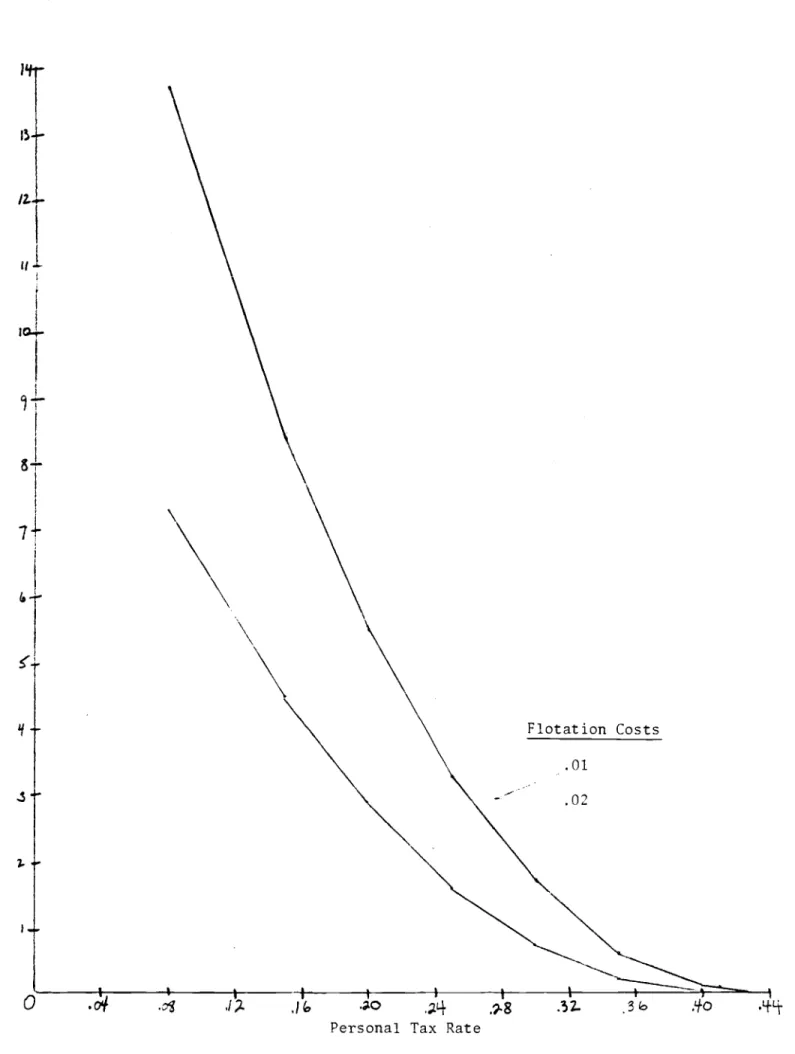
Figure 1 presents the optimal times to maturity for debt issues for

personal tax rates ranging from 1 percent to 44 percent, and for two levels of debt flotation costs: 1.0, and 2.0 percent. As expected, the higher the transactions costs associated with a debt issue, the greater is the optimal maturity

of the debt, since more time is required to amortize the flotation

cost.

In

addition, a high personal tax rate is generally associated with

higher

optimal maturity. This again is due to the fact that at a

lower tax

advantage,

a longer maturity is required to amortize the flotation costs incurred in issuing the debt. At very high personal tax rates, it becomes optimal for the firm to issue no debt because the tax advantage net of

bankruptcy costs is never great enough to offset amortized.transactions costs, whatever the maturity. For a one percent transaction cost, this occurs at a 44 percent personal tax rate, while for two percent transaction cost this occurs at 42 percent.

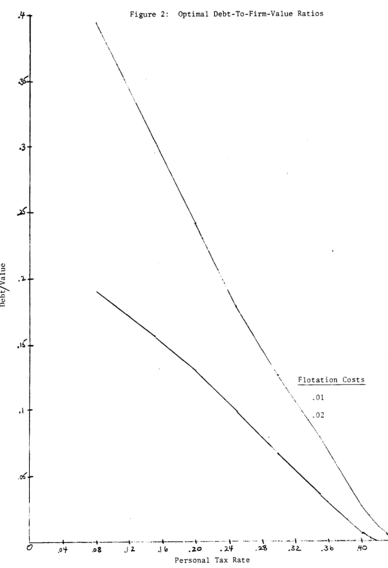
Figure 2 presents optimal debt ratios for the 2 levels of flotation costs, as a function of the tax rate. Optimal debt-to-firm-value ratios increase steadily with the tax advantage to debt. This pattern results from two factors. First, the direct effect of a higher tax advantage is to make debt financing more attractive. Second, the generally lower maturities of debt at higher tax rates (FigUre 1) further induce larger debt ratios because as times to maturity decrease, the bankruptcy probability corresponding to a given debt

-15-ratio also falls. Brennan and Schwartz, Kim, and Turnbull all found optimal debt-to-value ratios of around .5 for corporate tax rates around .5. Thus, the results in Figure 2 for low personal tax rates and one percent transaction cost are comparable to the debt ratios found by other authors.

Figure 3 displays 5,

the

net advantage to debt, as a function of the corporate tax rate. As expected, rises with the corporate tax rate and

falls

with debt flotation cost. Note that the fall in s is riot proportional

to

the difference in amortized

flotation costs. Because optimal maturity

rises

with flotation cost (Figure 1), the amortized flotation cost falls less than proportionally with a fall in the cost, and hence s is not reduced

proportionally to the rise in flotation cost. In addition, of course, the debt-to-value ratio is not held constant in Figure 3.

The tax advantage gross of bankruptcy costs is measured by _{in equation}

(13). Figure 4 plots both s and *

for

a flotation cost of one percent, and

shows that taking into account bankruptcy costs substantially reduces the measured advantage to debt finance.

Figures 5 and 6 perform comparative static analyses for changes in

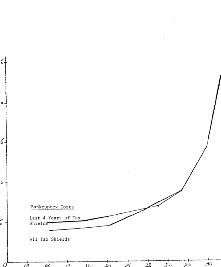
bankruptcy cost and standard deviation. Figure 5A plots optimal maturity for two bankruptcy costs. One case is that where the firm loses all of both the debt and depreciation tax shields when it goes bankrupt.'7 This is the

assumption we make in the previous simulations. The other case assumes that the firm loses only the preceding 4 years

worth of tax shields in the year

when it goes bankrupt. The second case is intended to model the firm which suffers an inability to use tax shields in only the four years preceding

bankruptcy. Obviously when optimal maturity is less than four years, as it is for low personal tax rates, the two cases give the same solution.

Interestingly, however, the two cases also give the same solution for persona'

-16-tax rates above 30 percent. This occurs because the optimal debt ratio is so low at high personal tax rates that bankruptcy costs exceed the face value of

debt.

Footnote 14

shows that the solution for the market value of debt in this

case is independent of bankruptcy costs, so that the higher bankruptcy

cost in the first case is irrelevant to determining the optimal debt ratio.

Figure 5B shows that the increase in bankruptcy costs in the first case

can result in either a higher or lower debt ratio. It is always true that raising bankruptcy cost for a given maturity will lower the optimal debt ratio. In Figure SB the debt ratio is sometimes lower with lower bankruptcy cost because the optimal maturity is greater in those cases (see Figure 5A). The advantage to debt, s, is not depicted but is always greater when

bankruptcy costs are lower. Brennan and Schwartz found a decrease in the optimal debt ratio for an increase in bankruptcy costs, but their results are not directly comparable to ours since they did not allow for changes in

maturity in response to increased bankruptcy costs.

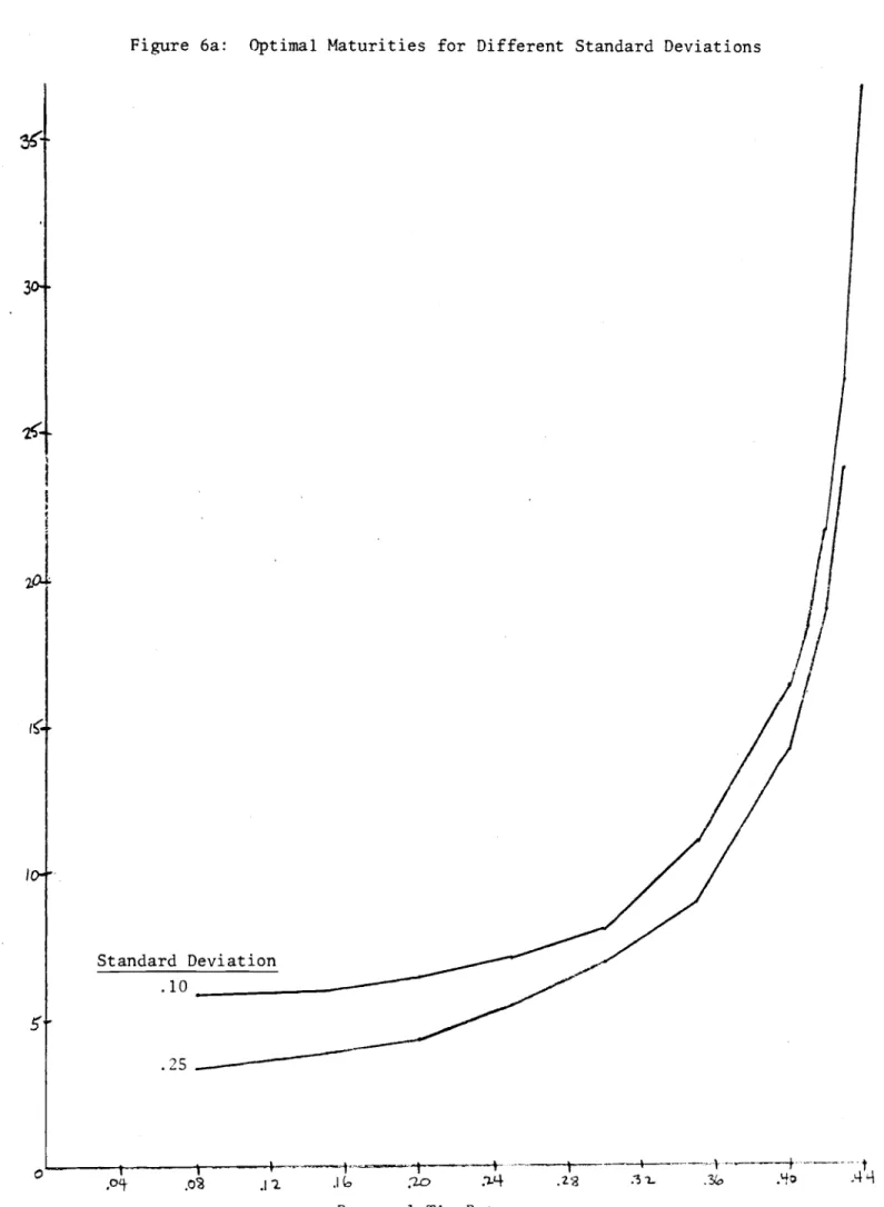
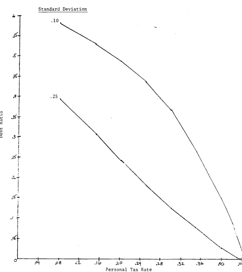
Figures 6A and 6B display the effect on optimal debt ratio and maturity of a decrease in from .25 to .1. The lower standard deviation results in

higher debt ratios, a result also obtained by Brennan and Schwartz. The decrease in standard deviation decreases the chance of bankruptcy for an

initial value of debt and hence increases the debt ratio. Optimal maturity is also

higher with a decrease in

,

reflecting

the fact that with less volatile

asset

returns, the firm rebalances its capital structure less frequently.

IV. Application to Capital Budgeting

A particularly difficult problem in applied finance is capital budgeting

with

taxes and bankruptcy costs. Our model is a relative pricing model, and implies nothing about whether it actually is optimal to undertake a given

-17-project. However, the model does provide a simple technique for dealing with capital budgeting issues in the presence of taxes and bankruptcy costs. The

model implies that it is appropriate to subtract o from the unlevered firm's cost of capital to obtain the appropriate tax- and bankruptcy-adjusted cost of capital.

The

first step in the capital budgeting algorithm is the determination of

a project's (unlevered) beta, and the required hurdle rate if

the project were

operated on an unlevered basis. This is the common starting point for most

modern capital budgeting exercises (Brealey and Myers, 1981, Ch. 18, 19), and

is outside of the concerns of our model. We note, however, that the beta of a

firm can be inferred from the stochastic component of its returns, even if it is

not optimally levered. A

rate-of-return deficiency does not affect

covariance with the market.

Given

the cost of capital for the unlevered project,

one needs only

subtract to obtain the cost of capital for the levered project. The result

is

the appropriate discount rate for the cash flows of the levered firm. This

rate impounds the effect of taxation, bankruptcy and flotation costs; it

is a

generalization

of the tax-adjusted discount rate often presented in introductory finance texts (e.g., Brealey and Myers, pp. 408-12).

The adjustment to the unlevered discount rate is so simple precisely

because s equals the net rate-of-return advantage to leverage. The

appropriate

hurdle rate for the optimally levered project is reduced by

exactly the rate of return advantage provided by leverage.

Further, because cS

can be computed from observable date using the algorithm above, this

adjustment

is a potentially practical way to adjust the discount rate for debt

financing.

-18-V. Conclusion

We have argued that a no-arbitrage condition in the market for real assets will force the price of these assets to be bid up to reflect the tax shields

which they can generate. Therefore, conventional measures of the advantage to

leverage, which attempt to compare the value of levered and unlevered assets, are misleading, since in equilibrium the values must be equal.

However, a well-defined metric for the advantage to debt finance is the difference in rates of return earned by optimally levered and unlevered firms,

net of a return premium to compensate for potential bankruptcy costs. We

derive this measure using a contingent claims framework and present simulation results, which showed that the rate of return advantage as calculated by

considering the tax advantage alone substantially overstates the true

advantage, which is net of a market premium for bankruptcy risk. Simulations

also showed how changes in debt-flotation cost, standard deviation, and

bankruptcy

cost affect optimal maturity and the debt-to-value ratio. We also

demonstrated how to apply our model to the capital budgeting problem.

-19-Footnotes

1 . The model of Brennan and Schwartz can accomodate a single issue of

infinitely-lived debt, and they show that the increase in firm value

approaches a limit as the maturity of the debt increases. This is

obviously a different experiment, however, from allowing an infinite number of debt rollovers (and hence rebalancing of the debt ratio over time) which is the case we will study.

2. Kane, Marcus, and McDonald (1984) use a model similar to this one to

investigate the conditions under which the model is consistent with the

simultaneous existence of levered and unlevered firms. The model in that

paper incorporates personal taxes and a mixed jump-diffusion process on the underlying asset, but does not deal with optimal maturity or study the comparative statics of the model, which are the focus of this paper.

3. This model is partial equilibrium in the sense that take as given the

investment decision. Debt policy is assumed independent of scale, so that

we study optimal debt policy per unit of unlevered assets.

4. Brennan and Schwartz solve the more difficult problem in which the firm issues bonds which pay coupons at discrete intervals. The firm can

bankrupt before T by failing to pay a coupon. However, they still have a

firm which is levered for only a fixed interval .

In

our results below, I

will be set so as to maximize firm value.

5. Both Brennan and Schwartz and Turnbull assume that the tax deduction is

fixed, independent of the yield to maturity on debt, whereas we allow the tax deduction to be based on the actual yield to maturity, as it is in practice.

6.

Turnbull sets bankruptcy costs equal to a fixed fraction of the initial

-20-assets of the firm. Brennan and Schwartz set bankruptcy costs equal to a fraction of the terminal value of the firm. Either of these

specifications is easily incorporated in our framework.

7. Roughly speaking, the condition for this to occur is that the net tax

advantage to debt exceed b1.

8. DeAngelo and Masulis (1980) emphasize the absence of a loss-offset in

determining debt policy.

9. The exact point at which a firm is too highly-levered to qualify for the interest tax deduction is a matter of current policy debate. One proposal

(Commerce Clearing House,1983, 41915) would disallow the interest deduction if the debt-equity ratio exceeded three.

10. By including non-debt tax shields, we are implicitly assuming that these tax shields are always kept if the firm

issues

no debt. This simplifying

assumption captures the fact that issuing debt reduces the marginal value of other tax shields (c.f. DeAngelo and Masulis) but overstates this cost of debt.

11. The boundary conditions (4) and the solutions presented in the text are

valid only if D>B, B>TSD, and D>TSD. To keep the exposition simple we will assume that throughout the text that these conditions hold. Footnote 14 presents solutions for the other cases. The simulations always use the

correct formula for the particular region.

12. Equation (8) is derived assuming that both the levered firm and its

"unlevered"

counterpart make no

dividend

payouts except at dates at which

debt is issued.

Dividends paid just after retirement of one debt issue

and

prior to the next

affect neither the boundary conditions below (up to

the

scale factor A) nor

_equation

(8),

and

therefore would leave our

solution unchanged. If on the

other hand the levered firm pays a flow of

-21-dividends at the dollar rate it(A,t)A at t, then the fundamental P.D.E. becomes

+

Ft

+

FA(ro)A

-

rF

+

A

= 0

and this must be solved subject to the same boundary conditions as (8). It is generally impossible to solve this equation analytically, although a

numerical solution is possible. The same general points would still hold,

and it would turn out, at any rate, that paying dividends would lower the optimal debt-to-value ratio.

13.

The transaction costs result in finite optimal debt maturity. Without

them, if

the

firm chooses T to be infinitessimal, the diffusion process on

A allows close to 100 percent debt financing, yet zero probability of

bankruptcy. Finite maturities are defensible only with flotation costs. 14. The solution presented is valid in the region D>TSD, D>B, and B>TSD. If

these inequalities are violated, different boundary conditions result, and

the solution must be slightly modified. In all of our simulations, the condition D>TSD is satisfied. The solution for equity, equation (10), is always valid as long as D>TSD. The solution for debt, however, depends upon which inequality is violated. If B>D, the solution is

(10')

P(A,D,T) = DeTN(d4),

independent of bankruptcy costs. If B<D but TSD>B,

the solution is

(10")

P(A,D,T) = Ae*T[1N(d3)] + e'T(TSD-B) + eTBTSD+DNd4

where the ds are defined in the text. These solutions are always used

as

appropriate in the simulation analysis.

i.

We assume that the variance rate, 2, and risk free rate, r, are both

-22-constant over time. This implies that the optimal debt ratio and hence o

is the same at each rebalancing point.

16. .065 is the ratio of depreciation deductions to the gross book value of capital in the 1976 IRS Statistics of Income (Corporation Income Tax Returns)

17. The optimal debt ratio sometimes fails to exist with this alternative

defininition of bankruptcy cost. The problem is the same as that

discussed earlier in the text, namely that for long maturities the

increase in the tax shield from issuing additional debt can outweigh the increase in bankruptcy cost, and the optimal debt ratio can be infinite. Essentially, the model assumes that the firm can use all the marginal tax

shields it generates, which is unrealistic. Typically in this case there

is a maturity and debt ratio for which s exhibits a local maximum;

however, at substantially greater maturities and debt ratios begins to rise again, and the timal promised debt repayment then'ecomes unbounded.

Because the unboundedness is the result of assuming a full loss-offset, we treat the local maximum as the correct solution.

References

Brealey, Richard and Stewart Myers. Principles of Corporate Finance, McGraw-Hill, New York, 1981.

Brennan, Michael J. and Edward S. Schwartz. "Corporate Income Taxes, Valuation, and the Problem of Optimal Capital Structure," Journal of

Business 51 (January 1978), 103-114.

ConiTierce Clearing House, Inc. 1984 Federal Tax Course Chicago, 1983.

Constantinides, George M. "Market Kisk Adjustment in Project Valuation,'

Journal of Finance 33 (May 1978), 603-616.

Galai, Dan and R.W. Masulis. "The Option Pricing Model and the Risk Factor

of Stock," Journal of Financial Economics 34 (1976), 53-81.

Kane, Alex, Alan J. Marcus, and Robert L. McDonald. "How Big is the Tax Advantage to Debt "

Journal

of Finance 39 (July 1984), forthcoming.

Kim, E. Han, "A Mean-Variance Theory of Optimal Capital Structure and Corporate Debt Capacity," Journal of Finance 33 (March 1978), 45-63.

Kraus, A. and R. Litzenberger, "A State Preference Theory of Optimal Financial Leverage," Journal of Finance 28 (September 1973), 911-922.

McDonald, Robert and Daniel Siegel. 'Option Pricing when the Underlying Asset Earns a Below-Equilibrium Rate of Return: A Note," Journal of Finance 39,

(March, 1984), 261-265.

Merton, Robert M. "On the Pricing of Contingent Claims and the Modigliani— Miller Theorem," Journal of Financial Economics 5 (November 1977),

241-249.

Miller, Merton. "Debt and Taxes," Journal of Finance 32 (May 1977), 261-27 5.

-24-Modigliani, Franco and Merton H. Miller. "Reply to Hems and Sprenkle,"

Mierican Economic Review 59 (September 1969).

Myers, Stewart C. "Interactions of Corporate Financing and Investment

Decisions --

Implications

for Capital Budgeting," Journal of Finance 29 (March 1974), 1-25.

Scott, •James H. Jr. "A Theory of Optimal Capital Structure," Bell Journal of

Economics 7 (Spring 1976), 33-54.

Turnbull ,

Stuart

t4. "Debt Capacity," Journal of Finance 34 (September 1979),

931-940.

Warner, Jerold. "Bankruptcy Costs: Some Evidence," Journal of Finance 32 (May

1977), 337-347.

-25-—I

C

C.)

:0

5-..

Figure 1: Optimal Time to Maturity of Debt

Flotation Costs 02

Personal Tax Rate

.z.

.3.

...,

.Is

Figure 2: Optimal Debt-To-Firm-Value Ratios

\

Personal Tax Rate

Flotation Costs

.01

.08 2.

.-_ --.---

¾ t -

Figure 3: Net Rate-of-Return Advantage to Debt U 1, 1 Flotation Costs .01 .02 .1

qc

Figure

4: Gross versus Net Advantage to Debt (Flotation Costs =

.01)

Gross Advantage 0 >

0

Advantage 001 .12-. .1 b

Personal Tax Rate

2°-/

-Iz

Figure 5a: Optimal Maturity for Different Bankruptcy Costs

Last 4 Years of Tax

Shiel±

All Tax Shields

0

.ct

.12-

—4——-.-Personal

Tax Rate

Bankruptcy Costs

/

7r3

Personal Tax Rate

Figure Sb: Optimal Debt-to-Firm Value Ratios for Different Bankruptcy Costs

2

Bankruotcy Costs

Last 4 years of tax shields shields

C

30T

1o

Figure 6a: Optimal Maturities for Different Standard Deviations

Standard Deviation

.10

Personal TAx Rate

.4I

C

Figure 6b: Debt-to-Firm-Value Ratios for Different Standard Deviations

Standard Deviation

Personal Tax Rate

'(I, .10 .25 '3

'I

p8

.,2.. •4q