Module 5: Solution of Navier-Stokes Equations for Incompressible Flow Using SIMPLE and MAC Algorithms Lecture 27:

(1)

file:///D|/chitra/nptel_phase2/mechanical/cfd/lecture%2027/27_1.htm[6/20/2012 4:53:40 PM]

Module 5: Solution of Navier-Stokes Equations for Incompressible Flow Using SIMPLE and MAC Algorithms

Lecture 27:

The Lecture deals with: Introduction

Staggered Grid

Semi Implicit Method for Pressure Linked Equations (SIMPLE) x - momentum equation

(2)

Introduction

In Cartesian coordinates, the governing equations for incompressible three-dimensional flows are

(27.1)

(27.2)

(27.3)

(27.4)

In this module no assumption is made about the relative magnitude of the velocity components, consequently the full forms of the Navier-Stokes equations are solved. Methods described in this section will be based, basically, on volume and finite-difference discretization and on the solution of a Poisson equation to determine the pressure. It may be mentioned that these methods use primitive variables and as function of and which are preferable in flow calculations.

(3)

Lecture 27:

Staggered Grid

As it has been seen, the major difficulty encountered during solution of incompressible flow is the non-availability of any obvious equation for the pressure. This difficulty can be resolved in the stream-function-vorticity approach. This approach losses it advantage when three-dimensional flow is computed because of the fact that a single scalar stream-function does not exist in three-dimensional space. A three-dimensional problem demands a primitive-variable approach. Efforts have been made so that two-dimensional as well as three-dimensional problems could be computed following a primitive variable approach without encountering non-physical wiggles in the pressure distribution. As a remedy, it has been suggested to employ a different grid for each of the dependent variables. Such a staggered grid for the dependent variables in a flow field was first used by Harlow and Welch (1965), in their very well known MAC (Maker and Cell) method. Since then, it has been used by many researchers. Specifically, SIMPLE (Semi Implicit method for Pressure Linked equations) procedure of Patankar and Spalding (1972) has become popular. Figure 27.1 shows a two-dimensional staggered grid where dependent variables and with the same indices are staggered to one another. Extension to three-dimensions is straight-forward. The computational domain is divided into a number of cells, which are shown as “main control volume” in Fig. 27.1. The location of the velocity components are at the center of the cell faces to which they are normal. If a uniform grid is used, the locations are exactly at the midway between the grid points. In such cases the pressure difference between the two adjacent the cells is the driving force for the velocity component located at the interface of these cells. The finite-difference approximation is now physically meaningful and the pressure field will accept a reasonable pressure distribution for a correct velocity foeld.

(4)

primitive variables using staggered grid will be discussed in subsequent sections. First we shall discuss the SIMPLE algorithm and then the MAC method will be described.

(5)

Lecture 27:

Semi Implicit Method for Pressure

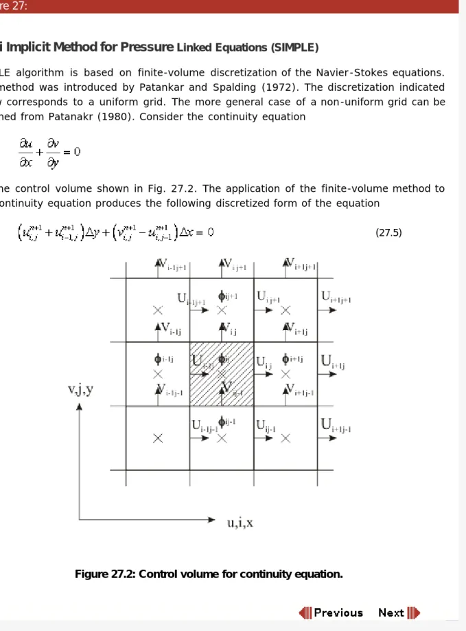
Linked Equations (SIMPLE)

SIMPLE algorithm is based on finite-volume discretization of the Navier-Stokes equations. The method was introduced by Patankar and Spalding (1972). The discretization indicated below corresponds to a uniform grid. The more general case of a non-uniform grid can be obtained from Patanakr (1980). Consider the continuity equation

For the control volume shown in Fig. 27.2. The application of the finite-volume method to the continuity equation produces the following discretized form of the equation

(27.5)

(6)

x – momentum equation

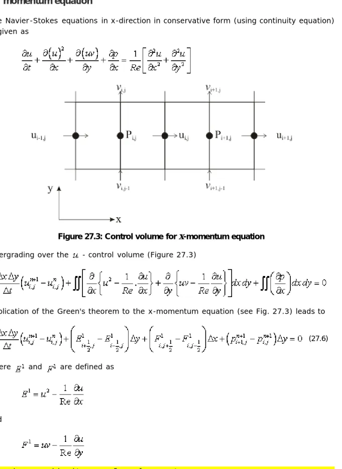
The Navier-Stokes equations in x-direction in conservative form (using continuity equation) is given as

Figure 27.3: Control volume for

x

-momentum equation

Intergrading over the - control volume (Figure 27.3)

Application of the Green's theorem to the x-momentum equation (see Fig. 27.3) leads to (27.6)

where and are defined as

(7)

file:///D|/chitra/nptel_phase2/mechanical/cfd/lecture%2027/27_5.htm[6/20/2012 4:53:41 PM] Thus

(8)

Consequently, eq. (27.6) can be written as

(27.7)

In the above equation, signifies all the convective and diffusive contributions

from the neighboring nodes and their coefficients . The

coefficients and contain grid sizes, and the solution of and at th time level. The term equals In the following sub-section, equation (27.6) has been written term by term so that , and in equation (27.7) can be clearly determined.

Equation (27.6) can be expended as

(9)

Congratulations, you have finished Lecture 27. To view the next lecture select it from the left hand side menu of the page or click the next button.