COPYRIGHT NOTICE
FedUni ResearchOnline
http://researchonline.federation.edu.au
Copyright © 2015 IEEE. Personal use of this material is permitted. Permission from IEEE
must be obtained for all other uses, in any current or future media, including
reprinting/republishing this material for advertising or promotional purposes, creating new
collective works, for resale or redistribution to servers or lists, or reuse of any copyrighted
component of this work in other works.
This is the peer-reviewed version of the following article:
Khorshidi, H., Gunawan, I., Ibrahim, Y.
(2016) Data-driven system
reliability and failure behavior modeling using FMECA.
IEEE Transactions
on Industrial Informatics, 12(3)
, 1253-1260.
Which has been published in final form at:
Abstract—System reliability modelling needs a large amount of
data to estimate the parameters. In addition, reliability estimation is associated with uncertainty. This paper aims to propose a new method to evaluate the failure behavior and reliability of a large system using failure modes, effects and criticality analysis (FMECA). Therefore, qualitative data based on the judgment of experts is used when data is not sufficient. The subjective data of failure modes and causes has been aggregated through the system to develop an overall failure index (OFI). This index not only represents the system reliability behavior but also prioritizes corrective actions based on improvements in system failure. In addition, two optimization models are presented to select optimal actions subject to budget constraint. The associated costs of each corrective action are considered in risk evaluation. Finally, a case study of a manufacturing line is introduced to verify the applicability of the proposed method in industrial environments. The proposed method is compared with conventional FMECA approach. It is shown that the proposed method has a better performance in risk assessment. A sensitivity analysis is provided on the budget amount and the results are discussed.
Index Terms—Failure modes, effects and criticality analysis;
Qualitative data; Uncertainty; Reliability modelling; Universal generating function; Overall failure index; Genetic algorithm.
I. INTRODUCTION
YSTEM evaluation is important to provide a systematic view for engineers in order to identify the problems and improve them. Reliability has been increasingly considered in system analysis to reduce system failure [1]. Many researchers have done investigation on developing system reliability models to assess and optimize system behavior and safety via components’ working probability and performance [2-7]. The exact value of the probability is not easily accessible [8, 9]. To estimate these parameters by statistical models, large amount
Copyright (c) xxxx IEEE. Personal use of this material is permitted. However, permission to use this material for any other purposes must be obtained from the IEEE by sending a request to [email protected].
H. A. Khorshidi is with the School of Applied Sciences and Engineering, Faculty of Science, Monash University, Victoria, Australia (corresponding author to provide phone: +61-4-75025021; fax: +61-3-51226738; e-mail: [email protected]).
I. Gunawan is with the School of Engineering and Information Technology, Federation University Australia, Churchill, VIC 3842, Australia (e-mail: [email protected]).
M. Y. Ibrahim is with the School of Engineering and Information Technology, Federation University Australia, Churchill, VIC 3842, Australia (e-mail: [email protected]).
of data is needed. In addition to this, the estimation is associated with uncertainty [10]. Therefore, subjective estimates of parameters which are based on the judgment of experts and engineers could be useful in the situation with the lack of sufficient data [11].
Failure modes and effects analysis (FMEA) is a qualitative risk assessment method which makes possible using linguistic expressions when historical data and statistics are not available [12]. It aims to identify potential failure modes, investigate their effect on the system, specify the causes, prioritize them, and allocate corrective actions to the crucial ones. A failure mode is a situation in which an asset or a component cannot work properly [13]. In order to ranking failure modes, each possible failure mode is valued by three parameters as severity (S), occurrence likelihood (O), and detection difficulty (D) to obtain a risk priority number (RPN). These parameters are rated among 1 to 10 to show how the failure mode is severely influenced the system, how often it happens, and how much it is detectable before having consequences, respectively. The RPN value is calculated through multiplication of the parameters which is RPN=S×O×D. The company can consider a strategy to implement improvement actions based on the highest RPN value, or a predefined threshold to remove or mitigate cause of failures [14]. Failure modes, effects and criticality analysis (FMECA) is an extended version of FMEA which is combined with criticality analysis (CA) procedure [15].
FMECA is a bottom-up approach which consists of a breakdown structure for reliability examination of the final item of the system based on the failure causes [12, 16]. System definition and modelling is usually used to understand the system’s operation to determine failure modes and their cause and effects [15]. Sharma et al. [17] utilized fault tree and petrinet models to determine the relationship between failure modes and subsystems. Boolean representation method (BRM) is integrated with FMECA in [18] to model cause and effect relationships. A prioritization method is proposed for failures in system FMEA to consider relations between components by decision making trial and evaluation laboratory technique (DEMATEL) [19]. Chen [20] used a hierarchical FMEA system structure to analyze a company from bottom (cause of failure) to top (system). These system models try to find the RPN value of each failure mode to rank them through the system so that the system reliability will be improved by applying corrective actions on critical failure causes. However in the current study, we are going to find a
Data-driven system reliability and failure
behavior modelling using FMECA
Hadi A. Khorshidi, Indra Gunawan, and M. Yousef Ibrahim, Senior Member, IEEE
failure index for the whole system based on FMECA by reliability block diagram (RBD) and universal generating function (UGF). This model can contain the data of failure modes, components, and subsystems and the interaction among them through a large scale system. Also, this approach is useful for decision makers to find the priority of each improvement action based on their effect on the whole system. One of the main criticisms of the RPN method is that the associated cost is not considered in analysis. Some studies have been done to point out cost in FMEA. The cost caused by failure is used as severity, occurrence and detection parameters are expressed by probabilities to establish the expected cost by [21]. Bevilacqua et al. [22] employed maintenance cost in calculation of priority number in FMECA. A Life Cost-Based FMEA is introduced in [23] for comparing and selecting design alternatives. Carmignani [12] considered the cost of corrective actions in applying improvement for failure modes. A fuzzy cost-based FMEA is integrated with grey rational analysis (GRA) and profitability theory to prioritize service failures [24]. In this paper, the associated uncertainty with reliability evaluation is quantified by subjective estimates of FMECA approach. Therefore, the failure behavior of the system can be modelled when there is lack of sufficient data. A systematic approach is proposed to estimate system reliability and failure using qualitative data. As a result, the proposed approach can assess the potential corrective actions of the industrial system. Furthermore, two optimization models are developed to find the optimal combination of actions via considering corrective actions’ cost.
The rest of paper is organized as follows. The second section presents the proposed method through some subsections such as systematic view, system behavior modelling, prioritization, and optimal selection. The third section illustrates the proposed methods via a case study of a
manufacturing line. The concluding remarks are mentioned in the last section.
II. PROPOSED METHOD
In this section, the proposed method is presented for system reliability modelling via FMECA, mathematical formulation and optimization model in the following subsections. At first, a systematic view is introduced for failure modes in an FMECA approach. Then, the failure behavior of the system is assessed by UGF approach to reach a failure index. After that, the system failure index is utilized to rank the corrective actions in terms of providing reduction in system risk. Finally, an optimization model is developed to select corrective actions economically.
A. Systematic view
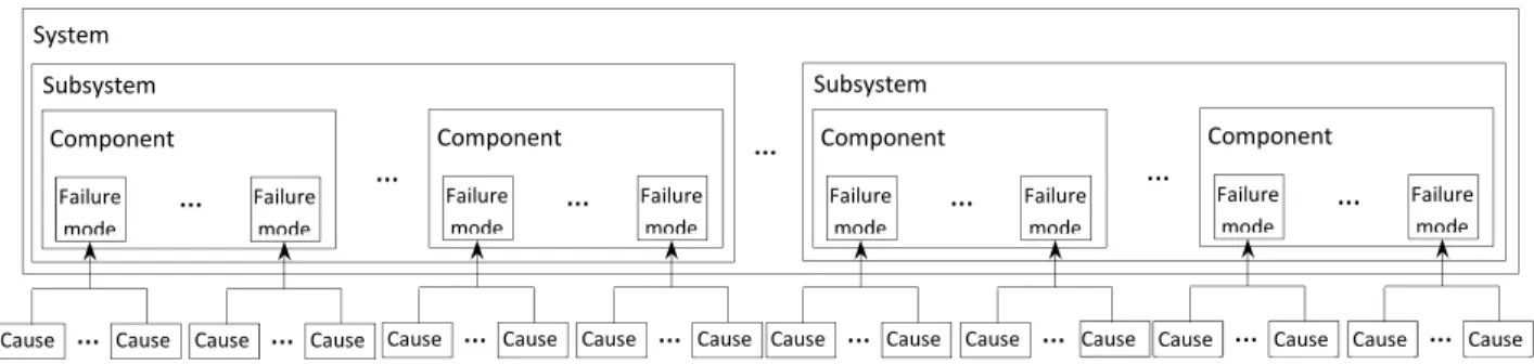
A qualitative analysis of the system is carried out using the integration of hierarchical algorithm and block diagram to provide a system sketch based on FMECA which is shown in Figure 1. At the bottom of the framework, there are failures and their causes. Each failure mode may consist of some failure causes. Therefore, the failures are analyzed based on the severity of the effect of the failure mode on the next higher level or the system, the occurrence probability of the failure cause, and the detection capability for each failure cause. In fact, occurrence and detection parameters are obtained from causes, and severity is for failure mode [25, 26]. The higher level shows that each component includes some failure modes which lead the component to fail. Based on the system configuration, components and subsystems can form the system RBD.
Since a component will fail when a failure mode occurs, each component is a series system in which failure modes are elements. Therefore, different levels (states) of failure would be imposed to each component based on the seriousness of the
Cause
…
Cause Failure mode Cause…
Cause Failure mode…
Component Cause…
Cause Failure mode Cause…
Cause Failure mode…
Component…
Subsystem Cause…
Cause Failure mode Cause…
Cause Failure mode…
Component Cause…
Cause Failure mode Cause…
Cause Failure mode…
Component…
Subsystem…
SystemFigure 1. System structure
Hydraulic oil tank
No# Rate Severity
1 0.443 4
2 0.103 3
3 0.059 3
4 0.395 4
Auxiliary
No# Rate Severity
1 0.284 3 2 0.011 3 3 0.085 3 4 0.566 4 5 0.011 3 6 0.043 2 Control
No# Rate Severity
1 0.015 2 2 0.310 4 3 0.365 3 4 0.155 1 5 0.155 1 Protection
No# Rate Severity
1 0.132 3 2 0.066 1 3 0.530 4 4 0.046 1 5 0.066 1 6 0.066 1 7 0.066 1 8 0.028 1 Hydraulic servo transmission
No# Rate Severity
1 0.094 1 2 0.522 4 3 0.013 1 4 0.311 1 5 0.026 1 6 0.026 3 7 0.008 1 Figure 2. HHTS configuration
happened failure mode. If several failure modes occur at the same time, the maximum of the severity the occurred failure modes represents the failure level of the component at that time. This concept is used in the next section to find the overall failure index (OFI).
B. System behavior modelling
In this section, the FMECA information of the failure modes is aggregated through the system using the UGF approach. Therefore, the uncertainties are propagated across the whole system [27]. To make an illustration, an example is adapted from [18] which is exhibited in Figure 2. The example is a hydraulic hoisting transmission system (HHTS) of a marine crane with five subsystems in which failure modes are defined. Each failure mode is analyzed by occurrence rate and severity. In some work on FMECA (or FMEA), the detection parameter does not take into account. Kmenta et al. [28] suggest eliminating detection in priority evaluation of failure modes. In [29], the importance weight of detection has been found one-third of severity and half of occurrence through pair wise comparison of analytic hierarchy process (AHP). Also, occurrence level and severity classification are used in the application of FMECA for product traceability in food industry [30]. The critical processes are selected for implementing statistical process control (SPC) via occurrence likelihood and severity of their failure modes [31]. In fuzzy risk analysis, two factors of severity and failure probability are usually used to evaluate the risk of components [32].
In UGF, the probability distribution of a variable (X) is discretely represented via a u-function (Eq. 1) in which p is the probability that the variable is in state j, x is its corresponding value, and k shows the number of different states of the variable. The u-function presents a polynomial structure of a probability distribution. This transformation provides an opportunity to use the properties of polynomial expressions in order to find the probability distribution of a function of variables. It also facilitates to model a system with multi-level components [33, 34].
uz = ∑ p ∙ z
(1)
According to this, we aim to create a u-function for each failure mode. Each failure mode is considered as a binary phenomenon which consists of two possible reliability levels. These levels are failure and functioning states. Therefore, each failure mode follows the binomial (Bernoulli) distribution. Where, occurrence rate represents the probability that a failure mode occurs with specified severity degree. According to this statistical property, the probability distribution of each failure mode can be presented by u-function as Eq. 2.
u z = ∑ Or ∙ z (2)
where u z is the u-function of failure mode number i in subsystem h, Or and S are respectively the occurrence rate and severity of the failure mode in state j. Since there are just two states as 0 stands for failure and 1 stands for working state (no failure), Or = 1 − Or. Also, severity of the state with no failure (S) is zero. Consequently, the u-function of the failure mode number 1 in subsystem 1 ( uz ) is
demonstrated as 0.443×z4+0.557×z0.
Based on the failure modes’ u-functions, the behavior distribution of the higher levels such as components, subsystems, and system can be obtained. In this regard, all possible combinations should be considered to generate the u-function of the higher level item via the ⊗ operator. For the example, u-function of each subsystem can be computed as Eq. 3.
uz =⊗!"#uz, u%z, … , u'z( (3) where uz is the u-function of subsystem h, n* is the number of failures in the subsystem, and ⊗!" denotes the maximum severity of the occurred failures in each combination is considered. A Matlab programming is developed to acquire the probability distribution of severity levels of subsystems. The results are exhibited in Table 1.
TABLE 1.
PROBABILITY DISTRIBUTION OF SUBSYSTEMS
As can be seen, the binary-state failures lead to multi-state subsystems. The u-function of subsystems can be obtained based on the probability distribution outcomes. For example, the u-function of subsystem 1 ( uz ) is as 0.663×z4+0.0525×z3+0.2844×z0. Similarly, the u-function of the system is figured based on the subsystems’ u-functions through considering all possible combinations of severity levels of subsystems. Since the subsystems of the example are connected as a series system, the u-function of the whole system is obtained as Eq. 4.
Uz =⊗!",uz, u%z, … , u'z- (4)
where Uz is the u-function of the system, and n is the number subsystems. The severity levels of the system which are calculated through Matlab software are shown in Table 2. These levels and the corresponding probabilities are reached by analyzing 960 different combinations (3×4×5×4×4).
TABLE 2.
PROBABILITY DISTRIBUTION OF THE SYSTEM
Severity level 0 1 2 3 4
probability 0.0019 0.0043 0.0004 0.0161 0.9773
According to Table 2, the u-function of the system is as 0.9773×z4+0.0161×z3+0.0004×z2+0.0043×z1+0.0019×z0. An expected value for each u-function can be extracted using the first derivative at z equal to 1. As a result, a derivation is to be done on the system’s u-function to find the expected value of the system in terms of failure as OFI (Eq. 5).
OFI =010Uz at z = 1 (5) Subsequently, the OFI for the example is computed which is 3.9627. The u-function represents how the system tends to be failed, and the OFI gives a scale to measure this failure
Subsystem 1 Severity level 0 3 4
probability 0.2844 0.0525 0.663
Subsystem 2 Severity level 0 2 3 4
probability 0.2662 0.012 0.1559 0.566
Subsystem 3 Severity level 0 1 2 3 4
probability 0.3082 0.1234 0.0066 0.2518 0.31
Subsystem 4 Severity level 0 1 3 4
probability 0.2879 0.1201 0.062 0.53
Subsystem 5 Severity level 0 1 3 4
behavior.
C. Prioritization
This section is allocated to use the OFI in ranking corrective actions based on their improvement on the whole system failure behavior. Corrective actions are usually applied on to decrease the occurring rate or increase the detectability of the causes. Therefore, a corrective action controls the related cause in terms of occurrence or detection. Then, it would lead to mitigate the risk of each failure mode. Successively, it effects on the items in the higher levels as component, subsystem, and system according to Figure 1. As a result, the OFI would be reduced in the response of implementing the corrective action. This reduction can be used as criteria to prioritize the corrective actions as Eq. 6.
∆OFI"= OFI67889:;− OFI" (6) where OFI" is the estimated OFI for the time the corrective action a is applied on the corresponded failure cause, and
∆OFI" measures the reduction that is carried out on the current situation of the system (OFI67889:;) by action a. The higher the
∆OFI, the higher the priority of corrective action to apply. Consequently, the corrective actions which have more impact on the improvement on the system behavior can be nominated. An example is developed for illustration. Given an action is applied on failure 4 in subsystem 2 (F<=) which improves the occurrence rate from 0.566 to 0.2. It changes the OFI to 3.9312, so that the ∆OFI of the action is 0.0315. Also, the occurrence rate of the failure F>< is improved by another action from 0.53 to 0.2. As a result, the OFI is promoted to 3.9365 which the reduction of 0.0262 has been obtained. According to these results, the action for F<= is in higher priority for implementation because of the higher improvement on system failure. In addition, it can be seen that two failures with same severity level and almost the same improvement in occurrence rate can have different impacts on
the system. It shows the existence of different importance weight for the failures. In conventional RPN method, failure modes are ranked based on their risk and corrective actions are allocated to the more critical modes. However, the effectiveness of the allocated actions is not considered. In the proposed method, the most effective actions are selected to reduce the system failure.
D. Optimal selection
Due to the limited budget, all corrective actions cannot be allocated to all failure causes. Therefore, a balance should be provided between actions’ costs and their equivalent improvement. As a result, an algorithm has been developed to select optimal corrective actions using an optimization model. The algorithm aims to maximize the resulted reduction in OFI by corrective actions in terms of the budget constraint. The linear mathematical formulation of the optimization model is as Eq. 7.
Max ∑@ ∆OFI"∙ x" "
∑@ C"∙ x"
" ≤ B (7)
where x" is a Boolean variable that is 1 if action a is applied otherwise is 0, N is the number of failure causes which is equal to ∑:*n*, C" is the cost associated with the action, and
B is the available budget.
In the abovementioned model, the effect of several corrective actions on OFI is assumed to be linear. However, there is a nonlinear relationship between OFI reduction and number of applied actions. For example, if two mentioned actions in previous section apply concurrently, the reduction in OFI is 0.0798; while it is not the summation of the individual
∆OFI (0.0315 and 0.0262). As a result, the optimization model is changed to a modelling with nonlinear objective function and still a linear constraint as Eq. 8.
Max ∆OFIX ∑@ C"∙ x" " ≤ B (8) Inserting in cells Cellular welding Lid insertion Pole welding Punched shells storage Punching Plates, separators, and shells Final storage Packaging Plate batches storage Plate welding Punched shells Coupling test Welding test Plates & separator s Shells
where X is a vector of Boolean variable as X = x, x=, … , x@. Solving this model will give how many actions and which of them are optimal to apply.
To sum up, the steps in the proposed method to reach the final decision are brought as follows:
• Develop block diagram and hierarchical algorithm to break down the system into failure modes and causes
• Assess the failure modes by FMECA parameters
• Allocate corrective actions to the causes, and estimate their improved parameters
• Aggregate the failure modes based on system structure to reach OFI
• Calculate the OFI for each corrective action based on the estimated parameters
• Rank corrective actions in terms of the difference they make on OFI (∆OFI)
• Select the optimal set of corrective actions subject to budget constraint
III. CASE STUDY
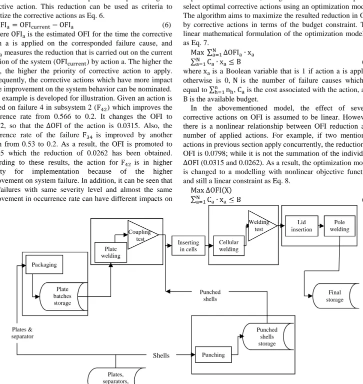
The proposed method is implemented in a case study to validate its applicability. In this case study, three parameters of the RPN method have been employed. The considered case is a manufacturing line of car battery factory. The processes of the manufacturing line are shown in Figure 3. After this line, the battery shells go to another manufacturing line for filling electrolyte inside.
In fact, a Process FMEA (PFMEA) has been done on the manufacturing processes. The manufacturing line consists of six processes such as 1) packaging, 2) plate welding, 3) punching, 4) inserting in cell, 5) cellular welding, 6) housing. Each process is considered as a block (component), therefore, the block diagram of the manufacturing line is drawn as Figure 4.
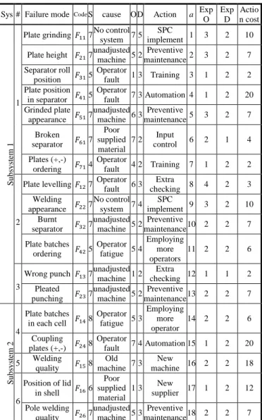
Failure modes of each process have been identified. A root cause analysis (RCA) is done to find the cause of failure occurrence, and suggest a corrective action for each failure cause. Also, failure modes are evaluated based on severity, occurrence, and detection parameters. All parameters are individually rated from 1 to 10 based on the standard tables of FMECA [35]. The historical data of each failure is investigated to measure the occurrence rate. For occurrence, numbers 10 and 1 denote that the possibility of failure incidence is extremely high and nearly impossible respectively. However, the severity and detection parameters have been rated using experts’ judgements. For severity, if the failure mode has hazardous consequence for the whole system is rated as 10, and if there is no effect is rated as 1. For detection, number 10 shows that the control system does not detect the potential cause of the failure before occurrence, and
number 1 shows the cause is easily detectable. The result of FMECA application is presented in Table 3. It should be mentioned that Exp O and Exp D are the expected values of occurrence and detection after applying the corrective actions respectively, and action cost denotes the associated cost of the corrective action.
TABLE 3.
FMECA FOR THE MANUFACTURING LINE
In this case, we have three parameters of FMECA in the scale of 1-10. Therefore, some modifications should be taken in order to developing u-function. First of all, the occurrence rate in an interval of [0,1] is needed to use in UGF approach. To reach this goal, the frequency factor which is proposed in [12] as the percentage of occurring a failure cause can be employed as the occurrence rate. However in our case, since we tend to keep FMECA’s properties, the occurrence rate is defined through dividing occurrence value (O) over 10 (i.e. if the occurrence value is 5, the occurrence rate would be 0.5). Secondly, the detection value should be involved in u-function structure. According to these modifications, the u-function of each failure mode is constructed as Eq. 9.
u z = ∑ Or ∙ z ×F
(9)
where D is the detection of failure mode i in state j which it is zero in state of no failure. Accordingly, the calculation of OFI
Sys # Failure mode Code S cause O D Action a Exp
O Exp D Actio n cost S u b sy st em 1 1
Plate grinding H 7 No control system 7 5
SPC
implement 1 3 2 10 Plate height H= 7 unadjusted machine 5 2 Preventive
maintenance 2 3 2 7 Separator roll position H> 5 Operator fault 1 3 Training 3 1 2 2 Plate position in separator H< 5 Operator fault 7 3 Automation 4 1 2 20 Grinded plate appearance HI 7 unadjusted machine 6 3 Preventive maintenance 5 3 2 7 Broken separator HJ 7 Poor supplied material 7 2 control Input 6 2 1 4 Plates (+,-) ordering HK 4 Operator fault 4 2 Training 7 1 2 2 2
Plate levelling H= 7 Operator fault 6 3 Extra checking 8 4 2 3 Welding appearance H== 7 No control system 7 4 SPC implement 9 3 2 10 Burnt separator H>= 7 unadjusted machine 5 2 Preventive maintenance 10 2 2 7 Plate batches ordering H<= 5 Operator fatigue 5 4 Employing more operators 11 2 2 6 3
Wrong punch H> 7 unadjusted machine 1 2 Extra
checking 12 1 1 2 Pleated punching H=> 7 unadjusted machine 5 2 Preventive maintenance 13 2 2 7 S u b sy st em 2 4 Plate batches in each cell H< 8 Operator fatigue 5 3 Employing more operator 14 2 2 6 Coupling plates (+,-) H=< 8 Operator fault 7 4 Automation 15 1 2 20 5 Welding quality HI 8 Old machine 7 3 New machine 16 2 2 18 6 Position of lid in shell HJ 6 Poor supplied material 1 3 New supplier 17 1 2 12 Pole welding quality H=J 7 unadjusted machine 5 3 Preventive maintenance 18 2 2 7 3 1 2 4 5 6 Subsystem 1 Subsystem 2
Figure 4. The case study RBD
I II
is modified in Eq. 10 for considering three parameters in their original scale. In fact, the OFI could be equivalent with the RPN value which lies in the interval of 1 to 1000. Therefore, the RPN has been extended so that each component, subsystem, and system can have an RPN value.
OFI = 10 × 010Uz|1 (10) As a result, the u-function has been developed for each failure mode of the case based on Eq. 9. Hence, the OFI value is computed for each process as is presented in Table 4. As can be seen, the computed OFI value for process 5 is equal with the RPN value of FI (8×7×3) due to having just one failure mode.
TABLE 4.
OFI OF EACH PROCESS
Process 1 2 3 4 5 6
OFI 299.95 250 77 260 168 114
To reach the OFI value of the whole system, in subsystem 1 branch I, there are two components (1 and 2) which are connected in a series structure. After that, two branches of subsystem 1 are working in parallel. However, they do not have the properties of parallel systems in RBDs because the next block needs the output of both branches. In other word, two branches are connected in a 2-out-of-2 system structure. A k-out-of-n system works if and only if at least k components work, whereas a parallel system works while at least one component works. An n-out-of-n system is a series system, and a 1-out-of-n system is a parallel system [36, 37]. Consequently, two branches behave as a series system. In subsystem 2, three components are connected in as a series structure. By considering the mentioned system structure, the OFI value of the manufacturing line has been obtained. The OFI for subsystem 1, subsystem 2, and system are 322.17, 290.33, and 336.19 respectively.
After finding the system’s OFI value, ∆OFI of each corrective action based on its improvement on occurrence and detection parameters can be calculated. Therefore, ∆OFI is useful for ranking the corrective actions in order to implementation. Table 5 shows the obtained ∆OFIs and their ranking. Also, a comparison is provided with the conventional RPN method in Table 5.
TABLE 5.
PRIORITIZATION RESULTS
Action ΔOFIO Ranking ∆OFI Failure mode RPN Ranking RPN
1 32.23 1 H 245 1 2 0.00006 15 H= 70 12 3 0.00005 16 H> 15 17 4 0.0012 10 H< 105 8 5 0.017 6 HI 126 5 6 0.0003 12 HJ 98 11 7 0.00003 17 HK 32 15 8 0.0169 7 H= 126 5 9 2.83 3 H== 196 3 10 0.00009 13 H>= 70 12 11 0.0081 9 H<= 100 10 12 0.00001 18 H> 14 18 13 0.00009 13 H=> 70 12 14 0.1321 5 H< 120 7 15 11.23 2 H=< 224 2 16 0.31 4 HI 168 4 17 0.0005 11 HJ 18 16 18 0.0113 8 H=J 105 8
The actions have been prioritized in terms of their impact on mitigating OFI of the system. The associated actions of the high risk failure modes with higher RPN values (i.e. actions 1, 15, 9, and 16) reach the higher places in ranking because they improve occurring rate and detection of the high risk failures. However, ∆OFI presents different ranking order for other actions in comparison with the RPN. For example, action 14 stands on the fifth level while its equivalent failure mode (F<) was in the 7th place by RPN. The main difference of these methods is that RPN ranks the failure modes, but ∆OFI prioritizes the corrective actions. The ∆OFI method finds which corrective action should be applied in terms of their impact on improving the failure behavior of the whole system. Therefore, the proposed ∆OFI not only evaluates the importance of the failure mode, but also checks whether the allocated actions are appropriate to reduce system failure. Also, one of the shortcomings of the conventional RPN is that it generates many duplicate numbers for ranking the failures [19, 26, 35, 38], ∆OFI has the lower duplication rate due to having more parameters involved. There are just two corrective actions with the same ∆OFI value which are in the 13th level, however, some repetitive values for RPN can be found such as 70, 105, and 126. Therefore, RPN cannot rank seven different failure modes properly.
As can be seen in Table 3, the corrective actions are associated with the cost. Particularly, the higher the actions’ priority, the higher the cost is assigned. Therefore, a budget limitation (B) as 74 has been considered through optimization models. The simplex linear programming model which is introduced in Eq. 7 is constructed by the obtained ∆OFI values and cost information. It has been solved by the Excel solver, and the results of the optimal selection are presented in Table 6.
TABLE 6.
OPTIMAL RESULTS OF LINEAR MODEL
Actions
∆OFI Cost
P P= P> P< PI PJ PK PQ PRPPP=P>P<PIPJPKPQ
1 0 0 0 1 0 0 1 1 0 0 0 0 1 1 1 0 0 142.36 74
In the optimal solution, 7 corrective actions have been selected and the entire budget is consumed. For the non-linear objective function which is introduced in Eq. 8, a Matlab programming has been developed. Also, a penalty function approach has been considered to deal with the budget constraint. Penalty functions turn constrained problems into unconstrained problem by penalizing infeasible solutions [39]. In our work, the penalty-based method proposed in [40] is used to define the feasible solutions. Finally, the model is solved by genetic algorithm (GA) which the results are shown in Table 7.
TABLE 7.
OPTIMAL RESULTS OF NON-LINEAR MODEL
Actions
∆OFI Cost
P P= P> P< PI PJ PK PQ PRPPP=P>P<PIPJPKPQ
1 0 0 0 1 0 0 1 1 0 0 0 0 1 1 1 0 0 142.36 74
In the optimal solution, the same corrective actions have been selected. The optimization model works to find which actions and how many should be taken. As can be seen, both models reach to similar optimal selection.
Discussion
We would like to investigate scenarios with different budget levels. Therefore, the models have been solved through a decrease in budget (B=37) and an increase in budget (B=112) which Table 8 shows the results.
TABLE 8.
SENSITIVITY ANALYSIS
Model Budget Actions ∆OFI Cost
PP=P>P<PIPJPKPQPRPPP=P>P<PIPJPKPQ
Linear 37 1 0 0 0 1 0 0 0 0 0 0 0 0 0 1 0 0 0 69.85 37
112 1 0 0 1 1 1 0 1 1 0 1 0 0 1 1 1 0 1 184.75 111
Nonlinear 37 1 0 0 0 0 0 0 1 0 0 0 0 0 1 1 0 0 0 71.13 36
112 1 0 1 1 1 0 1 1 1 0 1 0 0 1 1 1 0 1 184.84 111
As it was expected by growing the budget the number of selected actions and the ∆OFI has been increased and vice versa. To compare the two models, the nonlinear model finds better optimal selection in budget limitation of 37 through the same number of actions with lower cost. In budget constraint of 112, the nonlinear model reaches to the higher objective function with more corrective actions. As a result, the nonlinear model works stronger than the linear model to find the optimal selection. However, the linear model could be more practical due to its simplicity and exactness.
In addition, the situation that a failure mode has an occurrence value of 10 is investigated. Since the occurrence rate is obtained via dividing on 10, the occurrence rate of this failure is equal to 1. It causes that the behavior of the related component be shown as a failed component. For example, if the occurrence value of F becomes 10, the proposed method finds that there is not the state of ‘no failure’ for packaging process. It is reasonable because the failure is almost inevitable when the occurrence value is 10. Therefore, this situation is crucial, and the occurrence rate must be reduced with the highest priority. It is recommended to use parallel structure for the component or sub-process to diminish the occurrence rate.
IV. CONCLUSION
In this study, a new method is proposed to model the system failure behavior using qualitative data. The proposed method helps practitioners to perform system evaluation in terms of risk and reliability when enough data is not accessible. The practitioners can utilize experts’ judgements using FMECA to investigate system reliability via the proposed method which makes a simpler procedure. The UGF approach propagates the obtained qualitative data from failure mode levels to system levels. The three main goals of this study are (i) integration uncertainty in system reliability evaluation using linguistic expression when there is not sufficient statistical data, (ii) prioritization the corrective action in terms of their impact on the whole system failure, (iii) considering actions’ cost in order to select the optimal combination of corrective actions for implementation. Therefore, an index has been developed named OFI to represent the failure behavior of the system using FMECA’s parameters. Furthermore, two optimization models are proposed to find the optimal selection of corrective actions subject to the budget constraint. Finally, a real case study on the manufacturing line of the car battery factory is
presented. The proposed method is applied on the mentioned case step by step. The performance of the proposed method is compared with the conventional RPN method, and the results are discussed. Two optimization models have been compared based on the obtained results. Also, a crucial situation of having a failure mode with occurrence value of 10 is introduced, and it is suggested to improve it with the highest priority based on the proposed method. For further research, fuzzy logic can be integrated in the proposed method.
REFERENCES
[1] Afonso, L. D., Mariani, V. C. & Dos Santos Coelho, L. Modified imperialist competitive algorithm based on attraction and repulsion concepts for reliability-redundancy optimization. Expert Systems with
Applications 40 (9), (2013) 3794-3802.
[2] Calderaro, V., Lattarulo, V., Piccolo, A. & Siano, P. Optimal switch placement by alliance algorithm for improving microgrids reliability.
IEEE Transactions on Industrial Informatics 8 (4), (2012) 925-934.
[3] Garg, H., Rani, M., Sharma, S. P. & Vishwakarma, Y. Bi-objective optimization of the reliability-redundancy allocation problem for series-parallel system. Journal of Manufacturing Systems 33 (3), (2014) 335-347.
[4] Hamadani, A. Z. & Khorshidi, H. A. System reliability optimization using time value of money. International Journal of Advanced
Manufacturing Technology 66 (1-4), (2013) 97-106.
[5] Khorshidi, H. A., Gunawan, I. & Ibrahim, M. Y. On Reliability Evaluation of Multistate Weighted k-out-of-n System Using Present Value. Engineering Economist 60 (1), (2015) 22-39.
[6] Willig, A. Redundancy concepts to increase transmission reliability in wireless industrial LANs. IEEE Transactions on Industrial Informatics 1 (3), (2005) 173-182.
[7] Zhao, B., Aydin, H. & Zhu, D. On maximizing reliability of real-time embedded applications under hard energy constraint. IEEE Transactions
on Industrial Informatics 6 (3), (2010) 316-328.
[8] Garg, H., Rani, M. & Sharma, S. P. An approach for analyzing the reliability of industrial systems using soft-computing based technique.
Expert Systems with Applications 41 (2), (2014) 489-501.
[9] Verma, M. & Kumar, A. A novel general approach to evaluating the reliability of gas turbine system. Engineering Applications of Artificial
Intelligence 28 (0), (2014) 13-21.
[10] Strangas, E. G., Aviyente, S., Neely, J. D. & Zaidi, S. S. H. The effect of failure prognosis and mitigation on the reliability of permanent-magnet AC motor drives. IEEE Transactions on Industrial Electronics 60 (8), (2013) 3519-3528.
[11] Braaksma, A. J. J., Meesters, A. J., Klingenberg, W. & Hicks, C. A quantitative method for Failure Mode and Effects Analysis.
International Journal of Production Research 50 (23), (2012)
6904-6917.
[12] Carmignani, G. An integrated structural framework to cost-based FMECA: The priority-cost FMECA. Reliability Engineering and System
Safety 94 (4), (2009) 861-871.
[13] Selim, H., Yunusoglu, M. G. & Yılmaz Balaman, Ş. A Dynamic Maintenance Planning Framework Based on Fuzzy TOPSIS and FMEA: Application in an International Food Company. Quality and Reliability
Engineering International (In press) (2015)
[14] Jamshidi, A., Rahimi, S. A., Ait-Kadi, D. & Ruiz, A. A comprehensive fuzzy risk-based maintenance framework for prioritization of medical devices. Applied Soft Computing 32 (2015) 322-334.
[15] Bouti, A. & Kadi, D. A. A STATE-OF-THE-ART REVIEW OF FMEA/FMECA. International Journal of Reliability, Quality and Safety
Engineering 1 (4), (1994) 515-543.
[16] Zhou, A., Yu, D. & Zhang, W. A research on intelligent fault diagnosis of wind turbines based on ontology and FMECA. Advanced Engineering
Informatics 29 (1), (2015) 115-125.
[17] Sharma, R. K., Kumar, D. & Kumar, P. Fuzzy modeling of system behavior for risk and reliability analysis. International Journal of
Systems Science 39 (6), (2008) 563-581.
[18] Wang, J., Ruxton, T. & Labrie, C. R. Design for safety of engineering systems with multiple failure state variables. Reliability Engineering &
[19] Seyed-Hosseini, S. M., Safaei, N. & Asgharpour, M. J. Reprioritization of failures in a system failure mode and effects analysis by decision making trial and evaluation laboratory technique. Reliability
Engineering & System Safety 91 (8), (2006) 872-881.
[20] Chen, C. C. A developed autonomous preventive maintenance programme using RCA and FMEA. International Journal of Production
Research 51 (18), (2013) 5404-5412.
[21] Gilchrist, W. Modelling Failure Modes and Effects Analysis.
International Journal of Quality & Reliability Management 10 (5),
(1993) 16-23.
[22] Bevilacqua, M., Braglia, M. & Gabbrielli, R. Monte Carlo simulation approach for a modified FMECA in a power plant. Quality and
Reliability Engineering International 16 (4), (2000) 313-324.
[23] Rhee, S. J. & Ishii, K. Using cost based FMEA to enhance reliability and serviceability. Advanced Engineering Informatics 17 (3-4), (2003) 179-188.
[24] Abbasgholizadeh Rahimi, S., Jamshidi, A., Ait-Kadi, D. & Ruiz, A. Using fuzzy cost-based FMEA, GRA and profitability theory for minimizing failures at a healthcare diagnosis service. Quality and
Reliability Engineering International (In press) (2013)
[25] De Souza, R. V. B. & Carpinetti, L. C. R. A FMEA-based approach to prioritize waste reduction in lean implementation. International Journal
of Quality and Reliability Management 31 (4), (2014) 346-366.
[26] Sankar, N. R. & Prabhu, B. S. Modified approach for prioritization of failures in a system failure mode and effects analysis. International
Journal of Quality and Reliability Management 18 (3), (2001) 324-335.
[27] Huimin, L., Monti, A. & Ponci, F. A Fuzzy-Based Sensor Validation Strategy for AC Motor Drives. IEEE Transactions on Industrial
Informatics 8 (4), (2012) 839-848.
[28] Kmenta, S., Fitch, P. & Ishii, K. Advanced failure modes and effects analysis of complex processes.in Proc. ASME Design Engineering
Technical Conferences (Las Vegas, USA, 1999).
[29] Braglia, M. MAFMA: Multi-attribute failure mode analysis.
International Journal of Quality and Reliability Management 17 (9),
(2000) 1017-1033.
[30] Bertolini, M., Bevilacqua, M. & Massini, R. FMECA approach to product traceability in the food industry. Food Control 17 (2), (2006) 137-145.
[31] Khorshidi, H. A., Gunawan, I. & Esmaeilzadeh, F. Implementation of SPC with FMEA in less-developed industries with a case study in car battery manufactory. International Journal of Quality and Innovation 2 (2), (2013) 148-157.
[32] Khorshidi, H., Gunawan, I. & Nikfalazar, S. Application of Fuzzy Risk Analysis for Selecting Critical Processes in Implementation of SPC with a Case Study. Group Decision and Negotiation (In press) (2015) [33] Levitin, G., The Universal Generating Function in reliability analysis
and optimization, Springer-Verlag: London, 2005).
[34] Lisnianski, A., Frenkel, I. & Ding, Y., Multi-state system reliability
analysis and optimization for engineers and industrial managers,
Springer-Verlag: London, 2010).
[35] Chang, K. H., Chang, Y. C. & Lai, P. T. Applying the concept of exponential approach to enhance the assessment capability of FMEA.
Journal of Intelligent Manufacturing 25 (6), (2013) 1413-1427.
[36] Huang, J., Zuo, M. J. & Wu, Y. Generalized multi-state k-out-of-n:G systems IEEE Transactions on Reliability 49 (1), (2000) 105-111. [37] Khorshidi, H. A., Gunawan, I. & Ibrahim, M. Y. Investigation on system
reliability optimization based on classification of criteria.in Proc. IEEE
International Conference on Industrial Technology (ICIT) (South
Africa, 2013).
[38] Chang, D. S. & Sun, K. L. P. Applying DEA to enhance assessment capability of FMEA. International Journal of Quality and Reliability
Management 26 (6), (2009) 629-643.
[39] Smith, J. C. & Coit, D. W., Penalty Functions. In: BACK, T., FOGEL, D. B. & MICHALEWICZ, Z. (eds.) Handbook of Evolutionary
Computation. (Bristol: Oxford University Press, 1997).
[40] Chen, T. C. IAs based approach for reliability redundancy allocation problems. Applied Mathematics and Computation 182 (2), (2006) 1556-1567.
Hadi Akbarzade Khorshidi is a PhD student in the
School of Applied Sciences and Engineering at Monash University, Australia. He received his master in Industrial Engineering from Isfahan University of Technology, Iran, in 2010. Also, he received his B.Sc. in Rail Transportation Engineering from Iran University of
Science and Technology, Iran, in 2008. His research interests are in Reliability Engineering, Optimization, Quality Technology, Decision Making, and System Dynamics. He has published his research papers in many peer-reviewed journals and conferences.
Indra Gunawan is a Senior Lecturer and Coordinator
of Postgraduate Programs in Maintenance and Reliability Engineering in the School of Engineering and Information Technology at Federation University, Gippsland Campus, Australia. He completed his Ph.D. degree in Industrial Engineering from Northeastern University, USA. His main areas of research are maintenance and reliability engineering, project management, application of operations research, operations management, applied statistics, probability modeling, and engineering systems design. His work has appeared in many peer-reviewed journals and conference proceedings.
M. Yousef Ibrahim received his PhD in 1993 from
University of Wollongong. He is a faculty member of Federation University Australia (FUA). Before FUA, he joined Monash University where he established the Graduate Certificate in Reliability Engineering by distance education. In 1997, he established the Master Degree in Maintenance and Reliability Engineering by also by distance education. He initiated and developed the Monash's degree in Mechatronics which is currently offered at both Clayton and Kuala-Lumpur campuses. He is also the founder of the Mechatronics program currently offered at Federation University Australia. Professor Ibrahim is currently on his fifth consecutive term as member on a Ministerial Advisory Council to the Minister for Innovation and Small Business of the State Government of Victoria, Australia. He has research interests in Life Cycle Costs, Reliability Engineering, Mechatronics and industrial automation.