Algorithm and intelligent tutoring system design for ladder logic programming

(1)

ALGORITHM AND INTELLIGENT TUTORING SYSTEM DESIGN FOR LADDER LOGIC PROGRAMMING

A Thesis by

YUAN-TENG CHENG

Submitted to the Office of Graduate Studies of Texas A&M University

in partial fulfillment of the requirements for the degree of MASTER OF SCIENCE

August 2007

(2)

LADDER LOGIC PROGRAMMING

A Thesis by

YUAN-TENG CHENG

Submitted to the Office of Graduate Studies of Texas A&M University

in partial fulfillment of the requirements for the degree of MASTER OF SCIENCE

Approved by:

Co-Chairs of Committee, Sheng-Jen "Tony" Hsieh

Dezhen Song

Committee Member, Sing-Hoi Sze Head of Department, Valerie E. Taylor

August 2007

(3)

iii

ABSTRACT

Algorithm and Intelligent Tutoring System Design for Ladder Logic Programming. (August 2007)

Yuan-Teng Cheng, B.S., National Tsing Hua University Co-Chairs of Advisory Committee: Dr. Sheng-Jen "Tony" Hsieh

Dr. Dezhen Song

With the help of the internet, teaching is not constrained in the traditional classroom pedagogy; the instructors can put the course material on the website and allow the students go on to the course webpage as an alternative way to learn the domain knowledge. The problem here is how to design a web-based system that is intelligent and adaptive enough to teach the students domain knowledge in Programmable Logic Controller (PLC).

In my research, I proposed a system architecture which combines the pre-test, cased-based reasoning (i.e., heuristic functions), tutorials and tests of the domain concepts, and post-test (i.e., including pre-exam and post-exam) to customize students’ needs according to their knowledge levels and help them learn the PLC concepts effectively.

I have developed an intelligent tutoring system which is mainly based on the feedback and learning preference of the users’ questionnaires. It includes many pictures, colorful diagrams, and interesting animations (i.e., switch control of the user’s rung configuration) to attract the users’ attention.

(4)

From the model simulation results, a knowledge proficiency effect occurs on problem-solving time. If the students are more knowledgeable about PLC concepts, they will take less time to complete problems than those who are not as proficient.

Additionally, from the system experiments, the results indicate that the learning algorithm in this system is robust enough to pinpoint the most accurate error pattern (i.e., almost 90 percent accuracy of mapping to the most similar error pattern), and the adaptive system will have a higher accuracy of discerning the error patterns which are close to the answers of the PLC problems when the databases have more built-in error patterns.

The participant evaluation indicates that after using this system, the users will learn how to solve the problems and have a much better performance than before. After evaluating the tutoring system, we also ask the participants to submit the survey (feedback), which will be taken into serious consideration in our future work.

(5)

v

DEDICATION

(6)

ACKNOWLEDGMENTS

I would like to thank my committee chair, Dr. Hsieh, co-chair, Dr. Song, and my committee member, Dr. Sze, for their guidance and support throughout the course of this research.

Thanks also to my friends and colleagues and the department faculty and staff for making my time at Texas A&M University a great experience.

(7)

vii

NOMENCLATURE

BN Bayesian Network

CBR Case-Based Reasoning

CTU Count Up

CU Count Up Enable Bit DAG Directed Acyclic Graph DBN Dynamic Bayesian Networks

DN Done Bit

EN Enable Bit

ITS Intelligent Tutoring System JPD Joint Probability Distribution

KB Knowledge Base

NO Normally Open switch NC Normally Closed switch

NCSR Normally Closed Spring Return switch NOSR Normally Open Spring Return switch

OOP Object-Oriented Programming

OTE Output Energize

PLC Programmable Logic Controller RES Count Reset Bit

SM Student Model SVM Support Vector Machine

(8)

TM Tutor Model

TON Timer On-Delay

TOF Timer Off-Delay

TT Timing Bit

UI User Interface

VPLC Virtual Programmable Logic Controller XIC Examine if Closed

(9)

ix TABLE OF CONTENTS Page ABSTRACT ………..………. … iii DEDICATION ………... v ACKNOWLEDGMENTS.……….. vi NOMENCLATURE…….……….. vii TABLE OF CONTENTS ……….. ix LIST OF FIGURES ……….……….. xi

LIST OF TABLES ….…….……….. xiii

CHAPTER I INTRODUCTION ………. 1

1.1 Motives ……….. 1

1.2 Research Objectives……….. 2

1.3 Format of this Investigation………... 2

II LITERATURE REVIEW………. 3

2.1 Introduction………. 3

2.2 Curriculum Sequencing………... 5

2.3 Adaptive Collaboration Support……….. 6

2.4 Case-Based Reasoning………. 6

2.5 Ontology Extraction………. 6

2.6 Semantic Web……….. 7

2.7 Dynamic Bayesian Networks……….. 7

2.8 Classification and Clustering……….. 10

2.9 Genetic Algorithms……….. 11 2.10 Summary……… 11 III METHODOLOGY………... 14 3.1 Introduction……….. 14 3.2 Assumptions……….. ……….. ……… 14

(10)

CHAPTER Page

3.3 Learning Algorithm………. 15

3.4 Proposed System………. 21

IV SYSTEM IMPLEMENTATION……... 32

4.1 System Programming and Environment Setting………. 32

4.2 Introduction to Programming Logic Diagrams………….. ……… 33

4.3 User Configuration Mapping………….. ……….. ……… 37

4.4 System Layout Snapshot. ……….. ……… 40

V EVALUATION AND RESULTS……….. 42

5.1 Introduction……….. 42

5.2 Simulation Experiments and Results……….. 42

5.3 Summary………. 64

VI SUMMARY AND CONCLUSIONS………... 65

6.1 Summary………. 65

6.2 Conclusion and Future Work……….. 66

REFERENCES……….. 68

APPENDIX……… 72

(11)

xi

LIST OF FIGURES

FIGURE Page

2.1Primitive framework of Intelligent Tutoring System………. 4

2.2Intelligent Tutoring System framework with an adaptive model…………... 5

2.3An illustrative simple Bayesian Network……… 8

2.4Dynamic Bayesian Network changes with time………. 9

3.1 Learning algorithm of Intelligent Tutoring System………. 16

3.2 Heuristic functions………... 17

3.3 An example of rung configurations………. 19

3.4 Proposed system architecture……….. 22

3.5 Student learning preference distribution………. 23

3.6 Directed acyclic graph, where white circles means concepts and yellow rectangles represent 10 Flash PLC problems, respectively.……… 27

3.7 System flowchart………. 29

4.1 Programming tools and program execution flow……….... 32

4.2 An example of the rung configuration………. 36

4.3 System working area setting of one of the hidden rungs………. 37

4.4 Before coordinate recalculation of one of the hidden rungs……… 38

4.5 After coordinate recalculation of one of the hidden rungs……….. 38

4.6 Path enable/disable determination of one of the hidden rungs……… 39

4.7 System snapshot of the experiment window……… 41

5.1 Mapping accuracy based on different number of heuristic functions…... 52

(12)

FIGURE Page 5.3 User performance before and after the system experiment………. 57 5.4 State diagram of the change of problems for a professional student (i.e.,

80% chance pass for each problem at the first time)………... 59 5.5 Student experiment time of all 10 problems………..………. 60 5.6 Triangle distribution of Problem1……….……….. 62 5.7 System simulation time based on students who have different knowledge proficiency……….. 63

(13)

xiii

LIST OF TABLES

TABLE Page

2.1 Comparative study of different approaches………. 12

3.1 Calculation of heuristic functions H(n)………20

3.2 Predefined student knowledge level and concepts classification……… 25

4.1 Detail explanation of PLC software components……… 34

4.2 Detail explanation of PLC hardware components………... 35

5.1 Error patterns of Problem1……….…... 44

5.2 Matching patterns and accuracy measurements of Problem1…..……….….. 48

5.3 Use different number of heuristic functions to find the average mapping accuracy………... 51

5.4 Use HF5 to measure the average accuracy based on different databases…… 54

5.5 User test score before and after the system experiment……….….. 57

(14)

CHAPTER I INTRODUCTION

1.1 Motives

Although traditional classroom teaching is undoubtedly the best way for students to learn, limited lecture time prevents teachers from using the preferred one-on-one instructional format. With the widespread use of computers in society, almost everyone can access the internet to search and learn. This allows instructors to put class materials on websites, and helps students strengthen or clarify their concepts, especially through such web-based systems, Intelligent Tutoring Systems (ITSs).

There are many ITSs spread around the world which aim to teach students domain knowledge in some specific applications. However, most of these tutoring applications lack interactive ability (i.e., the rules for generating the teaching path are embedded and unchanged overtime). An intelligent system should have the adaptive ability to learn and become increasing robust as time goes on.

________________

(15)

2

1.2 Research Objectives

From recent research of intelligent tutoring systems (Woolf & Murray, 1994; Eliot & Woolf, 1995; Beck, Stern, & Woolf, 1997; Beck & Woolf, 1998; Cassin, Eliot, Lesser, Rawlins, & Woolf, 2004; Woolf, 2004), we know that machine learning as well as optimized and customized pedagogical teaching for students is the direction in which next-generation intelligent systems development is headed. Here, based on the ongoing direction, we want to develop a web-based tutoring system with machine learning algorithms which will result in the generation of efficient and personalized pedagogical strategies, and put our experimental emphasis on the Programmable Logic Controller (PLC) application.

1.3 Format of this Investigation

This chapter describes the motives and research objectives of this study. In Chapter II, we review eight research areas which relate to the solution of this problem: Curriculum Sequencing, Adaptive Collaboration Support, Case-Based Reasoning, Ontology Extraction, Semantic Web, Dynamic Bayesian Networks, Classification and Clustering, and Genetic Algorithms. Chapter III describes the algorithm to solve this problem and also gives an illustrative example, and also mentions about the system architecture and execution processes. In Chapter IV, the system implementation is explained and the demonstration of logic diagram control is shown in the snapshot of the system interface. Chapter V describes the participant evaluation and results. Finally, the summary and conclusion of this research are presented in Chapter VI.

(16)

CHAPTER II LITERATURE REVIEW

2.1 Introduction

From the survey paper (Petrushin, 1995; Tsiriga & Virvou, 2004; Su, Chen, & Yih, 2006), we know that the goal of intelligent tutoring systems is to help students gain an in-depth knowledge of certain kinds of domains. Students learn and test their knowledge through refined guiding processes/tutorials and evaluation questions of ITSs. The systems generate the concept questions from the knowledge base in which the students show interest, organize the questions by using the Tutor Model (TM), and then present them to the students through the User Interface (UI). The whole retrieval and generation cycle is the core idea of intelligent tutoring systems.

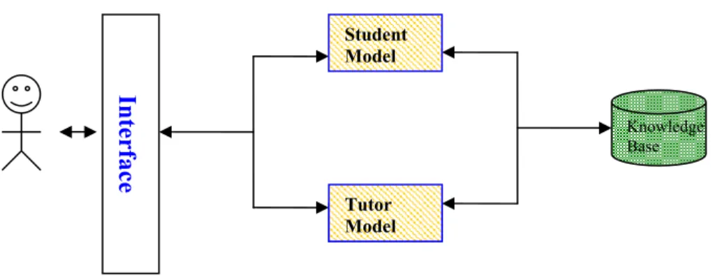
In order to enhance students’ learning, many teachers and researchers devote much time to the development of web-based tutoring systems that allow instructors to incorporate their class slides and handouts into it. ITSs are composed of User Interface (UI), Student Model (SM), Tutoring Model (TM) and Knowledge Base (KB). The relations between these models are shown in Figure 2.1.

(17)

4

Figure 2.1 Primitive framework of Intelligent Tutoring System.

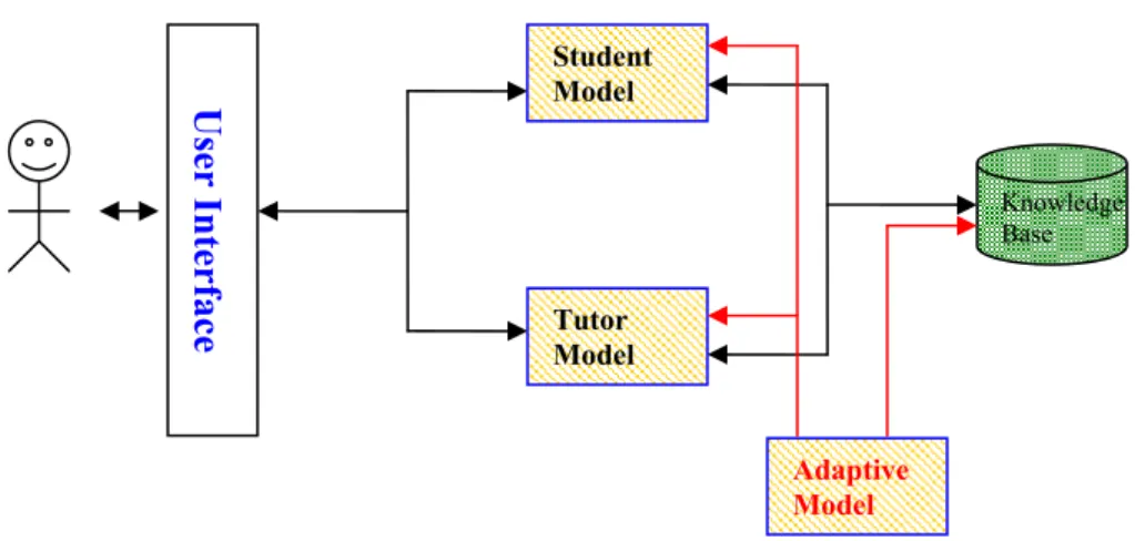
However, this framework is static. Every student using this system experiences the same learning steps and same recommended instructions every time. This system cannot provide a learning model that is well-suited to the specific needs of individual students. Hence, in recent years, almost all research publications in this area focus on how to develop adaptive models (i.e., the Student Model or even the Tutoring Model will learn and update their database), and personalized models (i.e., generating the most suitable Student Model for specific students), for the intelligent tutoring system (see Figure 2.2). There are many trivial details in these publications; thus in the following subsections, we summarize the main methods prevalent in this research area, put them into different categories according to their main differences, and briefly describe their contributions. Student Model Knowledge Base Interface Model Tutor Model

(18)

Figure 2.2 Intelligent Tutoring System framework with an adaptive model.

2.2 Curriculum Sequencing

Curriculum Sequencing (Beck & Woolf, 1998; Brusilovsky, 1999) is the latest topic researchers have used for finding the optimal path of a specific problem for the current user. From Figure 2.1, we can see that the tutoring sequence is constructed by the Tutor Model first, and then presented on the User Interface to guide the student through the problem solving. However, traditional static ITSs cannot dynamically generate the optimal learning path for the current user, and this sometimes frustrates the user when he/she wants to re-experience this same topic. In order to raise the user’s satisfaction, one could also use the Curriculum Sequencing method. When the user initially logs in to this system, he/she must finish a pre-test (i.e., some simple questions presented to the user to identify the user’s knowledge in this domain). Then Curriculum Sequencing tries to find the best learning path for this user from the current knowledge base.

Student Model Tutor Model User Interface Knowledge Base Adaptive Model

(19)

6

2.3 Adaptive Collaboration Support

Collaboration Support (Brusilovsky, 1999; Tsiriga & Virvou, 2004; Zhou, Wu, & Zhang, 2005) means that once the ITS system is unable to give the current user the correct solution, the user can search for the solution among the remote partners. After the user receives the solution, the Student Model and Tutor Model update the database to include the exceptional or alternative solution. This approach is also called Adaptive Collaboration Support.

2.4 Case-Based Reasoning

The goal of Case-Based Reasoning (CBR) (Mitrovic & Djordjevic-Kajan, 1995; Sindi, 2005) is to find the most similar existing case for the current student, adapt this case to meet the student's situation, and then update the case models in the database. The main problem here is how to discern the most similar case for the current user. To find this case, one may use approximation algorithms such as the k-nearest neighbor algorithm (Tsiriga & Virvou, 2004), which aims to find the sum of the minimum square differences among the current user and the existent user models, and the rule-based classification algorithms (Akhras, 2005; Granic & Glavinic, 2005), which use comprehensive built-in rules to identify the user queries or corresponding reactions.

2.5 Ontology Extraction

Ontology Extraction (Petrushin, 1995; Cassin, Eliot, Lesser, Rawlins, & Woolf, 2004; Devedzic, 2003; Bredeche, Shi, & Zucker, 2006) is a two-phase method used to

(20)

build an abstraction tree for different ITS applications. The first phase is to extract the topics or core skeleton from the raw data. After extracting the main topics of the current application, the next step is to build the temporal relationships (i.e., causal relations) among them. When the ontology structure requires an update, we need to use other strategies to infer the change of relationships and then update them.

2.6 Semantic Web

Semantic Web (Devedzic, 2003; Tao, & Li, 2004; Su, Chen, & Yih, 2006) is also called the Next-Generation Tutoring Scheme. This kind of paper implements the ontology concepts mentioned above using the XML documents, and represents or deals with the concepts in terms of tree structure through the ease of XML's semantics.

2.7 Dynamic Bayesian Networks

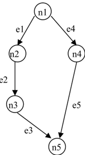
Another more applicable and general way to model a student’s action is by using the Bayesian Network (BN) (Yoo, Li, & Pettey, 2005). Bayesian Network is a directed acyclic graph (DAG) represented by BN=(V,E), where V is the nodes in this network, and E is the directed edges, see Figure 2.3. The edge between two nodes indicates the causal relation between them. When the directed edge e₁ goes from one concept node

1

n to another concept node n₂. Then this means n₁ should be met before n₂ happens.

(21)

8

Figure 2.3 An illustrative simple Bayesian Network.

Because the probability of reaching a current node depends only on its parent, the probabilities of the interested nodes can be calculated through the Joint Probability Distribution (JPD), and can be represented as

∏

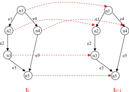
= = n i i i n P n Parent n n n n P 1 2 1, ,..., ) ( | ( )) (

In ITS systems, this means that the current student's learning state is influenced by his previous state and current system's suggestions. However, this graph is static and cannot change with the student’s learning states (i.e., add or remove some concepts into the student’s learning configuration). In order to tackle this problem, we must take the change over time into consideration, as suggested in Dynamic Bayesian Networks (DBN). The main idea of DBN is that the causal edges will update as time goes by. In addition to dealing with the relations among nodes, we must also consider the states in the next time ti+₁ and current time ti (see Figure 2.4).

n5 n4 n1 e3 e2 n3 n2 e1 e5 e4

(22)

Figure 2.4 Dynamic Bayesian Network changes with time.

There are some variations of the (Dynamic) Bayesian Network; for example, Dynamic Feedback and Multi-layered Inferencing Student Model in the following subsections.

2.7.1 Dynamic Feedback

This strategy talks about how to relate an incorrect student action to a correct action based on real-time comparisons between the current student and the expert actions. 2.7.2 Multi-layered Inferencing Student Model

This model comes from Woolf’s research (Woolf & Murray, 1994). Each layer contains a set of symbolic values, and takes inputs (the prerequisite knowledge) of lower layer and output (known or unknown binary value of this concept) to upper layer, where each layer represents the required concept of the domain.

n5 n4 n1 e3 e2 n3 n2 e1 e5 e4 n5 n4 n1 e3 e2 n3 n2 e1 e5 e4

t

i

t

i+1

(23)

10

2.8 Classification and Clustering

There are many clustering algorithms (Legaspi, 2002; Vos, 2002; Wickramasinghe & Alahakoon, 2004; Helmy & Shahab, 2006) designed to classify the students’ raw data. We can then use the classifier to judge whether or not the student knows some concept. Here, we just mention two most popular methods – Regression Model (i.e., for linear cases) and Support Vector Machine (SVM) (i.e., for non-linear cases).

2.8.1 Regression Model

The simplest system model in ITS is called the regression model (Beck, Stern, & Woolf, 1997). The authors use the regression model to identify whether a student overestimates or underestimates himself/herself through the self-explanation of his/her own ability and proficiency. The Regression equation used to approximate the student's action from his/her current action (A), expert's suggestion (B), and parameter adjustment (c), is

Student Performance = a*A + b*B + c where parameter a and b is the weight of A and B, respectively. 2.8.2 Support Vector Machine

The state-of-the-art method to classify the raw data into different clusters or groups is the Support Vector Machine (SVM) algorithm (Haydemar, Cecilio, & Andreu, 2002). SVM transforms the complicated multi-dimensional raw data vectors into hyperplane (feature space) to simplify and classify it, and then map it back to original dimensions. The classification curve is not like the linear regression model (the simplest case of

(24)

SVM). The shape may be irregular and this method is often used when encountering large amount of raw data.

2.9 Genetic Algorithms

The reason why we need Genetic Algorithms (GA) (Chen, Hong, & Chang, 2006) is due to its evolutionary advantage. The authors use GA to generate the personalized and optimal learning path much like the Curriculum Sequencing mentioned in Section 3.1. The evolution of GA here depends on their proposed Fitness Function. This function considers the concept relation degree and the difficulty parameter of the courseware at the same time, and then finds the summation of the weights of these two factors. The more relevant the concept relation degree is, the higher the value of the Fitness Function.

2.10 Summary

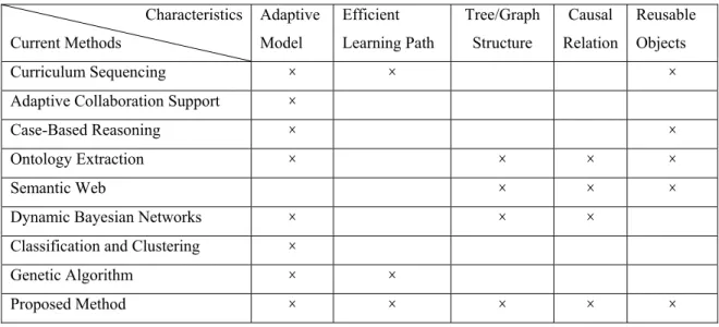
The main differences between the strategies above are summarized in Table 2.1. From this table, we can see that adaptive system model, personalized learning path, relational concept tree structure, and object-reusable property are the main trends for the development of next-generation intelligent tutoring systems.

(25)

12

-Table 2.1 Comparative study of different approaches. *The field indicated by “×” means the method has this feature.

Characteristics Current Methods Adaptive Model Efficient Learning Path Tree/Graph Structure Causal Relation Reusable Objects Curriculum Sequencing × × ×

Adaptive Collaboration Support ×

Case-Based Reasoning × ×

Ontology Extraction × × × ×

Semantic Web × × ×

Dynamic Bayesian Networks × × ×

Classification and Clustering ×

Genetic Algorithm × ×

(26)

In this study, based on the applied application (PLC), we proposed a new intelligent tutoring system architecture which incorporates the above structures and includes new features. For example, we built the concept tree structure (domain ontology), and identified the relations among the concepts to let the tutoring system know current required concepts and efficiently jump to the problems in the student’s classification level.

In addition, we proposed a strategy to keep making the database increasingly complete by storing experiment participants’ configurations and concepts into it. Moreover, we used Macromedia Flash MX, PHP 5, Java, and JavaScript to do the programming. The communication between the client and the server is through the Apache server, and the system uses Microsoft Access 97 database to store all the participants’ information.

Also, in our system implementation, we used the Object-Oriented Programming (OOP) design style to create the objects once and included them for all subsequent program development, thus saving memory space and reducing server execution time.

(27)

14

CHAPTER III METHODOLOGY

3.1 Introduction

In the previous chapter, we reviewed research related to possible solution areas for the research questions defined in Section 1.1 and introduced future perspectives which we will cover in this investigation. These areas include the adaptive model, tree structure, and reusable objects. Specifically, in this chapter we will apply the learning algorithm to solve the research problem and give an illustrative example to explain our proposed method. The complete system architecture and its interface design will be explained in the next chapter.

3.2 Assumptions

Before we talk about our proposed algorithm, it is important to mention the assumptions first. One of our assumptions is that we build some collaborative user records into the database. These records also known as patterns are used for finding the most similar or matching pattern to the current user’s rung configuration. For each problem in our domain, there are different numbers of built-in patterns for it.

In addition to the built-in user patterns, when talking about the intelligent tutoring system as follows, we made another two assumptions. First, the ITS knows all the required concepts for this Programmable Logic Controller domain already; second, the ITS knows which concepts need which subconcepts.

(28)

3.3 Learning Algorithm

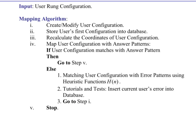
Figure 3.1 shows our learning algorithm for the intelligent tutoring system. The current user’s rung configuration is taken as the input, and then the system stores this configuration into the database. Before mapping this configuration with the existing patterns, the system will recalculate the coordinates of each component in this configuration and then compare this recalculated configuration with the answers. If the configuration is the same as one of the answers, the student will be congratulated and will move on to the next problem. If the configuration is wrong, the system will use heuristic functions to discern the most similar patterns and guide the student to solve his/her errors step-by-step, for example, by providing tutorials and tests of the error concepts and highlighting the error locations of the current configuration with pink color.

When he/she chooses one of the error concepts to go into the tutorial to learn it (and then test it), the system will store this concept combined with the current configuration into the database. The system database will become increasingly complete by recording students’ rung configurations and error concepts they made. The more complete the database becomes, the more accurate matching pattern the system can find.

(29)

16

Figure 3.1 Learning algorithm of Intelligent Tutoring System.

Input: User Rung Configuration.

Mapping Algorithm:

i. Create/Modify User Configuration.

ii. Store User’s first Configuration into database. iii. Recalculate the Coordinates of User Configuration. iv. Map User Configuration with Answer Patterns:

If User Configuration matches with Answer Pattern Then

Go to Step v. Else

1. Matching User Configuration with Error Patterns using Heuristic FunctionsH(n).

2. Tutorials and Tests: Insert current user’s error into Database.

3. Go to Step i. v. Stop.

(30)

3.3.1 Heuristic Functions

In our current work, we develop heuristic functions to map the current student’s error sequences with existing error patterns in the Knowledge Base. Based on the Programmable Logic Controller application, our developed heuristic functions are listed in Figure 3.2. : _ Re ) ( 1 n dundant Component h = -1 (1) Difference Length Rung Difference Length Rung n h₂( )= _ _ :− _ _ (2) = ) ( 3 n h Matching_Component_and_Examined_Bit: +1 (3) : _ ) ( 4 n Misplaced Component h = -|Position_Diff_of_Component| (4) = ) ( 5 n h Misplaced_Examined_Bit: -|Position_Diff_of_Examined_Bit| (5)

∑

= = 5 1 ) ( ) ( i i n h n H (6)

Figure 3.2 Heuristic functions.

In this figure, Equation (1) means that if there is any redundant component in the current configuration (i.e., wrong examined bit or selected logic), one will be subtracted from the total score. Equation (2) compares the current configuration with the answer patterns, and if there is any length difference between each rung, the total score will also be subtracted by the total difference of the rung length. Equation (3) tries to discern the same examined bit and logic of components when comparing the answers. The total score will increase by one if the function finds one matching component in the current configuration. Equation (4) and (5) discern the matching components and examined bits that are misplaced, and the total score will decrease by the sum of these misplaced

(31)

18

components (i.e., each misplaced component or misplaced examined bit will lead to a decrease of one). Our accumulative heuristic function H(n) is listed as equation (6). 3.3.2 An Illustrative Example

The following is an example of how to apply our heuristic functions to the rung configurations of Programmable Logic Controller (PLC) application, and mapping the current user’s wrong rung configuration to one of the existing rung patterns in the ITS database.

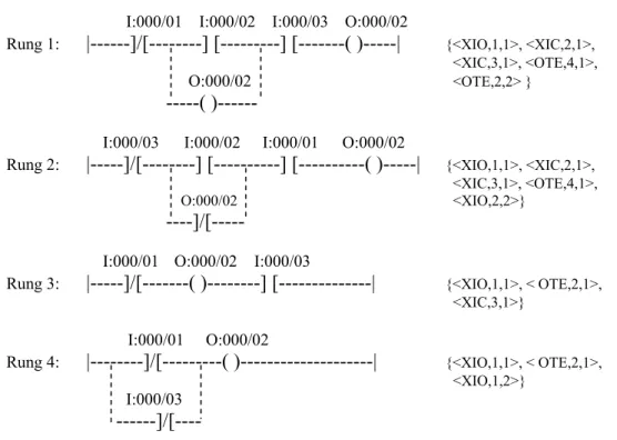
Figure 3.3 shows the built-in PLC rung configurations and mapping sequences (tuples) in the database. The coordinates in the mapping sequences are based on the scan sequence of the user’s rung configuration (i.e., from left to right first and then top to down).

Table 3.1 shows the calculation of the utility (total score) of our proposed heuristic functions. The utility is derived from the sum of five different heuristic functions. From the result shown in Table 3.1, we can see that the current student’s error rung configuration maps to Rung 3 (i.e., the utility of Rung 3 is the highest).

(32)

Rung Configuration in PLC Mapping Sequence in the Database I:000/01 I:000/02 I:000/03 O:000/02

Rung 1: |---]/[---] [---] [---( )---| {<XIO,1,1>, <XIC,2,1>, <XIC,3,1>, <OTE,4,1>, O:000/02 <OTE,2,2> }

---( )---

I:000/03 I:000/02 I:000/01 O:000/02

Rung 2: |---]/[---] [---] [---( )---| {<XIO,1,1>, <XIC,2,1>, <XIC,3,1>, <OTE,4,1>,

O:000/02 <XIO,2,2>}

----]/[---

I:000/01 O:000/02 I:000/03

Rung 3: |---]/[---( )---] [---| {<XIO,1,1>, < OTE,2,1>, <XIC,3,1>}

I:000/01 O:000/02

Rung 4: |---]/[---( )---| {<XIO,1,1>, < OTE,2,1>, <XIO,1,2>}

I:000/03 ---]/[----

Current Student’s error rung configuration: I:000/01 I:000/03 O:000/02

Rung : |--- ( )---][---]/[---| {<OUT,1,1>, <XIC,2,1>, <XIO,3,1>}

(33)

20 Table 3.1 Calculation of heuristic functions H(n).

Rung # Redundant

Component Length Difference Matching Component and Examined Bit Misplaced Logic Component Misplaced Examined Bit H(n)

1 -2 -|3-4|= -1 +1 -|1-4| - |2-2| - |3-1| = -5 -|1-1| - |2-3| - |3-4| = -2 -9 2 -2 -|3-4|= -1 +1 -|1-4| - |2-2| - |3-1| = -5 -|1-3| - |2-1| - |3-4| = -4 -11 3 0 -|3-3|= 0 +1 -|1-2| - |2-1| - |3-1| = -4 -|1-1| - |2-3| - |3-2| = -2 -5* 4 -1 -|3-2|= -1 0 -|1-2| - |2-0| - |3-1| = -5 -|1-1| - |2-1| - |3-2| = -2 -9

(34)

3.4 Proposed System 3.4.1 System Architecture

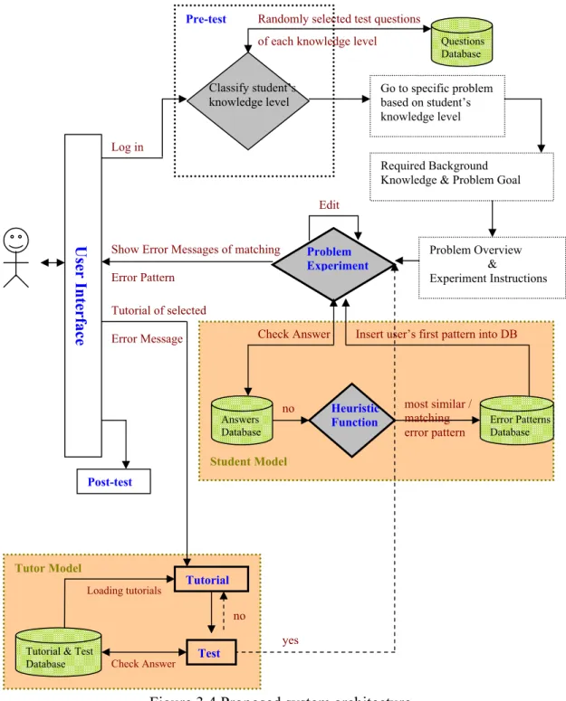
After extensively examining the pros and cons of intelligent tutoring systems in Chapter II, we want to propose our system architecture as an effective means of achieving the research objectives listed in Chapter I. Our overall system architecture is shown in Figure 3.4, and the detail relations between the components of the architecture are described in the following sections.

3.4.2 User Interface

When it comes to student learning, we cannot put all the concentration on the backend system development. The user interface is also important; it should be designed in a manner that attracts students’ interest, and should encourage students’ long-term retention of the concepts through the vivid animations of the user interface. Thus, the layout of the user interface is given much consideration here. A learning style questionnaire was conducted prior to the design of the ITS prototype. Figure 3.5 shows the learning preference distribution of 12 participants who voluntarily took this questionnaire. The X-axis of the distribution indicates the preference for visualized learning or verbal learning. A higher X-axis index means the student prefers more verbal and less visualized tutoring. A lower X-axis index means the student prefers less verbal and more visualized tutoring. From this bar chart distribution, we can see that the students desire more visualized pictures and diagrams when they are learning some domain knowledge.

(35)

22

Figure 3.4 Proposed system architecture.

Pre-test Student Model Tutor Model Post-test User Interface Go to specific problem based on student’s knowledge level Classify student’s knowledge level Questions Database Randomly selected test questions

Log in

Required Background Knowledge & Problem Goal

Problem Overview & Experiment Instructions Problem Experiment Answers Database Check Answer most similar / matching

error pattern Error Patterns Database no Heuristic

Function

Edit

Tutorial of selected

Error Message Insert user’s first pattern into DB Show Error Messages of matching

Error Pattern

Tutorial

Test

no

yes

of each knowledge level

Tutorial & Test

Database Check Answer Loading tutorials

(36)

Learning Preference Distribution 0 1 2 3 4 5 6 1 2 3 4 5 6 7 8 9 10 11 Visual vs. Verbal num be r of s tu de nt s

Figure 3.5 Student learning preference distribution.

Our current modified ITS is designed according to the system evaluation feedback and learning style of the voluntary participants and is much more friendly and understandable than our prototype design. In addition to pictorial illustration of problems, we also include the animations of switch control of Virtual Programmable Logic Controller (VPLC) to help students easily discover solutions for the problems.

3.4.3 Pre-test

Instead of making the assumption that every student does not know the concepts in this PLC domain, we prefer to offer a dynamic pre-test to learn and classify the students into different levels – beginner, intermediate, or professional – in the beginning. The questions of the pre-test will be generated one by one, and the generation of each question is based on the answer of the previous question the students answer. The difficulty of the questions asked are in accordance with the level in which they are categorized, and are randomly drawn to test the student’s knowledge. The student will be

(37)

24

tested beginning with the simplest concept about PLC, and then the system will gradually adjust the concept difficulty to determine the extent of the student’s knowledge. In our testing procedure, the student will be asked questions of the next difficulty level if and only if he/she answers two questions correctly in a row.

3.4.4 Problem Selection

In our evaluation system, we develop ten problems, named from Problem1 to Problem10, to help students become familiar with the possible situations in which they might apply the PLC concepts. These ten problems are carefully selected from commonly used PLC experiment laboratories, and classified into three different levels based on the difficulties of solving them. In our system classification, Problem1 and Problem2 belong to knowledge level one – beginner level. Problem3 to Problem5 belong to the second knowledge level – intermediate. The third knowledge level – professional – includes Problem6 to Problem10. The required concepts of each problem are listed in Table 3.2. Each concept in this table will be explained in Section 4.2 where we will talk about the introduction to ladder diagram programming.

(38)

25 Table 3.2 Predefined student knowledge level and concepts classification.

Classified Problems Required Concepts for each Problem

Problem1 XIC, XIO, OTE, NO, NCSR, NOSR, Examined Bit, Parallel/Serial Structure

Knowledge Level 1

Problem2 XIC, XIO, OTE, NO, NCSR, NOSR, Examined Bit, Parallel/Serial Structure

Problem3 XIC, XIO, OTE, NO, NCSR, NOSR, Examined Bit, Parallel/Serial Structure,

Lock/Unlock switch

Seal State Knowledge Level 2

Seal State, Closed Circuit

Seal State, Closed Circuit, EN bit, DN bit, Preset value, Accum value, Timer Base, TON, TOF, CTU

Knowledge Level 3

(39)

26

The relations among the concepts used in these ten problems are shown in Figure 3.6 as a Directed Acyclic Graph (DAG). The required concepts for testing these 10 Flash problems are displayed in this network where the difficulty of the concepts grows with the number of the levels. Furthermore, the directed edge from one node (A) to another node (B) means that before doing B, A must be learned first. The system will bring the student to different problems based on his/her pre-test result, and then will go through the subsequent problems until the student finishes the last problem (Problem10).

The figure also indicates that there are three knowledge levels – beginner, intermediate, and professional – in the ITS design. We can see that Problem1 and Problem2 belong to the beginner level (Knowledge Level 1), Problem3 to Problem5 belong to intermediate level (Knowledge Level 2), and Problem6 to Problem10 are in the professional level (Knowledge Level 3). The classifications of these 10 problems are totally based on the difficulties of the domain concepts. When the student moves from the current level to the next level, the problems in the next level will contain more concepts and are harder than those in the current level.

(40)

Level 1 Level 2 Level 3 Level 4 Level 5 Level 6 Level 7 Level 8 Level 9

Figure 3.6 Directed acyclic graph, where white circles means concepts and yellow rectangles represent 10 Flash PLC problems, respectively.

XIC XIO OTE

Basic

Examined Bit Parallel structure Serial structure

#1 #2 #3 #4 #9 #6 #7 #8 #10 DN EN Preset Accum

CTU Timer Base

TON TOF Seal state Lock/Unlock #5 Closed circuit beginner intermediate professional (Hardware Knowledge) (Logics Knowledge)

(41)

28

3.4.5 User Sequence Generation

After the student reads the statement of each problem, he/she will try to manipulate the toolbox to create some rung configuration in the working area. Then, the system will send this configuration from the client side to the server side and store this configuration into the database. The transfer of the configuration into the records in the database is based on the location, or coordinate, of each component. The coordinate mapping and detail system interface will be explained further in Chapter IV. In the sections below, the comparison and mapping of different configurations are mainly based on the coordinate of each component.

3.4.6 Answer Comparison

Sections 3.4.6 to 3.4.9 are explained by the system flowchart shown in Figure 3.7. After the student completes the current problem’s configuration, the system will compare this configuration with each of the answers in the database. This comparison includes the location, logic, and examined bit of each component in this configuration. If components in the current configuration are totally matched with the components in one of the possible answer patterns, the system will congratulate the student and bring him/her to the next problem. If the current user configuration is incorrect, the system will compare this configuration with existing error patterns in the database using heuristic functions.

(42)

Figure 3.7 System flowchart.

yes 1. Matching correct sequence. 2. Go to similar/harder question.

matching with correct sequences in DB

no

Using Heuristic function H(n) to match with error sequences in DB

yes

Based on the possible concept errors of the matching error sequence, go to selected error concept.

no

Jump to the tutorial of this concept/misconception.

Test this concept/misconception yes

no

1. Insert current error sequence into DB. 2. Record this error.

next Post-test

exit

next next

(43)

30

3.4.7 Mapping with Heuristic Functions

In order to discern the most similar or matching student pattern related to the current user’s configuration, we embed heuristic functions inside the Student Model to approximate the error pattern that has the closest similarity. Once the most similar error pattern is identified, the incorrect or misunderstood concepts of that error pattern will be shown to the user. The user will then have a better understanding of what concepts he/she is not clear about.

Once the student runs the program to execute his/her rung configuration, the system will insert his/her configuration into the Error Patterns table in Microsoft Access 97 database first, and then keep recording the concepts he/she chooses to learn during the problem experiment stage. The Error Patterns table will have growing error patterns and will have higher accuracy pinpointing the errors for the coming users’ rung configurations.

3.4.8 Tutorials and Tests

Based on the displayed error concepts mentioned in section 3.4.7, the student will choose any of his/her misunderstood concepts. The Tutor Model will then bring up the tutorials of the selected error concept, teach the student the concept carefully and comprehensively, and then generate some test questions to evaluate the student’s understanding of this concept. Once the student has learned the concept by passing the concept test questions, the system will bring the student back to the original problem to let the student do the experiment again.

(44)

3.4.9 Pre-exam and Post-exam

In order to evaluate the performance of our developed ITS, we mounted our tutoring system on the server, and allow everyone who can access the internet to test it. The participants are voluntary for this system evaluation and are anonymous.

Before the participants use the ITS to increase their understanding of PLC concepts, we let them take the paper exam (pre-exam) first. The problems in this exam will test the participants’ knowledge about PLC concepts on which they will be tutored in this ITS.

After the participants finish all the problems in the ITS including tutoring and debugging of these problems provided by the intelligent system, we give the participants another paper exam (post-exam). Each problem has the same required concepts as the problems in the original pre-exam, but has different problem designs that asking the same question in a different way in an effort to test their knowledge level again. We then grade this post-exam and compare the test grade of the post-exam with the pre-exam to determine how much the student learned from this intelligent tutoring system. In our current results, we found three participants to do the system evaluation.

(45)

32

CHAPTER IV

SYSTEM IMPLEMENTATION

4.1 System Programming and Environment Setting

In our system implementation, we use PHP 5 Scripting language, Macromedia Flash 2004 ActionScript language, Java, JavaScript, Apache 2 Server, and Microsoft Access 97 database (see Figure 4.1) to build the intelligent system. The complete hierarchical function list is shown in the Appendix. Once the student gets into the experiment window, does some drag-and-drop actions to finish his/her configuration, and then runs the program, the system will send the configuration stream from the client side to the server side. Then, the PHP scripts behind the Apache server will execute the required calculations and comparisons to store/retrieve data from the Access 97 database. The results will then be sent back to the client side.

Figure 4.1 Programming tools and program execution flow.

Server Side Flash ActionScript

JavaScript Client Side

Apache 2

Server Microsoft Access 97

internet PHP5

Scripts

Store & Retrieve data

(46)

During summer 2006, we developed a VPLC system that contains 10 Flash problems. For each of these 10 problems, there is first a problem statement and operation instructions, and then the students will do the drag-and-drop operations to complete the rung configuration. In this system, when the student makes some errors, the ITS just provides related feedback that tells what and where errors might exist and then leaves the errors for the student to solve. In our current work, we try to implement the heuristic functions to map the current user’s error pattern with existing error patterns in the Student Model. Then, based on the most similar/matching error pattern, we guide the current student through his errors based on the errors in the matching pattern.

4.2 Introduction to Programming Logic Diagrams 4.2.1 Ladder Diagram Introduction

Given the problem statement, the goal of ladder diagrams is to assign the rung configuration I/O ports and logic components to meet the requirements of the problem statement. If there is some problem with the configuration, the user will need to re-edit and verify the program.

4.2.2 Included Ladder Diagram Concepts

In our thesis research, we extract the most important and commonly used logic components in the PLC problems and put them into our intelligent tutoring system. These logics include Examine if Closed (XIC), Examine if Open (XIO), Output Energize (OTE), Timer On-Delay (TON), Timer Off-Delay (TOF), and Count Up (CTU); these are all explained in Tables 4.1 and 4.2.

(47)

34 Table 4.1 Detail explanation of PLC software components.

Enable Bit (EN) EN bit is set when rung conditions are true, and remains set until rung

conditions go false.

Timing Bit (TT) TT bit is set when rung conditions are true, and is reset when run conditions

go false or when the DN bit is set.

Done Bit (DN) DN bit is set when accumulated value is equal to or greater than the preset

value. The DN bit is reset when rung conditions go false.

Count Up Enable Bit (CU) CU bit is set when rung conditions are true, and remain set until rung

conditions go false. Examined Bit

Count Reset Bit (RES) Use a RES instruction to reset a timer or counter.

---] [--- Examine if Closed (XIC).

Use the XIC instruction in your ladder program to determine if a bit is On.

---] / [--- Examine if Open (XIO).

Use an XIO instruction in your ladder program to determine if a bit is Off.

---( )--- Output Energize (OTE).

Use an OTE instruction in your ladder program to turn On a bit when rung conditions are evaluated as true.

TON --- PR 3600 ---

AC 0

Timer On-Delay (TON).

Use the TON instruction to delay the turning on or off of an output.

TOF

--- PR 7000 --- AC 0

Timer Off-Delay (TOF).

Use the TOF instruction to delay turning on or off an output. Logic

CTU --- PR 5 ---

AC 0

Count Up (CTU).

(48)

35 Table 4.2 Detail explanation of PLC hardware components.

Normally Open (NO).

The NO switch enables the input pin when it is closed, and disables it when it is open.

Normally Closed (NC).

The NC switch enables the input pin when it is closed, and disables it when it is open.

Normally Closed Spring Return (NCSR).

Similar to NO switch, NCSR switch enables the input pin when it is released, and disables it when it is pressed.

Switch

Normally Open Spring Return (NOSR).

Opposite to the NCSR switch, NOSR switch enables the input pin when it is pressed, and disables it when it is released.

(49)

36

4.2.3 An Example of the Rung Configuration

An example of one simple rung configuration is shown in Figure 4.2. The way the system scans the rung configuration is from left to right and then top to down, and the enable/disable status of each location is identified through the selected examined bit and logic component. In order to make the location enabled, both the selected examined bit and selected logic component should be correct. Should any one of them be incorrect, it will disable the location. The example configuration also includes a parallel structure – SW6 component – which provides another path to enable the logic component behind it, in this case, Fan.

Figure 4.2 An example of the rung configuration. In this rung configuration, L1 and L2 represent lights, and SW6 represents switch #6.

L1

L2

Fan

I:000/01

I:000/02

O:000/02

---] [---] [---( )---

SW6

I:000/03

(50)

4.3 User Configuration Mapping

After introducing a simple rung example in Section 4.2.3, now we look deeper into the implementation strategy of our system. Sections 4.3.1 to 4.3.3 detail the explanation of our implementation strategy, including coordinate mapping, coordinate recalculation, and path enable/disable determination.

4.3.1 Coordinate Mapping

Our backend design of the working area is composed of five hidden complicated rung structures, one of which is shown in Figure 4.3. Each hidden rung structure has an identical shape but different location indices. Each hidden rung structure contains 20 locations, and each location is assigned a unique (X, Y) value. These unique (X,Y) values are used to remember the ordering of each location and also for the coordinate recalculation.

Figure 4.3 System working area setting of one of the hidden rungs.

--- --- ---

-- - -

-- --- --- -- ---- --- -- ---

-- -- --

-- --- --- -- ---- --- ---

1,1 2,1 3,1 4,1 5,1 6,1 1,2 2,2 3,2 4,2 5,2 6,2 1,3 2,3 3,3 4,3 5,3 6,3

(51)

38

4.3.2 Coordinate Recalculation

Suppose the user has finished his/her rung setting. The system will use the (X,Y) values to rearrange the placement of the existent locations; it will remove the blank/hidden locations, and also reassign the (X,Y) values to these locations (see Figure 4.4 and 4.5).

Figure 4.4 Before coordinate recalculation of one of the hidden rungs. Suppose the gray areas represent the logics and examined bits configured by the user.

Figure 4.5 After coordinate recalculation of one of the hidden rungs.

--- --- ---

--

--1,1 2,1 3,1 2,2

--- --- ---

-- - -

-- --- --- -- ---- --- -- ---

-- -- --

-- --- --- -- ---- --- ---

1,1 2,1 3,1 4,1 5,1 6,1 1,2 2,2 3,2 4,2 5,2 6,2 1,3 2,3 3,3 4,3 5,3 6,3

(52)

4.3.3 Path Enable/Disable Determination

After the coordinate recalculation process, the system will then display the enable/disable status of each component. For the components that are not output logics, such as XIC and XIO, the enable/disable status of them is determined by their examined bits and logic components, for instance, the (1,1), (2,1), and (2,2) locations in Figure 4.6. For other components, in this case, the (3,1) location in Figure 4.6, the enable/disable status of them is based on the components before it on the path. For example, if we want the (3,1) location to be enabled, the locations in the red path – (1,1) and (2,1) – or the green path – (1,1) and (2,2) – should both be enabled.

Figure 4.6 Path enable/disable determination of one of the hidden rungs.

--- --- ---

-- --

1,1 2,1 3,1

(53)

40

4.4 System Layout Snapshot

Our system snapshot of the main page is shown in Figure 4.7. We divide this figure into different parts with each enclosed in a red rectangle, and explain the function of each of them as follows. The placement of each area is from the feedback of the evaluation participants. Area A shows our virtual design of the Programmable Logic Controller. The left-hand side of it includes the input pins and the control switches; the right-hand side of it includes the output pins and output devices (i.e., fans in this system snapshot). Area B gives a quick review of the problem statement and also instructions on how to manipulate the toolbox shown in Area E. Area D lists all buttons that will be used to configure the user’s setting. The user will use the toolbox to complete his/her configuration in Area F, and then click the Run button in Area D to test his/her configuration. When executing the user’s rung configuration, the ITS system will do some calculations and comparisons to discern the answer or matching error pattern. To help the user identify mistakes in the user configuration, the system will present possible physical errors by highlighting rectangles shown in Area F, and giving suggestions for related concepts that the user might not know and might help the user to solve the errors in Area C.

(54)

41 Figure 4.7 System snapshot of the experiment window.

A

B

C

E F

(55)

42

CHAPTER V

EVALUATION AND RESULTS 5.1 Introduction

For the system evaluation, we put the web-based system on the public internet, and allow users all over the world to access the system and learn the domain knowledge from it. We then evaluated our system’s performance through an analysis of participating users’ learning progress, including such factors as learning time for each problem and posterior questionnaire after participants finish their work. We also developed our simulation model to simulate the relationship of students’ proficiency and problem-solving time described in Section 5.2.4. The justification of robustness of the learning algorithm and system adaptivity is also demonstrated through the experiments described in Sections 5.2.1 and 5.2.2.

Our expected result is that this web-based system will help students quickly and efficiently learn the PLC concepts and give them an enormous feeling of satisfaction.

5.2 Simulation Experiments and Results

For our system evaluations, we design experiments and evaluation that include the learning algorithm robustness testing, and system adaptivity testing, participant evaluation, and system model simulation; each of which will be explained in the following four sub-sections.

5.2.1 Heuristic Function Accuracy

(56)

of heuristic functions. Our hypothesis is that there is a function effect on matching the accuracy of error patterns, and by applying different combinations of our proposed heuristic functions, we can get diverse accuracy measurements.

Our method is to classify possible user configurations based on the error concepts first and then randomly generate trial user configurations for each classified combination of error concept(s). We use these randomly generated trial user configurations to run different combinations of heuristic functions to determine the mapping result. Table 5.1 enumerates all possible combinations of error concepts required to solve Problem1 and also gives corresponding rung configurations to these concepts; Table 5.2 shows matching patterns and mapping results of randomly generated trial user configurations for the combinations of error concepts for Problem1.

Table 5.3 shows the results of our experiment, where HF1 means the simplest heuristic function, and HF5 represents the most complete one. Each of the calculated results in the table derives from the ratio of matching patterns to all trial user configurations. Figure 5.1 visualizes the data in Table 5.3. From this figure, we can see that HF5 has the best accuracy for each problem, almost 90 percent accuracy on average. That is, with the increasing number of proposed heuristic functions, the mapping result will become more and more accurate.

(57)

44 Table 5.1 Error patterns of Problem1.

index

Combinations of

Error Concepts Error Patterns for this Concept Pattern Name

1 XIC I:000/01 O:000/02

|---] / [---( )---| | I:000/03 |

---] / [---

User0101

2 XIO I:000/01 O:000/02

|---] [---( )---| | I:000/03 |

---] [---

User0102

3 OTE I:000/01 O:000/02

|---] [---] [---| | I:000/03 |

---] / [---

User0103

4 Examined Bit I:000/03 O:000/02

|---] [---( )---| | I:000/03 | ---] / [--- User0104 5 Parallel/Serial Structure

I:000/01 I:000/03 O:000/02

|---] [---] / [---( )---|

User0105

6 XIC + XIO I:000/01 O:000/02

|---( )---( )---| | I:000/03 |

---( )---

(58)

45 Table 5.1 Continued. index Combinations of Error Concepts

Error Patterns for this Concept Pattern Name

7 XIC + OTE I:000/01 O:000/02

|---] / [---] / [---| | I:000/03 |

---] / [---

User0107

8 XIC +

Examined Bit I:000/03 O:000/02 |---] / [---( )---|

| I:000/03 | ---] / [--- User0108 9 XIC + Parallel/Serial Structure

I:000/01 I:000/03 O:000/02

|---] / [---] / [---( )---|

User0109

10 XIO + OTE I:000/01 O:000/02

|---] [---] [---| | I:000/03 |

---] [---

User0110

11 XIO +

Examined Bit I:000/03 O:000/02 |---] [---( )---|

| I:000/03 | ---] [--- User0111 12 XIO + Parallel/Serial Structure

I:000/01 I:000/03 O:000/02

|---] [---] [---( )---| User0112 13 OTE + Examined Bit I:000/03 O:000/02 |---] [---] [---| | I:000/03 | ---] / [--- User0113

(59)

14 OTE +

Parallel/Serial Structure

I:000/01 I:000/03 O:000/02

|---] [---] / [---] [---| User0114 15 XIC + XIO + Examined Bit I:000/03 O:000/02 |---( )--- ( )---| | I:000/03 | ---( )--- User0115 16 XIC + XIO + Parallel/Serial Structure

I:000/01 I:000/03 O:000/02

|---( )--- ( )--- ( )---| User0116 17 XIC + OTE + Examined Bit I:000/03 O:000/02 |---] / [---] / [---| | I:000/03 | ---] / [--- User0117 18 XIC + OTE + Parallel/Serial Structure

I:000/01 I:000/03 O:000/02

|---] / [---] / [---] / [---| User0118

19 XIO + OTE +

Examined Bit I:000/03 O:000/02 |---] [---] [---|

| I:000/03 |

---] [---

(60)

20 XIO + OTE +

Parallel/Serial Structure

I:000/01 I:000/03 O:000/02

|---] [---] [---] [---| User0120 21 XIC + XIO + Examined Bit + Parallel/Serial Structure

I:000/03 I:000/03 O:000/02

|---( )--- ( )--- ( )---| User0121 22 XIO + OTE + Examined Bit + Parallel/Serial Structure

I:000/03 I:000/03 O:000/02

|---] [---] [---] [---| User0122

23 XIC + OTE +

Examined Bit + Parallel/Serial

Structure

I:000/03 I:000/03 O:000/02

|---] / [---] / [---] / [---|

(61)

48 Table 5.2 Matching patterns and accuracy measurements of Problem1.

Matching Pattern / Accuracy

Index Combinations of Error Concepts

HF1 HF2 HF3 HF4 HF5

User0101 User0101 User0101 User0106 User0106

1 XIC

+ + + + +

2 XIO

+ + + + +

3 OTE

+ + + + +

4 Examined Bit

+ + + - +

5 Parallel/Serial Structure

- - - - -

6 XIC + XIO

+ + + + +

7 XIC + OTE

+ + + + +

8 XIC +

Examined Bit _- ₊ ₊ ₊ ₊

9 XIC + Parallel/Serial Structure

- - - + +

10 XIO + OTE

(62)

49 Table 5.2 Continued.

HF1 HF2 HF3 HF4 HF5

11 XIO +

Examined Bit _- _- ₊ ₊ ₊

12 XIO + Parallel/Serial Structure

+ + + + +

13 OTE +

Examined Bit _- _- _- _- ₊

14 OTE + Parallel/Serial Structure

+ + - - +

15 XIC + XIO + Examined Bit

- - - - -

16 XIC + XIO + Parallel/Serial

Structure _- _- ₊ ₊ ₊

17 XIC + OTE + Examined Bit

- - - + +

18 XIC + OTE + Parallel/Serial

Structure _- ₊ ₊ ₊ ₊

19 XIO + OTE + Examined Bit

- - - - +

20 XIO + OTE + Parallel/Serial

Structure _- _- ₊ ₊ ₊

21 XIC + XIO + Examined Bit +

(63)

50 Table 5.2 Continued.

HF1 HF2 HF3 HF4 HF5

22 XIO + OTE + Examined Bit +

Parallel/Serial Structure _- _- ₊ ₊ ₊

23 XIC + OTE + Examined Bit +

Parallel/Serial Structure _- _- _- _- ₊

Matching Patterns/Total Tests 8/23 10/23 13/23 15/23 21/23

(64)

51 Table 5.3 Use different number of heuristic functions to find the average mapping accuracy. Each of the calculated results in

the table derives from the ratio of matching patterns to all trial user configurations. Average Accuracy Number of Error Patterns _{HF1 HF2 HF3 HF4 HF5} Problem1 23 .35 .44 .57 .65 .91 Problem2 23 .32 .47 .63 .60 .88 Problem3 23 .38 .52 .66 .64 .92 Problem4 36 .27 .37 .53 .73 .82 Problem5 36 .31 .39 .49 .76 .90 Problem6 14 .36 .43 .56 .71 .83 Problem7 14 .24 .46 .48 .69 .86 Problem8 28 .34 .44 .53 .64 .85 Problem9 27 .29 .53 .56 .75 .88 Problem10 14 .18 .36 .51 .77 .84

(65)

52

Mapping Accuracy of Heuristic Functions

0 0.1 0.2 0.3 0.4 0.5 0.6 0.7 0.8 0.9 1 0 1 2 3 4 5 6

Different Heuristic Functions

A ver ag e A ccu ra cy o f E ach H eu ri st ic F un ct io n Problem1 Problem2 Problem3 Problem4 Problem5 Problem6 Problem7 Problem8 Problem9 Problem10

Figure 5.1 Mapping accuracy based on different number of heuristic functions. Indices of X-axis represent how many heuristic functions are applied for all 10 problem’s accuracy measure (i.e., HF1 to HF5, from left to right).

(66)

5.2.2 System Adaptivity

The objective of our last experiment analysis is to test system adaptivity. In order to evaluate this properly, we create three databases that contain different numbers of error patterns – DB1, DB2 and DB3 – and use the most complete heuristic function, HF5, to test the accuracy difference among these databases. In our experiment setting, DB3 contains the most error patterns, DB2 removes one-third of the error patterns in DB3, and DB1 removes half of the error patterns in DB2. The procedures to develop these three databases are listed as follows

1. Enumerate all possible combinations of error concepts for each problem. 2. Carefully design patterns for these combinations of error concepts. 3. Insert these patterns into the databases as built-in error patterns.

4. Carefully design trial user patterns for these combinations of error concepts.

5. Use the web-based tutoring system to test the heuristic function mapping accuracy of these trial user patterns.

From Table 5.4, we can see that each problem has different numbers of error patterns in DB1, DB2 and DB3, and the system will find increasingly similar error patterns when the databases contain more error patterns. Figure 5.2 demonstrates a graphic display of the data in Table 5.4. From this figure, we can see that for each problem, the mapping accuracy becomes more precise with the increasing number of error patterns. The indices on the X-axis, from left to right, indicate DB1, DB2 and DB3, respectively.

(67)

54 Table 5.4 Use HF5 to measure the average accuracy based on different databases. Each of the calculated results derives from

the average of 10 user configurations.

Number of Error Patterns / Average Accuracy

DB1 DB2 DB3 8 16 23 Problem1 .52 .74 .91 8 16 23 Problem2 .56 .68 .88 8 16 23 Problem3 .48 .65 .92 12 24 36 Problem4 .59 .67 .82 12 24 36 Problem5 .38 .76 .90 4 8 14 Problem6 .46 .79 .83 4 8 14 Problem7 .49 .72 .86 9 18 28 Problem8 .53 .69 .85 9 18 27 Problem9 .41 .81 .88 4 8 14 Problem10 .47 .71 .84

(68)

55

Accuracy Distribution of different databases

0 0.2 0.4 0.6 0.8 1 0 1 2 3 4 Different Databases A ver ag e A ccu ra cy Problem1 Problem2 Problem3 Problem4 Problem5 Problem6 Problem7 Problem8 Problem9 Problem10

Figure 5.2 System adaptivity based on different databases. Database 3 (DB3) has the most complete error patterns, Database 2 (DB2) removes one-third of the error patterns in DB3, and Database 1 (DB1) removes half of the error patterns in DB2.

(69)

56

5.2.3 Participant Evaluation

In the participant evaluation, we give the participants a pre-exam of 10 problems before they do the system experiment, and we then grade their answers. After they evaluate the system and complete all 10 problems, we let them take the paper exam again (post-exam), the problems of which cover the same required concepts as the problems in the original exam (pre-exam). The objective of the post-exam is to test the users’ understanding of the PLC concepts, and thus give us a performance measurement of our developed tutoring system.

Table 5.5 shows the learning performance of the evaluating participants. From the table, we can see that before using the tutoring system, the participants have knowledge proficiency between 0.5 and 0.7 (i.e., test scores are 52, 58, and 76). After the students use the tutoring system, it will help the students solve the 10 problems and learn all the required concepts. Figure 5.3 shows a graphic display of Table 5.5. We can see that the system improved the users’ understanding of PLC domain knowledge.