Solving support vector machine classification problems and their applications to supplier selection

(1)

SOLVING SUPPORT VECTOR MACHINE CLASSIFICATION PROBLEMS AND THEIR APPLICATIONS TO SUPPLIER SELECTION

by GITAE KIM

B.S., Hanyang University, 1998 M.S., Seoul National University, 2000

AN ABSTRACT OF A DISSERTATION

submitted in partial fulfillment of the requirements for the degree DOCTOR OF PHILOSOPHY

Department Of Industrial & Manufacturing Systems Engineering College of Engineering

KANSAS STATE UNIVERSITY Manhattan, Kansas

(2)

Abstract

Recently, interdisciplinary (management, engineering, science, and economics) collaboration research has been growing to achieve the synergy and to reinforce the weakness of each discipline. Along this trend, this research combines three topics: mathematical programming, data mining, and supply chain management. A new pegging algorithm is developed for solving the continuous nonlinear knapsack problem. An efficient solving approach is proposed for solving the -support vector machine for classification problem in the field of data mining. The new pegging algorithm is used to solve the subproblem of the support vector machine problem. For the supply chain management, this research proposes an efficient integrated solving approach for the supplier selection problem. The support vector machine is applied to solve the problem of selecting potential supplies in the procedure of the integrated solving approach.

In the first part of this research, a new pegging algorithm solves the continuous nonlinear knapsack problem with box constraints. The problem is to minimize a convex and differentiable nonlinear function with one equality constraint and box constraints. Pegging algorithm needs to calculate primal variables to check bounds on variables at each iteration, which frequently is a time-consuming task. The newly proposed dual bound algorithm checks the bounds of Lagrange multipliers without calculating primal variables explicitly at each iteration. In addition, the calculation of the dual solution at each iteration can be reduced by a proposed new method for updating the solution.

In the second part, this research proposes several streamlined solution procedures of -support vector machine for the classification. The main solving procedure is the matrix splitting method. The proposed method in this research is a specified matrix splitting method combined with the gradient projection method, line search technique, and the incomplete Cholesky decomposition method. The method proposed can use a variety of methods for line search and parameter updating. Moreover, large scale problems are solved with the incomplete Cholesky decomposition and some efficient implementation techniques.

To apply the research findings in real-world problems, this research developed an efficient integrated approach for supplier selection problems using the support vector machine and the mixed integer programming. Supplier selection is an essential step in the procurement

(3)

processes. For companies considering maximizing their profits and reducing costs, supplier selection requires seeking satisfactory suppliers and allocating proper orders to the selected suppliers. In the early stage of supplier selection, a company can use the support vector machine classification to choose potential qualified suppliers using specific criteria. However, the company may not need to purchase from all qualified suppliers. Once the company determines the amount of raw materials and components to purchase, the company then selects final suppliers from which to order optimal order quantities at the final stage of the process. Mixed integer programming model is then used to determine final suppliers and allocates optimal orders at this stage.

(4)

SOLVING SUPPORT VECTOR MACHINE CLASSIFICATION PROBLEMS AND THEIR APPLICATIONS TO SUPPLIER SELECTION

by

GITAE KIM

B.A., Hanyang University, 1998 M.S., Seoul National University, 2000

A DISSERTATION

submitted in partial fulfillment of the requirements for the degree DOCTOR OF PHILOSOPHY

Department of Industrial & Manuafacturing Systems Engineering College of Engineering

KANSAS STATE UNIVERSITY Manhattan, Kansas

2011

Approved by: Major Professor Chih-Hang (John) Wu

(5)

Abstract

Recently, interdisciplinary (management, engineering, science, and economics) collaboration research has been growing to achieve the synergy and to reinforce the weakness of each discipline. Along this trend, this research combines three topics: mathematical programming, data mining, and supply chain management. A new pegging algorithm is developed for solving the continuous nonlinear knapsack problem. An efficient solving approach is proposed for solving the -support vector machine for classification problem in the field of data mining. The new pegging algorithm is used to solve the subproblem of the support vector machine problem. For the supply chain management, this research proposes an efficient integrated solving approach for the supplier selection problem. The support vector machine is applied to solve the problem of selecting potential supplies in the procedure of the integrated solving approach.

In the first part of this research, a new pegging algorithm solves the continuous nonlinear knapsack problem with box constraints. The problem is to minimize a convex and differentiable nonlinear function with one equality constraint and box constraints. Pegging algorithm needs to calculate primal variables to check bounds on variables at each iteration, which frequently is a time-consuming task. The newly proposed dual bound algorithm checks the bounds of Lagrange multipliers without calculating primal variables explicitly at each iteration. In addition, the calculation of the dual solution at each iteration can be reduced by a proposed new method for updating the solution.

In the second part, this research proposes several streamlined solution procedures of -support vector machine for the classification. The main solving procedure is the matrix splitting method. The proposed method in this research is a specified matrix splitting method combined with the gradient projection method, line search technique, and the incomplete Cholesky decomposition method. The method proposed can use a variety of methods for line search and parameter updating. Moreover, large scale problems are solved with the incomplete Cholesky decomposition and some efficient implementation techniques.

To apply the research findings in real-world problems, this research developed an efficient integrated approach for supplier selection problems using the support vector machine and the mixed integer programming. Supplier selection is an essential step in the procurement

(6)

processes. For companies considering maximizing their profits and reducing costs, supplier selection requires seeking satisfactory suppliers and allocating proper orders to the selected suppliers. In the early stage of supplier selection, a company can use the support vector machine classification to choose potential qualified suppliers using specific criteria. However, the company may not need to purchase from all qualified suppliers. Once the company determines the amount of raw materials and components to purchase, the company then selects final suppliers from which to order optimal order quantities at the final stage of the process. Mixed integer programming model is then used to determine final suppliers and allocates optimal orders at this stage.

(7)

List of Figures

Figure 2.1 Lagrange multiplier search method ... 10

Figure 2.2 Variable pegging method ... 10

Figure 2.3 Dual Bound algorithm ... 21

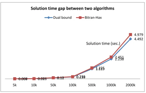
Figure 2.4 The gap of solution time between Bitran-Hax and Dual Bound ... 32

Figure 3.1 Solving Procedure for the ν-SVM ... 50

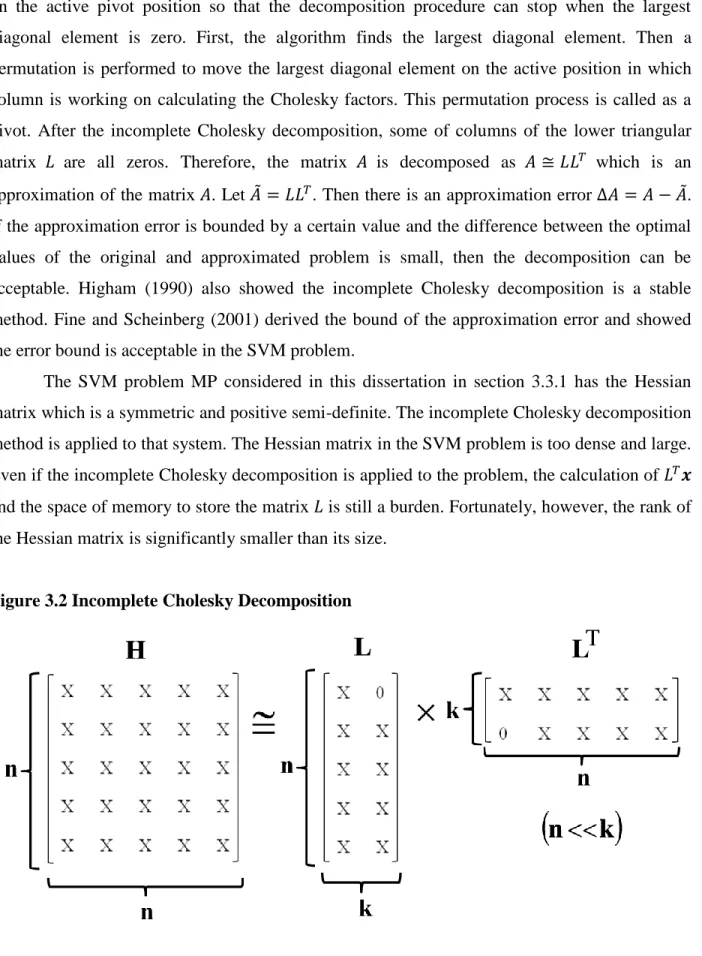
Figure 3.2 Incomplete Cholesky Decomposition... 62

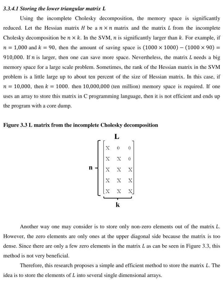
Figure 3.3 L matrix from the incomplete Cholesky decomposition ... 66

Figure 3.4 The method of storing L matrix... 67

Figure 4.1 Supplier Selection Procedure ... 86

Figure 4.2 Solution Procedure for Supplier Selection ... 87

Figure 4.3 Example of a Supplier Selection Problem ... 88

(10)

List of Tables

Table 2.1 Problem size (500,000 variables) ... 30

Table 2.2 Problem size (1,000,000 variables) ... 31

Table 2.3 Problem size (2,000,000 variables) ... 31

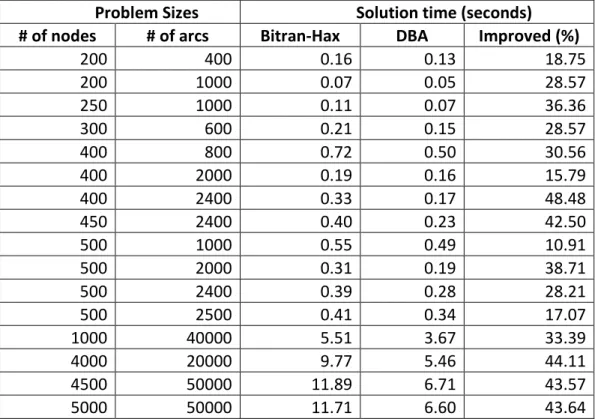
Table 2.4 Computational Results for Quadratic Network Problems ... 33

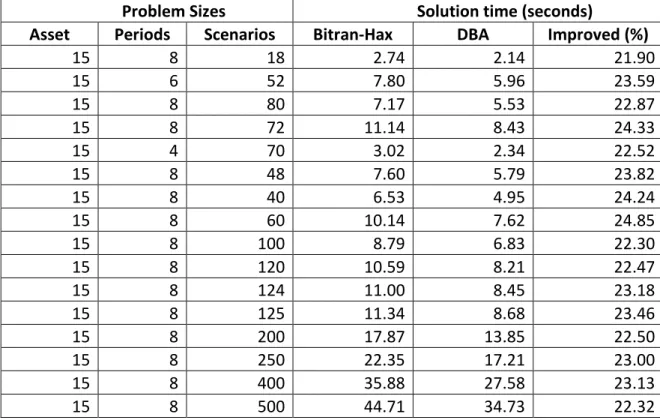
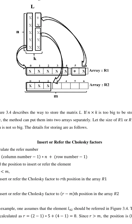
Table 2.5 Computational Results for the Portfolio Optimization Problems ... 34

Table 3.1 SPGM method... 70

Table 3.2 GVPM method ... 71

Table 3.3 MSM method ... 71

Table 3.4 AA method ... 71

Table 3.5 Large-scale problems (MSM method) ... 72

Table 3.6 Large-scale problems (AA method) ... 72

Table 3.7 Sensitivity Analysis of ν for svmguide1 (GVPM method) ... 72

Table 3.8 Sensitivity Analysis of ν for mushrooms (GVPM method) ... 73

Table 3.9 Comparisons of Bitran-Hax and Dual Bound algorithm (AA method) ... 73

Table 4.1 Supply Chain Management with SVM ... 85

Table 4.2 Property of Data Set ... 93

Table 4.3 Experimental Results of Pre-selection using SVM ... 94

Table 5.1 Financial Ratios ... 98

Table 5.2 Classification of credit ratings into good (A~B) and bad (C~D) groups ... 98

(11)

Acknowledgements

I would like to express my deep-felt and sincere gratitude to my advisor, Dr. John Wu. Throughout my research in PhD program at Kansas State University, he provided sound advice, encouragement, thoughtful guidance, lots of good ideas. His broad knowledge and logical way of thinking have been of great value for me. I could not have done my dissertation without his help.

I am deeply grateful to my other advisory committee members: Dr. Todd Easton, Dr. B. Terry Beck, and Dr. Chwen Sheu, for their detailed and constructive comments. I wish to specially thank to Dr. Orlen Grunewald for being my final examination outside chairperson.

I wish to warmly thank Dr. Bradley A. Kramer, Dr. E. Stanley Lee, Dr. David Ben-Arieh, Dr. Shing I. Chang for their valuable encouragement and comments.

I am grateful to the department of Industrial & Manufacturing Systems Engineering for giving me the opportunities, resources, and financial support to finish my research.

I owe my most loving thanks to my wife Mijung Lee, my daughters Youngji and Youngsuh for their loving support, encouragement, and understanding during this work. I also deeply thank my families in Korea for their constant support, encouragement, and advice.

(12)

Dedication

(13)

CHAPTER 1 - Introduction

1.1 Introduction

In real world applications, many decision problems have to be solved in daily operations. Among them, classification is one of important class of decision problems. One may need to classify the things that they did for a day as value added and non-value added tasks. Marketing team may classify the company's markets into several different tiers or segments using pre-defined criteria or performance metrics. Companies may classify their clients into important customers and normal ones in terms of value added contributions to the company's revenue. Companies may classify their suppliers into qualified or potential supplier groups based on various supplier evaluation criteria. Countries may classify other countries into friendly-nations (allies) and the others. When one makes a decision for any classification problem, intuitive solutions to any classification problem are easy and simple. However, such solutions are sometimes wrong because the decisions are too subjective. To avoid this happening, researchers have suggested a variety of systematic methods for making decisions about problems in classification.

One good scientific method for classification problems is the machine learning method in the field of data mining (Vapnik, 1995). The classification problem is sometimes referred as the pattern recognition problem. The support vector machine is a machine learning tool for regression and classification problems. This dissertation focuses on the development of a solution algorithm for the support vector machine (SVM) and its applications. Compared with other statistical methods, the SVM does not require any parameters. Thus, the SVM is sometimes called a non-parametric method. Moreover, the SVM can handle large-scale problems. Before the SVM methods were proposed in 1995, machine learning method using neural networks are the popular approaches for attacking classification problems. The neural network had two main drawbacks of the generalization and the slow convergence because the performance of the neural networks is data dependent and the method consumes a lot of memory and processing time to run. The SVM has overcome these drawbacks in both theoretical and practical aspects.

In this research, an efficient solution approach for the SVM is proposed using symmetric kernel method. The method consists of the matrix splitting method, the gradient projection

(14)

method, and the incomplete Cholesky decomposition. The proposed method enables us to use several options for both the line search and updating parameters.

In addition, this research proposes a solution algorithm for the subproblem of the SVM and suggests an efficient solution procedure of the supplier selection problem using the SVM. In solving a classification problem using SVM, a quadratic knapsack subproblem needs to be solved repeatedly and they are frequently the most time consuming task in the solution processes. A new pegging algorithm is proposed for solving the nonlinear knapsack subporblem arising in the SVM. This newly proposed method for solving the continuous nonlinear knapsack problem can significantly reduce the time consuming steps in the solution processes.

For applications to the classification problems using SVM, an efficient integrated solution method is suggested for the supplier selection problem. The selection of qualified suppliers is an important issue for many companies because it directly affects the quality of products as well as the potential profits. The SVM can classify suppliers into two groups such as the qualified suppliers and the potential suppliers. The final suppliers out of potential suppliers are then selected based on other considerations such as the requirements products, due dates, consolidations, and final costs. In section 2, the motivation of this research is described. The contribution of this dissertation is presented in section 3. An overview of this dissertation is in section 4.

1.2 Research Motivations

The motivation of this research started with the technical issues that arise in the SVM. The SVM has been a popular machine learning method for about fifteen years now since many studies (Bennett and Bredensteiner (1997), Suykens and Vandewalle (1999), Joachims (1999), Platt (1999), Crisp and Burges (2000), Bennett and Bredensteiner (2000), Lee and Mangasarian (2001), To et al. (2001), Zhou et al. (2002), Zhan and Shen (2005), Bach and Jordan (2005), Kianmehr and Alhajj (2006), Mavroforakis and Theodoridis (2006), An et al. (2007), Alzate and Suykens (2008)) have proved that the SVM is an efficient method both theoretically and practically. Given its popularity, three types of major studies have focused on its use: formulation, solving algorithm, and applications. One recent formulation of the SVM is the -SVM, which is less sensitive to a regularization parameter than -SVM (Nehate, 2006). This research focused on the -SVM. Most solving algorithms for the SVM have been proposed by

(15)

using -SVM formulation. For large-scale data sets, the working set or the sequential minimal optimization (SMO) type method is the only one that can solve problems. Other methods have worked with small to medium sized problems. This motivated us to develop an efficient solving algorithm for the -SVM for the typically large-scale classification problem using non-SMO type methods. The advantage of the non-SMO type method is to use more algorithms that have been already developed for quadratic or nonlinear programming problems. Some attempts have used the non-SMO type method, but the size of the data set has been a major limitation. Therefore, this research proposes a non-SMO type solution method for the -SVM classification problem.

To solve the -SVM classification problem, a quadratic programming problem must be solved. This problem has a quadratic objective function with a dense Hessian matrix, a single linear constraint, and box constraints. The proposed solving algorithm in my research is an iterative method. At each iteration, a subproblem with continuous quadratic objective function and knapsack constraint needs to be solved which frequently is the most time consuming step in the solution processes. If one can improve the algorithm to solve the continuous quadratic knapsack problem, the SVM problem itself can be solved more efficiently. This motivates the development of a new pegging algorithm for the continuous nonlinear knapsack problem. The Bitran-Hax (1981) algorithm is the pegging algorithm used for the continuous nonlinear knapsack problem. However, this research found that the Bitran-Hax algorithm has two time consuming calculations at each iteration. First is the recalculation of the primal solutions after each dual iteration and check their feasibilities. The other time consuming calculation is to calculate the dual solution at each iteration. These two challenging issues are the main motivation for the development of the dual bound pegging algorithm.

This research finally focuses on applying SVM. Many applications exist for the -SVM classification problem. This research focuses on the supplier selection problem in supply chain management (SCM). If a company selects non-qualified suppliers, then the quality of the product could be out-of-controlled and the on time deliveries may not be fulfilled at the desired level. This could very likely have significant impact the company's ultimate profit and reputation. Therefore, the supplier selection problem is an important issue in many companies. If a company can find a more efficient and accurate method for selecting suppliers, then the company could easily gain more profits or market shares, which are the goals of most for-profit companies. This

(16)

issue motivated us to propose an efficient solution approach for the supplier selection problem. It is well-known that the supervised machine learning method is frequently more accurate and more efficient than the unsupervised method through existing literatures. This research used the SVM as a supervised machine learning method for selecting potential suppliers from all suppliers considered. In case of that there exist the past data for the supplier selection of a company, the SVM can solve the supplier selection problem better than unsupervised method. Another application of SVM to financial area is the company credit ratings. Credit rating is a very important factor for investing or loan to companies and also significant measurement of the company. This research applies the newly proposed SVM algorithm to predict credit ratings of companies in Korea.

1.3 Research Contributions

This research combines three major topics: mathematical programming, data mining, and supply chain management. Therefore, the contributions of the research range from theoretical to practical. One of the theoretical contributions is the development of a new pegging algorithm for solving the continuous nonlinear knapsack problem. Another theoretical contribution is to propose an efficient solving method for the -SVM classification problem. The practical contribution in this research is to suggest a new integrated solving approach for the supplier selection problem.

The Bitran-Hax algorithm is a famous pegging algorithm for the continuous nonlinear knapsack problem. The algorithm is known to be simple and fast. This research aims to improve on the Bitran-Hax algorithm. This research found that the algorithm does two time consuming calculations at each iteration. These two tasks are the calculation of a dual solution and those of the primal variables. The dual solution is calculated by the summation of the gradient of the functions at each iteration. The new algorithm splits this calculation and reduces re-calculations. Calculating primal variables is simple, but must be done for all free variables at each iteration. The new algorithm uses a dual variable instead of all free primal variables. The reason the Bitran-Hax algorithm calculates primal variables at each iteration is to check the feasibility of each variable. The main idea of the new algorithm is to use the bounds of the dual variable instead of the primal variables to check the feasibilities. The contributions of solving the continuous nonlinear knapsack problem are as follows.

(17)

 This research developed a new pegging algorithm for the continuous nonlinear knapsack problem.

 The new algorithm has two advantages: it removes the calculations of primal variables at each iteration and updates the dual solution instead of re-calculating.

 The solution time of the new algorithm is overall faster than the Bitran-Hax algorithm.  The new algorithm is faster when the size of the problem is large.

The -SVM classification problem has a quadratic objective function, two linear constraints, and box constraints. First, this research gets one of linear constraints on the objective function using the augmented Lagrangian method. Then the problem becomes a singly linearly constrained quadratic convex programming problem. The Hessian matrix is a dense positive semi-definite matrix. The proposed method in this research splits the dense positive semi-definite Hessian matrix as the sum of two matrices. The algorithm solves a subproblem with a simple diagonal Hessian matrix, one of these two matrices, and can choose the Hessian matrix for the subproblem with any simple and nonsingular matrix. The subproblem is a continuous quadratic knapsack problem and can be solved by the new method proposed in this research. The current solution and the solution of the subproblem are used for calculating the direction vector. In the next step, the line search is conducted to find the best step size. Then the algorithm updates solutions and a parameter. In the line search and updating parameter steps, the algorithm can take advantage of several options like monotone or nonmonotone line search for the line search and Barzilai & Borwein (BB) (1988) rule for updating a parameter. Even if the algorithm splits the Hessian matrix, there are a few steps to calculate the Hessian matrix. To facilitate the calculation, the incomplete Cholesky decomposition method is applied to decompose the Hessian matrix if kernel method is applied. The contributions for the -SVM classification problem can be summarized as follows:

 This research proposes a different approach for solving -SVM classification.

 The method is a combination of matrix splitting, gradient projection, and incomplete Cholesky decomposition.

 The subproblem can be solved with an efficient solving algorithm such as dual bound algorithm.

(18)

The supplier selection problem is an important issue for a company purchasing raw materials or some components for production from other companies. In the supplier selection problem, three major issues contribute the decision: the definition of criteria, the quantification of the criteria, and the selection method for potential suppliers and final suppliers. This research focuses on the method for selecting suppliers. Most methods for selecting suppliers do not need historical data for the selection. These methods use and check only the suppliers currently considered. This method is the unsupervised method. On the other hand, if a company has historical data for selecting suppliers, a supervised method like the SVM can be used. It is well known the supervised method is more accurate than the unsupervised method. The main idea of this research is to use SVM classification for selecting potential suppliers. The potential supplier denotes a supplier eligible to contract with a company. The company selects the final suppliers out of all potential suppliers. The potential suppliers can be considered the candidates for final suppliers. Selecting potential suppliers is a classification problem, and the SVM classification can be applied. To select the final suppliers, this research used a mixed integer programming model. The summary of the contribution of the supplier selection problem is as follows:

 This research suggests an integrated solving approach for the supplier selection problem.

 The SVM classification is used to select potential suppliers.

 A supervised method like the SVM is more accurate than an unsupervised method.  The proposed method is simpler than other methods.

In the last part of this research, it applies the proposed method of SVM to a financial problem. Banks or investment companies want to measure eligible companies with appropriate and objective criteria. One well-known measurement is the company credit rating. The ratings are A through D. This research classifies companies into qualified company and others using SVM. Experimental results show that the newly proposed SVM solution method is good potential method for predicting the company credit ratings.

(19)

1.4 Dissertation Overview

In Chapter 2 of this dissertation, it describes the development of a new pegging algorithm for the continuous nonlinear knapsack problem introducing the new concept of the dual bound. The algorithm is compared with the Bitran-Hax algorithm because the new algorithm is an extension of the Bitran-Hax algorithm. Experimental results are shown as well.

In Chapter 3, the solution method for -SVM classification problem is presented. This research describes the history of SVM problems first and solving algorithms. Then, it proposes a method consisting of several mathematical methods. The incomplete Cholesky decomposition method and an efficient data storage method for a large scale lower triangular matrix are introduced. Some options for the line search and the parameter updating method are shown with some experimental results.

In Chapter 4, the supplier selection problem is described. The integrated solving approach for the supplier selection problem combines the SVM classification method with mathematical programming model for selecting suppliers. To compare with the SVM classification method, the analytic hierarchy process (AHP) for selecting potential suppliers is described. A mixed integer programming model is presented for selecting the final suppliers from the potential suppliers.

In Chapter 5, an application of financial problem using SVM is presented with the prediction of company credit ratings with real company data. The overall conclusion and future work of this research will be in the last Chapter 6.

(20)

CHAPTER 2 - Continuous Nonlinear Knapsack Problem

In this chapter, this research proposes an efficient pegging algorithm for solving continuous nonlinear knapsack problems with box constraints. The problem is to minimize a convex and differentiable nonlinear function with one equality constraint and bounds on the variables. One of the main approaches for solving this problem is the variable pegging method. The Bitran-Hax algorithm is a well-known pegging algorithm that has been shown to be a preferred choice especially when dealing with large-scale problems. However, it needs to calculate an optimal dual variable and update all free primal variables at each iteration, which frequently is the most time-consuming task. This research proposed a Dual Bound algorithm that checks the box constraints implicitly using the bounds on the Lagrange multiplier without explicitly calculating primal variables at each iteration and updating the dual solution in a more efficient manner. The results from the computational experiments have shown that the proposed new algorithm constantly outperforms the Bitran-Hax algorithm in all the baseline testing and two real-time application models. The proposed algorithm shows significant potentials to be used in practice for many other mathematical models in real-world applications with straight-forward extensions.

2.1 Introduction

The knapsack problem, also known as the resource allocation problem, is that a hitchhiker wants to pack his knapsack by selecting from among various possible objects those which give him maximum comfort, which can be formulated by a mathematical model with the objective function is to maximize the total comfort, one knapsack constraint of the capacity of knapsack, and binary variables which are defined in Martello and Toth, (1980).

If its objective function is nonlinear, then the problem is a nonlinear knapsack problem. There are some classes of the nonlinear knapsack problem and the review of these can be found in Bretthauer and Shetty, (2002). This research is interested in the problem which has a convex, differentiable, and nonlinear objective function, and box constraints for all variables, which is a convex, separable, and continuous type of problem. There are many applications for problems of this type which is described in Robinson et al. (1992) such as portfolio selection problem in Markowitz (1952), multi-commodity network flow problem Ali et al. (1980), transportation

(21)

problem in Ohuchi and Kaji (1984), support vector machine in Nehate (2006), production planning in Tamir (1980), and convex quadratic programming in Dussault et al. (1986). The problem also can be considered as a subproblem for many optimization models. Ibaraki and Katoh (1988) discussed comprehensively the algorithmic aspects of resource allocation problem and its variants in their book. Twenty years later, Patriksson (2008) surveyed the history and applications of the problem as well as solving algorithms. Therefore these literatures are not reviewed here.

This research considers a continuous nonlinear knapsack problem with box constraints as follows.

(P1) (2.1)

(2.2)

(2.3)

where is a nonlinear, convex, and differentiable function, is linear referred as the knapsack constraint in the rest of the thesis, for all , and this research assumes all coefficients of are not zero and

and is invertible.

The Lagrangian dual formulation of P1 by relaxing the knapsack constraint (2.2) is as follows.

(D1) (2.4)

where (2.5) (2.6) and is the Lagrange multiplier corresponding to the knapsack constraint (2.2).

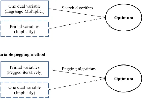
The nonlinear knapsack problem P1 is frequently solved via an iterative manner. There are more than a handful of algorithms proposed to solve this problem and they can be generally divided into two main categories (Patriksson, 2008): the Lagrange multiplier search method and the variable pegging method. The basic ideas of these two methods are in the following pictures.

(22)

Figure 2.1 Lagrange multiplier search method

Figure 2.2 Variable pegging method

In Figure 2.1 and 2.2, solid boxes denote a variable or variables explicitly used to find the optimal solution in each algorithm and dashed boxes represent a variable or variables implicitly optimized as the other variable or variables are explicitly optimized. As Bretthauer and Shetty (2002) mentioned in their paper, while the Lagrange multiplier search method maintains all Karush-Kuhn-Tucker (KKT) conditions during its iterations, except the one knapsack constraint and its corresponding complementary slackness condition, the pegging method maintains all KKT conditions during its iterations except box constraints. That means the multiplier search method focuses on one dual variable achieving the optimal point, and the pegging method aims to find the optimal solution satisfying the feasibility of all primal variables. In Figure 2.1, the Lagrange multiplier search method uses the dual variable to find the optimal dual solution using a search algorithm because there is only one dual variable in the dual problem D1 which is described in Bazaraa et. al (1993) and Martello & Toth (1990). As the dual variable is optimized, the corresponding primal variables are implicitly optimized as well. On the other hand, in Figure 2.2, the variable pegging method is a type of primal algorithm finds the optimal primal solution by pegging some variables to their lower or upper bounds as their optimal value each iteration. In this algorithm, the dual variable can be also optimized implicitly as well. In his literature review,

(23)

Patriksson (2008) did not make clear which approach was better in terms of computational complexity or average solution time. The biggest drawback of the pegging algorithm is that the relaxed problem should have an optimal solution and its efficiency depends on whether the optimal solution of the relaxed problem can be obtained in closed form. However, the pegging algorithm requires the objective function to be convex at least for the linear explicit constraints convergence of the method while the multiplier search method requires the objective function to be strictly convex (Patriksson 2008). In addition, Bretthauer et al. (2003) mentioned that the pegging algorithm was typically faster than the multiplier search algorithm when the relaxed subproblem can be solved in closed form. This research focuses on the pegging method since it has nicer finite convergence properties and has good potential to be streamlined for great performances.

The pegging method utilized a relaxed problem of P1 by ignoring the box constraints in (2.3), which has an optimal solution and the corresponding Lagrange multiplier can be solved in a closed form. This relaxed problem can be used to develop an efficient procedure to improve the solution efficiency. In addition, the pegging method generally guarantees a finite convergence. One of the well-known pegging methods is the Bitran-Hax algorithm (1981). Bitran and Hax (1981) developed the algorithm for solving continuous knapsack problem with a convex separable objective function and the coefficients of the equality constraints in (2.2) are ones. The Bitran-Hax algorithm has some very attractive features including the excellent convergence behavior, easy to implement and generally very efficient. There have been many extensions of this algorithm and the reviews of them are referred to (Patriksson, 2008).

In their research, Bitran and Hax (1981) introduced various resource allocation problems that could be formulated with this type of P1 problem. Patriksson (2008) referred to many extensions of this algorithm and reviews them.

Cottle at al. (1986) applied this algorithm to the constrained matrix problem. Eu (1991) formulated the sampling resource allocation problem with the nonlinear knapsack problem and solved the problem with the Bitran-Hax algorithm. Bretthauer et al. (1999) also studied the stratified sampling problem with integer variables, which was solved by the branch and bound algorithm for the main problem and the variable pegging algorithm for its subproblem.

(24)

Extensions have been applied to more general problems. Ventura (1991) extended the Bitran-Hax algorithm to a problem with non-unit coefficients in the knapsack constraint. Kodialam and Luss (1998) developed the algorithm to solve a nonlinear knapsack problem with non-negativity constraints on variables and a nonlinear convex knapsack constraint. The RELAX algorithm they proposed only checks the lower bound for pegging. Bretthauer and Shetty (2002) proposed a pegging branch and bound algorithm for more general problems with integer variables and a nonlinear convex objective function and knapsack constraint. Bretthauer et al. (2003) extended the pegging branch and bound algorithm to problems with additional block diagonal constraints.

Using the relationship between the restricted projection problem and the nonlinear knapsack problem, a projected pegging algorithm has been proposed. Robinson et al. (1992) introduced a pegging algorithm incorporated with the restricted projection method. If the objective function is the sum of squared variables and there are one linear knapsack constraint and box constraints, then the problem is equivalent to a problem finding the orthogonal projection of the origin on the feasible region. Robinson et al. (1992) used this projection method in the pegging algorithm to calculate the primal solutions of a relaxed problem with only the knapsack constraint and then checked the box constraints. Stefanov (2004) considered a problem with the objective function as a sum of squared subtraction of two variables and also used the concept of projection in the pegging algorithm and extended the algorithm that considered the case of some zero coefficients in the knapsack constraint.

As the literature shows, most extensions of the pegging algorithm focused on improving the calculation of the primal solution of the relaxed problem. On the other hand, the new algorithm in this research does not use the primal solutions of the relaxed problem, using instead the dual bound to check bound constraints.

This research presents another extension of the Bitran-Hax algorithm. Based on the preliminary computational experiments, this research discovered the efficiency of the Bitran-Hax algorithm suffers from two time consuming tasks. Firstly, in the Bitran-Hax algorithm, all primal free variables have to be recalculated at each iteration, where a free variable means the unpegged variable. Secondly, in the Bitran-Hax algorithm, the dual variable, , must be searched and reevaluated several times to determine its optimal value. These are usually the two most time

(25)

consuming procedures in the algorithm and they are the main motivations of this research. In the Bitran-Hax, the algorithm checks the feasibility of the solution after it solves the relaxed problem by ignoring the box constraints in (2.3) at each iteration. Solving the relaxed problem is the calculation of a newly trial dual variable at each iteration. Then, the algorithm calculates the primal variables again and then rechecks their box constraints for the feasibility. Basically, the newly proposed algorithm establishes a set of bounds as the predicted range of the optimal dual solution, which can be defined initially using only the input data. This is then used as the criterion for feasibility instead of checking the feasibility of the primal variables at each iteration. The dual bound is calculated only once initially and need not be updated during the solution process. For calculating the optimal dual solution, the new algorithm divides the calculations of the dual variables into several smaller components, and just updating the required components during the pegging process.

The objective of this chapter is to develop a new pegging algorithm based on the concepts of the Bitran-Hax algorithm to solve the continuous separable nonlinear knapsack problem with one linear equality knapsack constraint and box constraints. In the newly proposed algorithm, the new algorithm introduces the concept of the dual bound and how the dual bound can speed up the solution process. The computational results on randomly generated problems and applications embedded test models show that the new algorithm consistently outperforms the Bitran-Hax algorithm.

In the rest of the chapter, the concept of the Bitran-Hax algorithm as a current state-of-the-art pegging method is described in section 2. The new pegging algorithm for continuous nonlinear knapsack problem is presented in section 3. The new algorithm applies to the continuous quadratic knapsack problem as a special case of the nonlinear knapsack problem and the experimental results are shown in section 4. In the conclusion, the contributions of this research are reviewed.

(26)

2.2 The Bitran-Hax algorithm

This section presents the Bitran-Hax Algorithm to solve the problem P1. The problem P1 is a convex problem with linear constraints, so the following Karush-Kuhn-Turker (KKT) conditions are necessary and sufficient for the optimality as described in Mangasarian (1969). The Karush-Kuhn-Turker (KKT) conditions of the problem P1 are

, for all (2.7) , for all (2.8) , for all (2.9) , (2.10) , for all (2.11) , for all (2.12)

where is the Lagrange multiplier for the knapsack constraint (2.2), and , for all are the Lagrange multiplier for the lower and upper bounds in (2.3), respectively.

If one relaxed the box constraint in (2.3) in the problem P1, the equation (2.7) becomes , for all and and can be solved in closed form. Since is linear, its gradient is merely a constant defined as . Assuming , for all , is invertible, can be calculated as,

_{, for all} _(2.13) where denotes the inverse of , the gradient of objective function , and the Lagrange multiplier corresponding to the knapsack constraint in (2.2) can be obtained from the KKT conditions of P1 without the box constraints

(2.14)

If the solution in (2.13) satisfies the box constraints (2.3) in P1, then it is also optimal to P1. If not, then one can set for some to their upper or lower bounds and then the value of can be recalculated. To determine which variables are to be fixed at their bounds, one defines following two terms as the sums of over and under limits, respectively.

(27)

Q , where (2.16) where is defined in (2.13). and are used for choosing which set of variables (variables in and ) to be pegged in the algorithm. The following theorem describes how to choose the pegging variables.

Theorem 2.2.1

, for all (2.17) , for all (2.18) , for all (2.19) , for all , , for all (2.20) where is the optimal solution of the problem P1.

Proof

This theorem can be proved using Bitran and Hax's (1981) work. The proof uses the KKT condition of the problem (P1). The Lemma 1, Lemma 2, Theorem 1, and Theorem 2 in Bitran and Hax (1981) described that each case of and in (2.17) ~ (2.20) is related with the inequalities among the first derivatives , for all i=1,…,n (See details in Bitran and Hax (1981)). Using this result and the KKT condition, Theorem 3 in their paper showed that setting the optimal value at each case at the upper bound or the lower bound or the optimal value as obtained by (2.13) in the relaxed problem is optimal in the original problem (P1). Ventura (1992) also showed the relationship of these cases at Theorem 6 in his paper.

The related computational experiments can be found in Wu (1993). The detail steps of Bitran-Hax algorithm are as follows.

Bitran-Hax Algorithm Step 0 (Initialization)

Let , , Step 1 (Calculating Dual Solution and Primal Solution)

(28)

Compute ,

Calculate _{for all} Step 2 (Check feasibility)

For all .

If for all , then it is optimal and go to Step 6. Otherwise, go to Step 3.

Step 3 (Calculate Pegging Sums & Check Stopping Criterion) Compute and

, where . Q , where . If and are empty,

then it is optimal and calculate for all from (13) and go to Step 6. Step 4 (Pegging Variables)

If , then

set for all ,

let _and

. If , then

set for all ,

let _and

. If , then

set for all , set for all , let _and

. Step 5 (Check Stopping Criterion)

(29)

Else, set and go to Step 1. Step 6 (Optimum Found)

Set for all as the optimal solution and terminate.

The Bitran-Hax Algorithm guarantees that at least one variable is pegged (or fixed) at each iteration since if there is no variable to be pegged at the current iteration, then the current solution on hand is optimal. Therefore, the algorithm can reduce the dimension of the problem as it progresses, and thus, guarantee the finite convergence. For the solution time, Wu (1993) has shown that the Bitran-Hax algorithm outperforms the Helgason et al.'s sequential line search and the random search by 25%~48% for quadratic network flow problems. It is, however, significantly slower than these two methods during the later stage of the solution process. With these empirical insights, this research has discovered several unnecessary procedures in the Bitran-Hax algorithm, which means the algorithm can be further streamlined. The calculation of a dual solution and its corresponding primal free variables at each iteration in Step 1 are the two most time consuming tasks, and these are the main foci to be improved in this research. In the next section, this research will show how to streamline these tasks.

2.3 The Dual Bound Algorithm (DBA)

In this section, a new pegging algorithm for continuous nonlinear knapsack problem with box constraints is proposed. The following a definition and two theorems demonstrate the basic ideas of the new algorithm.

Definition 2.3.1

The dual bound is the set of upper and lower bound of Lagrange multiplier corresponding to the solution of the relaxed problem, where the relaxed problem is the problem P1 ignoring the box constraint in (2.3).

Theorem 2.3.1

, for , from (2.13) is a solution of the relaxed P1 problem if it satisfies its box constraint if and only if is within the dual bound corresponding to the variable as follows: , for , where .

(30)

Proof

The optimal solution of the relaxed P1 problem is , for , from (2.13). If one replaces by _{, then the box constraint of} P1 , for become , for . Hence, the bounds on the Lagrange multiplier according to the box constraint can be described by:

, for .

Conversely, if one solves for _{, then one can get} _{which is the same as bound constraint of the variable}_.

Theorem 2.3.1 provides a novel perspective to check the box constraint in (2.3) using the dual bound and shows that the box constraint in the primal problem can be replaced by the dual bound as defined in Definition 2.3.1. Each primal variable has its box constraint, and it can be transformed into the dual bound corresponding to each . In the knapsack problem, the coefficient of the knapsack constraint in (2.3) denotes the weight of the each item. Therefore, if one of coefficients is zero, then the corresponding does not need to be taken into account the knapsack constraint and it can be fixed to its upper bound, which is the reason this research can assume , for all . As stated in Theorem 2.3.1, the calculation of the dual bound only requires the input values: , and , which are known parameters. This property implies one does not have to update the dual bound at each iteration after it has been calculated initially.

Theorem 2.3.2

The solution , for , obtained from (2.13) is an optimal solution of the problem P1 for a given dual solution to D1, if the following inequality holds true:

. Proof

In the Bitran-Hax algorithm, if the solution obtained from using the equation (2.13) satisfies the box constraints (2.3) of P1, then the solution is also optimal to P1. That is, if

(31)

, for all , then is also the optimal solution of the problem P1. From the Theorem 2.3.1, one can easily replace all inequalities of , for all with the following:

.

Theorem 2.3.2 shows if the dual solution satisfies all the dual bounds, then the current solution is then optimal. The primal solution for all satisfies all box constraints in the Bitran-Hax algorithm is the same that the dual solution satisfies all dual bounds in the new algorithm. From these properties, the new algorithm is called Dual Bound algorithm (DBA). The DBA uses a correction value at each iteration when the algorithm calculates the values of and , so these values are the same as the values in the Bitran-Hax algorithm. Therefore, DBA and Bitran-Hax algorithm select the same variables to be pegged at each iteration. The pseudo-code of the proposed algorithm is now summarized below.

Dual Bound Algorithm (DBA) Step 0 Initialization

Let , , Step 1 Calculating Dual Bounds

For all .

Compute

Calculate and Step 2 Update Dual Variable

Compute

Step 3 Calculate Pegging Sums & Check Stopping Criterion Compute and

(32)

where and is correction value. Let ,

Q ,

where and is correction value. Let ,

If and are empty, then it is optimal,

and calculate for all from (2.13) and go to Step 6. Step 4 Pegging Variables

If , then

set for all ,

let _and

. update , _. If , then

set for all ,

let _and

. update _, _. If , then

set for all , set for all , let _and

. update _, _. Step 5 Check Stopping Criterion

If _{, then go to Step 6.} Else, set and go to Step 2. Step 6 Optimum Found

Set for all is the optimal solution and terminate.

The above proposed DBA has two main potential advantages for improving the solution times: (1) eliminating the calculations of all the primal variables in every iteration and (2)

(33)

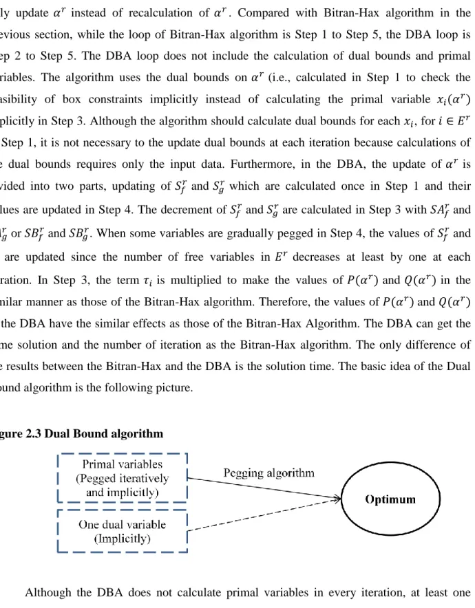
only update instead of recalculation of . Compared with Bitran-Hax algorithm in the previous section, while the loop of Bitran-Hax algorithm is Step 1 to Step 5, the DBA loop is Step 2 to Step 5. The DBA loop does not include the calculation of dual bounds and primal variables. The algorithm uses the dual bounds on (i.e., calculated in Step 1 to check the feasibility of box constraints implicitly instead of calculating the primal variable explicitly in Step 3. Although the algorithm should calculate dual bounds for each , for in Step 1, it is not necessary to the update dual bounds at each iteration because calculations of the dual bounds requires only the input data. Furthermore, in the DBA, the update of is divided into two parts, updating of and which are calculated once in Step 1 and their values are updated in Step 4. The decrement of and are calculated in Step 3 with and or and . When some variables are gradually pegged in Step 4, the values of and are updated since the number of free variables in decreases at least by one at each iteration. In Step 3, the term is multiplied to make the values of and in the similar manner as those of the Bitran-Hax algorithm. Therefore, the values of and in the DBA have the similar effects as those of the Bitran-Hax Algorithm. The DBA can get the same solution and the number of iteration as the Bitran-Hax algorithm. The only difference of the results between the Bitran-Hax and the DBA is the solution time. The basic idea of the Dual Bound algorithm is the following picture.

Figure 2.3 Dual Bound algorithm

Although the DBA does not calculate primal variables in every iteration, at least one primal variable is pegged at each iteration. Therefore, in the DBA, both primal and dual variables are optimized implicitly as illustrated Figure 2.3.

(34)

For the original Bitran-Hax algorithm, in the worst case, only one variable is set to its upper or lower bound at each iteration. The computational complexity of this process is . In addition, there are two calculations of the primal variables and the dual variable at each iteration and the evaluation of the feasibility for all remaining free variables. The computational complexity of this process is . Therefore, the overall computational complexity of the Bitran-Hax algorithm is . In the DBA, the pegging procedure has the same complexity as the Bitran-Hax algorithm and there is the evaluation of the feasibility of all remaining free variables at each iteration of which is the calculation of pegging sums and and its complexity is . The overall computational complexity of the DBA seems to be similar to the Bitran-Hax algorithm. However, except the pegging process, the DBA has only the evaluation of the feasibility process and does not have two calculations of the primal variables and the dual variable. For instance, let us consider the worst case problem that only one variable is pegged at each iteration. In the Bitran-Hax algorithm, the calculation of the primal variables in (2.13) is at each iteration and the overall calculation is the same as the calculation of the sum of to because the number of iteration is (the worst case), that is, . The calculation of the dual variable in (2.14) is also . The total variable updating effort can be as bad as . On the other hand, the DBA only needs to calculate the dual bounds for all variables initially, that is, , but does not need to calculate two . In this respect, it is obvious that the DBA could be more efficient than the Bitran-Hax algorithm unless the problem has only one or two iterations to get the optimum. In the next section, the computational experiments show the practical performance of the DBA.

2.4 Numerical Examples

This section shows the Dual Bound Algorithm for a continuous quadratic knapsack problem as a special case of nonlinear knapsack problem as follows.

(P2) (2.21)

(2.22)

(35)

where for all , and this research assumes for all and .

To simplify the implementation, a variable transformation is first performed to let all the coefficients of the equality constraint become one. This requires the following change of variables.

Let , for all and the bounds become

, for all (2.24) , for all (2.25) The problem is reformulated as

(P3) (2.26)

(2.27)

, for all (2.28) The Karush Kuhn Turker (KKT) conditions of the problem P3 are

, for all (2.29) , for all (2.30) , for all (2.31) , (2.32) , for all (2.33) , for all (2.34)

With this equation, the variable is calculated as follows:

, for all (2.35) where is obtained from the KKT conditions of P2 without the bound constraints

(2.36)

(36)

The equations (2.35) and (2.36) are corresponding to (2.13) and (2.14) respectively. The detail algorithm of Dual Bound is as follows:

Algorithm (Dual Bound : Quadratic Knapsack Problem) Step 0 Initialization

Let , ,

Transform into and compute and for all from (2.24) and (2.25). Step 1 Calculating Dual Bounds

Compute dual bounds for all , for .

Calculate and Step 2 Update Dual Variable

Compute

Step 3 Calculate Pegging Sums & Check Stopping Criterion Compute and , where let , Q , where let ,

If and are empty, then it is optimal,

(37)

Step 4 Pegging Variables Pegging variables

If , then set for all , let _and

. update , _. If , then set for all ,

let _and

. update

, .

If , then set for all , set for all , let _and

. update , _. Step 5 Check Stopping Criterion

If _{, then go to Step 6.} Else, set and go to Step 2. Step 6 Optimum Found

Set for all is the optimal solution and terminate.

In the above algorithm, is the in the previous section. The term in step 3 is the which makes and Q the same as those of Bitran-Hax algorithm. This section provides a simple example to show how the algorithm proposed in this research works. The simple example is solved with the methods of both the Bitran-Hax and the Dual Bound.

Example 4.1

(38)

By the formulation, < Bitran-Hax Algorithm > - Iteration 1 Step 0 , , , , Step 1 Step 2 : Yes : No Step 3

(39)

Step 4 Since , Step 5

Since , set , go to Step 1

- Iteration 2 Step 1 Step 2 : Yes Go to Step 6. Step 6 Set , Therefore, is optimal.

Next, the Dual Bound Algorithm is used to solve this problem. < Dual Bound Algorithm >

- Iteration 1 Step 0

(40)

, , Step 1 Step 2 Step 3 , is empty. Q , , Step 4 Since , Step 5

Since , set , go to Step 2 - Iteration 2

(41)

Step 3 , is empty. Q , is empty. It is optimal. Calculate and go to Step 6. Step 6 Set , Therefore, is optimal.

From this numerical example, two methods have the same optimal solution and the number of iteration. The Bitran-Hax Algorithm calculates and in step 1 at every iteration. On the other hand, The Dual Bound Algorithm calculates dual bounds at the beginning and calculates three components of calculation in step 1. The loop of the Dual Bound Algorithm starts from step 2. The Dual Bound Algorithm does not calculate at every iteration. Furthermore, the Dual Bound Algorithm updates two components of calculation ( , , and ) instead of calculating all it again. In this simple problem, the Dual Bound Algorithm is not much attractive. However, if the size of the problem or the number of iteration is increasing, the solution time would be different. Some experimental results for various large scale problems are shown in the next section.

(42)

2.5 Experimental results

In this section, the computational experiments for both the Dual Bound algorithm (DBA) and the Bitran-Hax algorithm are conducted on randomly generated problems with different sizes, and then tested on different types of applications with common data sets. Both algorithms are implemented in C programming language, complied using gcc and ran on a Fedora 7, 64 bit Red Hat Linux machine with 2 GB memory and Intel Duo CoreTM 2 CPU running 2.66 GHz. Experiments on different types of problems demonstrated a comparison between the Dual Bound and the Bitran-Hax algorithms.

In the first round of tests, the continuous quadratic knapsack test problems with various sizes were randomly generated to establish a baseline comparison between the Bitran-Hax algorithm and the DBA.

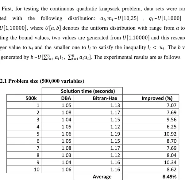
First, for testing the continuous quadratic knapsack problem, data sets were randomly generated with the following distribution: , , and , where denotes the uniform distribution with range from to . For generating the bound values, two values are generated from and this research puts the larger value to and the smaller one to to satisfy the inequality . The value in (22) is generated by . The experimental results are as follows.

Table 2.1 Problem size (500,000 variables)

Solution time (seconds)

500k DBA Bitran-Hax Improved (%)

1 1.05 1.13 7.07 2 1.08 1.17 7.69 3 1.04 1.15 9.56 4 1.05 1.12 6.25 5 1.06 1.19 10.92 6 1.05 1.15 8.70 7 1.08 1.17 7.69 8 1.03 1.12 8.04 9 1.04 1.16 10.34 10 1.06 1.16 8.62 Average 8.49%

(43)

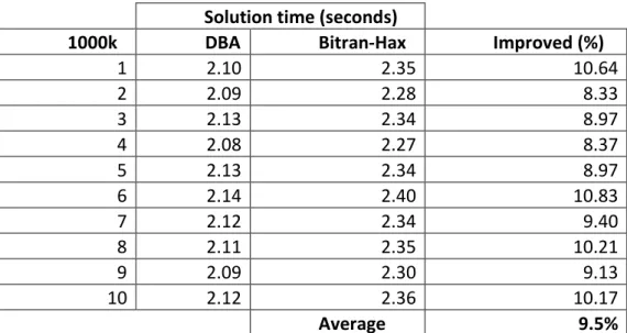
Table 2.2 Problem size (1,000,000 variables)

1 2.10 2.35 10.64 2 2.09 2.28 8.33 3 2.13 2.34 8.97 4 2.08 2.27 8.37 5 2.13 2.34 8.97 6 2.14 2.40 10.83 7 2.12 2.34 9.40 8 2.11 2.35 10.21 9 2.09 2.30 9.13 10 2.12 2.36 10.17 Average 9.5%

Table 2.3 Problem size (2,000,000 variables)

1 4.20 4.61 8.89 2 4.22 4.67 9.63 3 4.20 4.85 13.40 4 4.26 4.66 8.58 5 4.27 4.82 11.41 6 4.26 4.82 11.62 7 4.28 4.83 11.39 8 4.19 4.67 10.28 9 4.26 4.75 10.36 10 4.18 4.68 10.68 Average 10.62%

The experimental results from Tables 2.1 to 2.3 have shown that the DBA outperforms the Bitran-Hax algorithm by 8 ~ 10%. In this set of test problems, around 30~40% of the remaining free variables (i.e., variables having their optimal values strictly between their bounds) are in the optimal solution.

The next set of test problems were randomly generated with the following distributions: , , , and .

(44)

Figure 2.4 The gap of solution time between Bitran-Hax and Dual Bound

In Figure 2.4, the horizontal axis denotes the problem sizes ranging from 5,000 to 2,000,000 variables. From the results illustrated in Figure 2.4, this research discovered that when the problem size increases, the gap of the solution times between the Bitran-Hax and the DBA also increases. When the problem size is small (i.e., ranging from 5,000 to 100,000 variables), the gap of the solution time is small. On the other hand, for the large size problems (i.e., from 500,000 variables and beyond), the gap is large. The percentages of free variables at the achieved optimal solution are about 70% in these test problems. The percentages of free variables at the final optimal solution are larger than the previous experimental results in Tables 2.1~3. However, the improvements on solution times are not much different (i.e., around 8~10% of improvement) because the number of iteration in the results of Figure 2.4 is less than those presented in Tables 2.1~3. Therefore, the DBA outperforms the Bitran-Hax algorithm regardless the number of optimal free variables or required total number of iterations to achieve the optimal solutions.

Second, this research examined the test cases for the some real-world applications having embedded convex knapsack problems in its optimization problems. Two types of optimization problems: quadratic network flow problem and portfolio optimization problem have been tested

0.008 0.018 0.11 0.218 1.119 2.238 4.492 0.007 0.02 0.12 0.239 1.225 2.451 4.979 5k 10k 50k 100k 500k 1000k 2000k

Solution time gap between two algorithms Dual bound Bitran-Hax