Scholarship@Western
Scholarship@Western
Electronic Thesis and Dissertation Repository8-4-2020 1:00 PM
Classification-based method for estimating dynamic treatment
Classification-based method for estimating dynamic treatment
regimes
regimes
Junwei Shen, The University of Western Ontario
Supervisor: He, Wenqing, The University of Western Ontario
A thesis submitted in partial fulfillment of the requirements for the Master of Science degree in Statistics and Actuarial Sciences
© Junwei Shen 2020
Follow this and additional works at: https://ir.lib.uwo.ca/etd
Part of the Biostatistics Commons
Recommended Citation Recommended Citation
Shen, Junwei, "Classification-based method for estimating dynamic treatment regimes" (2020). Electronic Thesis and Dissertation Repository. 7143.
https://ir.lib.uwo.ca/etd/7143
This Dissertation/Thesis is brought to you for free and open access by Scholarship@Western. It has been accepted for inclusion in Electronic Thesis and Dissertation Repository by an authorized administrator of
Dynamic treatment regimes are sequential decision rules dictating how to individualize treatments to patients based on evolving treatments and covariate history. In this thesis, we investigate two methods of estimating dynamic treatment regimes. The first method extends outcome weighted learning from two-treatments to multi-treatments and allows for negative treatment outcome. We show that under two different sets of assumptions, the Fisher consis-tency can be maintained. The second method estimates treatment rules by a neural classifica-tion tree. A weighted squared loss funcclassifica-tion is defined to approximate the indicator funcclassifica-tion to maintain the smoothness. A method of tree reconstruction and pruning is proposed to increase the interpretability. Simulation studies and real application to data from Sequential Treatment Alternatives to Relieve Depression (STAR*D) clinical trial are conducted to illustrate the pro-posed methods.
Keywords: Classification methods, dynamic treatment regimes, neural classification tree, outcome weighted learning, personalized medicine, support vector machine
Traditionally, treatments for patients are decided by clinical judgments based on clinician’s experience or practice guidelines based on clinical evidence and expert opinions. Patients with the same disease often receive the same treatment. It is one-size-fits-all approach. However, patient heterogeneity makes it possible that the best treatment for one patient is suboptimal for another. Therefore, it is important to make an transition from the traditional one-size-fits-all approach to individualized treatment rule which takes personal characteristics into account and tailors treatments to patients. This thesis will present two methods of identifying individualized treatment rule, called multicategory outcome weighted learning and neural classification tree.
I would like to convey my profound gratitude to my supervisor, Dr. Wenqing He, for his scientific guidance, support and for sharing his expertise throughout my study at Western. This thesis would not have been possible without his insights and helpful comments.
I would like to express my thanks to Dr. Grace Yi. The data science meetings arranged by Dr. Yi and Dr. He deepened my interests in statistics and exposed me to the cutting-edge research problems.
I would like to thank my thesis examiners, Dr. Yun-Hee Choi, Dr. Cristian Bravo Roman, Dr. Jiandong Ren for taking the time to read my thesis and for the helpful comments.
Last but not least, I would like to thank my family and my friends at Western for their love and encouragement. The study and life at Western would not have been such happy without their constant support.
Contents
Abstract i
Lay Summary ii
Acknowledgements iii
List of Figures vii
List of Tables viii
1 Introduction 1
1.1 Dynamic treatment regimes . . . 1
1.2 Potential outcomes framework . . . 4
1.3 Review of reinforcement learning . . . 6
1.4 Review of indirect methods . . . 7
1.4.1 Q-learning . . . 8
1.4.2 G-estimation in structural nested mean model . . . 10
1.5 Review of direct methods . . . 12
1.5.1 Inverse probability weighting . . . 12
1.5.2 Outcome weighted learning . . . 14
1.6 Objectives and organization . . . 16
2 Multicategory Outcome Weighted Learning 18 2.1 Introduction . . . 18
2.3 Method framework . . . 21 2.3.1 Single stage . . . 21 2.3.1.1 Fisher consistency . . . 23 2.3.1.2 Computation details . . . 25 2.3.2 Multi-stage . . . 33 2.4 Numerical investigation . . . 34 2.4.1 Simulation study . . . 34
2.4.2 Application to STAR∗D study . . . 41
2.5 Conclusion . . . 43
2.6 Appendix . . . 44
3 Dynamic Treatment Regimes based on Neural Classification Tree 47 3.1 Introduction . . . 47
3.2 Literature review . . . 48
3.2.1 Neural network . . . 48
3.2.2 Classification tree . . . 49
3.3 Neural network architecture for the DTR . . . 51
3.4 Tree reconstruction and pruning . . . 55
3.5 Numerical investigation . . . 57
3.5.1 Simulation study . . . 57
3.5.2 Application to STAR∗D study . . . 63
3.6 Conclusion . . . 64
4 Conclusion 66
Bibliography 69
A R Functions for First Model 73
Curriculum Vitae 117
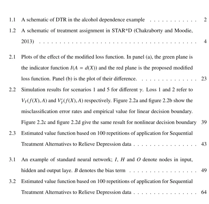
1.1 A schematic of DTR in the alcohol dependence example . . . 2 1.2 A schematic of treatment assignment in STAR*D (Chakraborty and Moodie,
2013) . . . 4 2.1 Plots of the effect of the modified loss function. In panel (a), the green plane is
the indicator functionI(A = d(X)) and the red plane is the proposed modified loss function. Panel (b) is the plot of their difference. . . 23 2.2 Simulation results for scenarios 1 and 5 for differentγ. Loss 1 and 2 refer to
VY(f(X),A) andVYc(f(X),A) respectively. Figure 2.2a and figure 2.2b show the
misclassification error rates and empirical value for linear decision boundary. Figure 2.2c and figure 2.2d give the same result for nonlinear decision boundary 39 2.3 Estimated value function based on 100 repetitions of application for Sequential
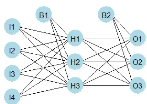
Treatment Alternatives to Relieve Depression data . . . 43 3.1 An example of standard neural network; I, H and O denote nodes in input,
hidden and output laye. Bdenotes the bias term . . . 49 3.2 Estimated value function based on 100 repetitions of application for Sequential
Treatment Alternatives to Relieve Depression data . . . 64
List of Tables
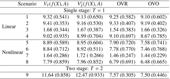
2.1 Misclassification error rates approximated by validation data set of size 1000, averaged over 500 simulation runs; the numbers in parenthesis are standard deviations over 500 simulation runs . . . 40 2.2 Empirical value function approximated by validation data set of size 1000,
av-eraged over 500 simulation runs; the numbers in parenthesis are standard devi-ations over 500 simulation runs . . . 41 3.1 Misclassification error rates approximated by validation data set of size 1750,
averaged over 500 simulation runs; the numbers in parenthesis are standard deviations over 500 simulation runs . . . 62 3.2 Empirical value function approximated by validation data set of size 1750,
av-eraged over 500 simulation runs; the numbers in parenthesis are standard devi-ations over 500 simulation runs . . . 62
Introduction
1.1
Dynamic treatment regimes
Personalized medicine is a medical paradigm where treatment is customized for each patient based on individual information. The motivation behind this paradigm is the fact that het-erogeneity exists among different patients and when making medical decisions, the existing heterogeneity needs to be taken into account. For example, patients may respond differently to the same drug because of their personal difference. In this case, without considering personal information, the one-size-fits-all approach will result in inefficient or over treatment. Dynamic treatment regimes (DTR), also known as adaptive treatment strategies, generalize personal-ized medicine to time-varying treatment settings in which treatment is repeatedly tailored to a patient’s dynamic state (Chakraborty and Murphy, 2014).
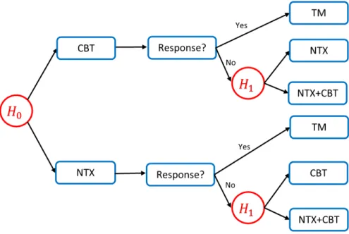
A simple example of dynamic treatment regimes is the treatment of alcohol dependence (Chakraborty and Moodie, 2013). Two stages are involved: initially, clinician prescribes either naltrexone (NTX) or cognitive behavioral therapy (CBT) to the patients. Patients are then classified as responder or non-responder based on the number of heavy-drinking days within the next two months after they take the initial treatment. If a patient experiences more than two heavy-drinking days during the following two months, the patient is labelled as a
responder, otherwise a responder. At the second stage, the non-responders to NTX will be assigned either CBT or an augmentation of NTX with CBT and the non-responders to CBT will be assigned either NTX or an augmentation of CBT with NTX. All responders will receive telephone monitoring (TM) within the next six months.
Figure 1.1 gives a schematic of a possible DTR in the alcohol dependence example. This DTR consists of two decision rules: the first decision rule prescribes the initial treatment based on the baseline information H0 and the second decision rule use intermediate outcome and
updated informationH1to assign the secondary treatment. Specifically, the DTR is: at the first
stage, prescribe CBT if the baseline level of some variable exceeds the pre-specified threshold and otherwise prescribe NTX; at the second stage, if a patient is a responder to the initial treatment, prescribe TM as the secondary treatment; if a patient is a non-responder, switch to the other treatment or prescribe an augmentation based on whether the intermediate level of some variable exceeds the pre-specified threshold.
Figure 1.1: A schematic of DTR in the alcohol dependence example
Another example is Sequential Treatment Alternatives to Relieve Depression (STAR*D) clinical trial which will be used as numerical illustration in chapter 2 and 3. It was a multi-site, multi-step randomized clinical trial on 4041 patients with nonpsychotic major depressive
disorder (Rush et al., 2004). The study compares treatment options for patients without satis-factory response with citalopram (CIT), a selective serotonin reuptake inhibitor antidepressant. The primary outcome is the clinician-rated Quick Inventory of Depressive Symptomatology (QIDS) score ranging from 0 to 27 in the sample. Higher values of QIDS score correspond to higher severity and thus represent a worse outcome. The study included four levels where each level consisted of a 12 week period of treatment. At the end of each level, patients whose 12-week clinician-rated QIDS score≤ 5 or reduction in QIDS score≥ 50% will not move to further level. Chakraborty and Moodie (2013) gives a schematic of treatment assignment in the STAR*D study. At level 1, all patients received CIT. Patients who are eligible for level 2 treatment were randomized to one of the seven treatments including four switch options (venlafaxine[VEN], sertraline[SER], bupropion[BUP] and cognitive therapy[CT]) and three augment options (CT, BUP or buspirone[BUS] added to CIT). Patients without satisfactory response to CIT at level 1 and to CT at level 2 (either alone or in combination) could go to a supplementary level 2Awhere the patients were randomized to one of the two switch options (BUP, VEN). Patients who entered level 3 were randomized to receive one of the two switch options (mirtazapine[MRT], nortriptyline[NTP]) and two augment options (lithium[Li], thy-roid hormone[THY]) while patients who entered level 4 were expected to receive one of the two switch options (tranylcypromine[TCP] or the combination of VEN+MRT).
The goal of constructing DTR is to improve treatment outcome as well as reduce medical resource waste by prescribing the treatment only when it is needed. An optimal DTR optimizes the expectation of a desired cumulative outcome over a population of interest (Laber et al., 2014). So an optimal DTR should maximize the expectation of treatment outcome over the population.
Currently, the methodologies in DTR mainly emerged from two different academic disci-plines: reinforcement learning and causal inference. Methodologies originating from different fields use different terminologies. For example, the DTR and outcome in personalized medicine are respectively called policy and value in reinforcement learning. We will describe the
termi-Figure 1.2: A schematic of treatment assignment in STAR*D (Chakraborty and Moodie, 2013)
nology in a coherent fashion and avoid the difference. Additionally, although different models use different techniques to obtain the optimal decision rule, a common framework is applicable to all models. In the remaining of this chapter, the potential outcomes framework and some common assumptions in DTR will be introduced first, then a conceptual overview of reinforce-ment learning and some existing popular models including both direct methods and indirect methods will be given.
1.2
Potential outcomes framework
In this section, the potential outcomes, also known as counterfactuals, and some necessary assumptions are briefly introduced.
Potential outcomes or counterfactuals is defined as a person’s outcome had he followed a particular treatment regime, possibly different from the regime which he was actually observed to follow. The individual-level causal effect of a regime may then be viewed as the difference in outcomes if a person had followed that regime as compared to a placebo regime or a standard care protocol (Chakraborty and Moodie, 2013). For example, suppose we have two available treatments: aanda0. The individual-level causal effect should be the difference between out-comes under treatmentaanda0. However, an individual will only take one treatment. Without
loss of generality, assume the individual takes treatmenta. Then the potential outcome Ya un-der treatmenta, is the observed outcome, and the potential outcome Ya0 under treatmenta0, is unobservable. So individual-level causal effect actually cannot be observed. However, with some assumptions, the potential outcome can be connected to the observed outcome.
Before the statement of assumptions, some notations need to be introduced. The observable data trajectory for a participant in aT-stage treatment is denoted by (X1,A1,X2,· · · ,AK,XT+1)
whereXt is the covariate information at the beginning of staget(before taking any treatment), At is the treatment at staget. ¯Xt = (X1,· · · ,Xt) includes all covariate information up to staget
and ¯At = (A1,· · · ,At) denotes the treatment history up to staget. Similarly,Xt = (Xt,· · · ,XT) andAt = (At,· · · ,AT) respectively denote the covariate information and treatment assignment from staget to the end of the treatment. Ht = ( ¯Xt,At¯−1) denotes all history information up to
staget. So a treatment regimedt at staget is a map from the space of history information to the space of treatments,t = 1,2,· · · ,T. Additionally, all capital letters represent the random variables while the lowercase letters represent the realization of the corresponding random variables.
In general, three assumptions need to be made: consistency, no unmeasured confounders and positivity (Chakraborty and Moodie, 2013). The first two assumptions are required by the potential outcomes framework and the positivity assumption is required by the fact that the treatment or regime under consideration should be feasible.
Assumption 1 Consistency: The potential outcomes under the observed treatment and the observed outcome agree.
Assumption 2 No unmeasured confounders: For any treatment sequenceat¯ , and conditional
on the history Ht = ( ¯Xt,At¯−1), treatment At is independent of future (potential) outcomes
Xt+1(¯at), Xt+2(¯at+1),· · · ,XT(¯aT−1), Y(¯aT), where Y(¯aT)is the outcome under treatment sequence
¯ aT
treat-ment at given Ht and let ft(Ht) denote the density function of Ht. Then for any t and for all
histories ht with f(ht)>0, P[πt(dt(Ht)|Ht)> 0]=1.
The consistency assumption requires that the outcome for a given treatment is the same, regard-less of the manner in which treatments are assigned. The no-unmeasured-confounder assump-tion allows us to view each stage as randomized trial if all relevant confounders are included. Positivity requires some subjects to have followed the regime ¯dT, therefore the analysts are able to estimate the performance of the regime. (Chakraborty and Moodie, 2013)
1.3
Review of reinforcement learning
Reinforcement learning is characterized by a sequence of interactions between a learning agent and the environment it wants to learn about (Chakraborty and Moodie, 2013). The learning agent does not know what action should be taken but can only discover it by trying available actions. Beyond the agent and the environment, one can identify three features of a reinforce-ment learning system: policy, reward signal and value function (Sutton and Barto, 2018).
A policy defines the agent’s behavior. It is a map from the space of states to the space of actions. Given a state, the policy will recommend an action for the agent to take. Reward signal is the goal in reinforcement learning . Each time after an agent takes some actions, the environment will update its state and send a reward to the agent. The agent’s objective is to maximize the total rewards over a long run. While the reward signal indicates the immediate desirability, the value of a state with respect to a given policy, defined as the total amount of reward an agent can expect to accumulate over the future starting from the state, specifies the long-term desirability.
Elements of DTR include patients, treatment at, history information ht, outcome yt and treatment rule d. These elements of DTR respectively correspond to the agent, action, state, reward and policy in reinforcement learning. So the value of ht under treatment rule d in DTR refers to the total expected future treatment outcome of a patient, starting with history
informationht, receiving treatment as the ruledsuggests thereafter. More specifically, Vtd(ht)=Edh T X k=t Yk(Hk,Ak,Xk+1)|Ht =ht i ,1≤t ≤T
whereYt is the outcome at staget.
The optimal stagetvalue function for historyht is
Vtopt(ht)=max
d∈D V
d t (ht)
The optimal value functions satisfy the Bellman equation (Bellman, 2010)
Vtopt(ht)= max at∈At EhYt(Ht,At,Xt+1)+V opt t+1(Ht+1)|Ht =ht,At =at i
The marginal value of a policy d is the average value function under d averaged over all possible initial observations
Vd = EX1 h Vd(X1) i = Edh T X k=1 Yk(Hk,Ak,Xk+1) i
From now on, we will use terminologies treatment, outcome, history, treatment rule/regime instead of action, reward, state and policy, but we still use value function for measuring the performance of the DTR.
1.4
Review of indirect methods
Indirect approaches, as the name suggests, do not estimate the treatment regime directly. They instead first model the stage-specific conditional mean outcome and find the optimal treatment regime by maximizing the estimated conditional mean outcome. Popular indirect methods include Q-learning, A-learning, regret regression andG-estimation in structural nested mean model (Chakraborty and Moodie, 2013). These methods are originally developed for the
obser-vational data. We provide a detailed introduction of Q-learning andG-estimation. A-learning and regret regression fundamentally are extensions of theQ-learning.
1.4.1
Q-learning
Q-learning, which originates from reinforcement learning, characterizes DTR d by the
Q-function defined as the total expected future outcome starting from a historyhtat staget, taking treatmentat and following the DTRdthereafter (Chakraborty and Moodie, 2013). Thus,
Qdt(ht,at)= EhYt(Ht,At,Xt+1)+Vtd+1(Ht+1)|Ht =ht,At = at
i
The optimal Q-function at stagetis
Qoptt (ht,at)= EhYt(Ht,At,Xt+1)+V
opt
t+1(Ht+1)|Ht =ht,At =at
i
The difference betweenQ-function and value function lies in the fact thatQ-functionQoptt (ht,at) measures the expected total outcomes associated with taking treatmentat at staget given the history ht, and then following the optimal treatment regime thereafter, while the value func-tionVtopt(ht) measures the outcome for patient with historyht assuming that optimal treatment regime is followed in the future (Schulte et al., 2014). So Q-learning postulates model for Q-function and the optimal treatment at stagetis given by maximizing the estimatedQ-function. Illustration ofQ-learning for two-stage case will be given first and the generalization to the T-stage is straightforward. For simplicity, it is assumed that the treatment is binaryA∈ {−1,1}
and Q-function is modelled by a linear regression. More flexible models such as splines or
neural network can also be applied to theQ-function (Chakraborty and Moodie, 2013).
In the two-stage case, the data is given by the trajectory (X1,A1,X2,A2,X3). So the histories
H1 = X1 at the first stage and H2 = (X1,A1,X2) at the second stage. Suppose Y1 and Y2 are
respectively the outcome observed at the end of stage 1 and 2. In this case,Y = Y1+Y2is the
dt(Ht)∈ {−1,1}.
The optimalQ-function for two stages is defined as:
Qopt2 (H2,A2)= E[Y2|H2,A2]
Qopt1 (H1,A1)= E[Y1+max
a2
Qopt2 (H2,a2)|H1,A1]
If the above twoQ-functions were known, the optimal DTR (dopt1 ,dopt2 ) would be obtained by backwards induction in dynamic programming which first specifies the optimal treatment rule at the last stage and then moves from back to the front. That is,
doptt (ht)= argmaxat Q opt
t (ht,at), t =2,1
Generally, the trueQ-functions are unknown and because they are conditional expectations, a natural approach is to model them via regression models. For simplicity, linear regression is taken as an example.
Suppose theQ-function at stagetis modelled as
Qopt(Ht,At;βt, φt)=βTt Ht0+(φTt Ht1)At
where Ht = (Ht0,Ht1). Ht0 and Ht1 denote the main effect of history and treatment effect of
history respectively. So theQ-learning algorithm involves the following steps:
1. Stage 2 regression: ( ˆβ2,φˆ2)= argminβ2,φ2
1 n Pn i=1(Y2,i−Q opt 2 (H2,i,A2,i;β2, φ2)) 2
2. Stage 2 optimal rule: ˆd2(h2)=argmaxa2Q2(h2,a2; ˆβ2,φˆ2)
3. Stage 1 pseudo-outcome: ˆY1,i =Y1,i+maxa2 Q
opt
2 (h2,i,a2; ˆβ2,φˆ2),i=1,· · · ,n.
4. Stage 1 regression: ( ˆβ1,φˆ1)= argminβ1,φ1
1 n Pn i=1( ˆY1,i−Q opt 1 (h1,i,A1,i;β1, φ1)) 2
Once theQ-functions have been estimated, the optimal decision rule at stagetis given by ˆ doptt (ht)=argmaxa t Q opt t (ht,at; ˆβt,φˆt)
This process can be generalized toT >2 stages in a similar way. DefineQoptT+1 ≡0 and
Qoptt (Ht,At)= E[Yt+max
at+1
Qoptt+1(Ht+1,at+1)|Ht,At], t= 1,· · · ,T
Stage specificQ-function can be parameterized as
Qoptt (Ht,At;βt, φt)=βTt Ht0+(φTt Ht1)At, t =1,· · · ,T
Fort= T,T −1,· · · ,1, the regression parameters are estimated by backwards induction ( ˆβt,φˆt)= argminβt,φt 1 n n X i=1 n Yti+max at+1 Qoptt+1(Ht+1,at+1; ˆβt+1,φˆt+1)−Q opt t (Hti,Ati;βt, φt) o2
Therefore, the estimated optimal DTR is ( ˆd1opt,· · · ,dˆTopt) where ˆ
dtopt(ht)=argmaxa tQ
opt
t (ht,at; ˆβt,φˆt), t=1,· · · ,T
1.4.2
G-estimation in structural nested mean model
Q-learning directly models the conditional mean outcomes. When the model for theQ-function
is misspecified, the resulting estimators for the true optimal regime can be inconsistent (Zhao et al., 2015). Structural nested mean model, unlikeQ-learning, models contrasts of conditional mean outcomes and thus could be more robust to model misspecification (Chakraborty and Moodie, 2013; Robins, 2004).
An optimal blip-to-reference function γt(ht,at) at any stage t is defined as the expected difference in outcome when using a reference regime dre ft instead of at at stage t in persons with treatment and covariate historyhtwho subsequently receive the optimal regimedoptt+1
γt(ht,at)= EhY(¯at,doptt+1)−Y(¯at−1,d
re f t ,d
opt
t+1)|Ht =ht
i
where “optimal” refers to treatment subsequent to stagetand “blip” refers to the single-stage change in treatment at staget.
Supposert(ht,at) is specified up to a parameter vectorψ. The optimal regime is then given by
doptt (ht;ψ)=argmaxat γt(ht,at;ψ)
for t = 1,· · · ,T. Once an estimator of ψ is constructed, the estimated optimal regime is obtained by maximizing the estimated optimal blip-to-reference function. G-estimation is pro-posed for estimatingψin the optimal blip function. DefineGt(ψ) as
Gt(ψ)= Y+ T X k=t h γk(hk,doptk ;ψ)−γk(hk,ak;ψ)i = Y+ T X k=t EhY(¯ak−1,d opt k )−Y(¯ak,d opt k+1)|Hk =hk i .
Gt(ψ) is a person’s outcome adjusted by the expected difference between the average outcome
for patients who receivedat and patients who were given the optimal treatment at the start of staget, where all patients had the same treatment and covariate history up to the start of stage t−1 and were subsequently treated optimally. It is proved thatGt(ψ) equals the expectation of counterfactual outcome (Robins, 2004). Consider St(At) = st(Ht,At) with parameter αas a vector-valued function of dim(ψ) chosen by the analyst to contain the variables thought to
interact with treatment (Chakraborty and Moodie, 2013) U(ψ, α)= T X t=1 Gt(ψ)nSt(At)−E h St(At)|Ht;αio,
then U((ψ), α) is an unbiased estimating function since EhU(ψ, α)i = 0. A more effi -cient estimating function can be obtained by postulating appropriate model for EhGt(ψ)|Hti (Chakraborty and Moodie, 2013). The refined estimating function is
U(ψ, η(ψ), α)= T X t=1 Gt(ψ)−EhGt(ψ)|Ht;ηinSt(At)−EhSt(At)|Ht;α io
It is proved that the resulting estimator ˆψ is consistent if either EhGt(ψ)|Ht;ηi or pt(At = 1|Ht;α) is correctly modeled (Robins, 2004). This property is called doubly-robustness.
1.5
Review of direct methods
Direct methods, also known as policy search methods, directly estimate the marginal mean Ed(Y) for all DTRs in a pre-specified class and then maximize the estimated marginal mean over all possible DTRs to obtain an estimated optimal DTR (Laber et al., 2014). Popular direct methods include inverse probability weighting and outcome weighted learning.
1.5.1
Inverse probability weighting
Inverse probability weighting method investigates the optimal treatment regimes in a pre-specified class of treatment regimes. It estimates the value function of each possible treatment regimes and choose the one with the maximum value.
Supposedis an arbitrary regime under evaluation. Whendis unobservable, the expectation of potential outcome can be estimated by changing probability measure under the assumption that Pd is absolutely continuous with respect toPπ, where Pd, Pπ are the probability measure
under regime d and exploration policy π. Absolute continuity indicates that any trajectory which can be observed under regimedhas a positive probability of occurring under the explo-ration regimeπ. Then the value function can be written as
Vd = EdY = Z YdPd = Z YdPd dPπ dPπ (1.1)
where dPddPπ is the Radon-Nikodym derivative denoted bywd,π andwd,π = QTt=1
I[At=dt(Ht)]
πt(At|Ht) with
πt(At|Ht) being the conditional treatment probability. A natural estimate ofVd is its empirical value ˆVd ˆ Vd = Pn h wd,πY i
wherePnis the empirical average operator. By normalizing the weights, the inverse probability of treatment weighted (IPTW) estimator can be obtained as
ˆ
VIPT Wd = Pn[wd,πY]
Pn[wd,π]
For single stage, an augmented, doubly-robust estimator is the augmented inverse probability of treatment weighting (AIPTW), given by
ˆ VAIPT Wd =Pn nI[A=d(H)Y πc(H) − I[A=d(H)]−πc(H) πc(H) m(H) o where πc(H)=π(H)I[d(H)=1]+(1−π(H))I[d(H)=−1], m(H)=µ(1,H)I[d(H)= 1]+µ(−1,H)I[d(H)= −1],
µ(A,H) is the estimated mean outcome for covariate Hand treatment Aandπ(H) is the
Once the values for all regimes in the pre-specified class of DTRs are estimated, the optimal DTR can be chosen as the one with the largest empirical value.
1.5.2
Outcome weighted learning
Outcome weighted learning (OWL) casts the original problem as a weighted classification problem. Different from the method introduced in section 1.5.1, OWL does not search the value of every possible treatment regime. It instead minimizes the weighted misclassification error rate for assigning patients to the observed treatment (Zhao et al., 2012).
A single stage treatment regime is employed as an illustration. In this case, the history H only includes prognostic valueX. It is known in equation (1.1) that
dopt = argmaxd∈DE hI(A=d(X)) π(A,X) Y i It is equivalent to dopt =argmind∈D E hI(A, d(X)) π(A,X) Y i ,
which can be viewed as a weighted misclassification error and therefore, can be solved by clas-sification techniques from machine learning (Zhao et al., 2012). It is known that minimizing the weighted misclassification error requires the weights to be nonnegative and thus the out-come should be nonnegative. Outout-come weighted learning mainly uses support vector machine for solving the classification problem. Sodopt(X) = sign(f(x)) for some decision function f (Zhao et al., 2012). The optimal f∗can be obtained by minimizing
n−1 n
X
i=1
Yi
π(Ai,Xi)φ(Aif(Xi))+λn||f||
2
whereφ(u)=(1−u)+is the hinge loss function,x+=max(x,0) and||f||is a norm for f. Consider f as a linear function, f(x) = hβ,xi+β0 whereh·,·idenotes the inner product in
Euclidean space. As usual, the minimizing problem can be rewritten as max β,β0,||β||=1 C subject to Ai(hβ,Xii+β0)≥C(1−ξi) ξi ≥ 0, XYi πi ξi < s
by introducing slack variablesξi andC > 0 as the classifier margin. πi = πI(Ai = 1)+(1−
π)I(Ai = −1) and sis a constant depending onλn (Zhao et al., 2012). It is equivalent to min1 2||β|| 2 subject to Ai(hβ,Xii+β0)≥ (1−ξi) ξi ≥ 0, XYi πi ξi < s that is, min1 2||β|| 2+κ n X i=1 Yi πi ξi subject to Ai(hβ,Xii+β0)≥ (1−ξi), ξi ≥ 0 The corresponding Lagrange function is
1 2||β|| 2+κ n X i=1 Yi πi ξi− n X i=1 αi n Ai(XiTβ+β0)−(1−ξi) o − n X i=1 µiξi
with αi ≥ 0, µi ≥ 0. After some simple mathematical operations, the dual problem can be written as max α n X i=1 αi− 1 2 n X i=1 n X j=1 αiαjAiAjhXi,Xji
subject to 0≤ αi ≤ κ Yi πi , n X i=1 αiAi =0.
Finally, the estimator ˆβis obtained by
ˆ β= X ˆ α>0 ˆ αAiXi
and ˆβ0is solved using the margin points subject to the Karush-Kuhn-Tucker conditions (Hastie
et al., 2009).
Consider f as a nonlinear function in the reproducing kernel Hilbert space(RKHS) HK,
f(x) = Pm
i=1αiK(x,xi), where K is a kernel function. It is known that the optimal decision
function is given by n X i=1 ˆ αiAiK(x,xi)+βˆ0
where ( ˆα1, ...,αˆn) is obtained by solving the dual problem
max α n X i=1 αi− 1 2 n X i=1 n X j=1 αiαjAiAjk(xi,xj) subject to 0≤αi ≤ κ Yi πi , n X i=1 αiAi =0
1.6
Objectives and organization
Many methods in the literature focuses only on single stage and binary treatment. However, in reality it is common that patients and clinicians have more than two choices for treatment assignment. For chronic diseases such as depression or alcohol addiction, patients always receive long-time therapy involving more than one single decision point. In addition, in the
field of DTR it is assumed that larger outcome is preferred. However, in some cases this prerequisite may not be satisfied. For example, in STAR*D, the original outcome is QIDS score of which larger values correspond to higher severity, thus smaller outcome is preferred. To make it consistent, researchers always take the negative of QIDS score as the new outcome. The negative outcome will cause problems when outcome weighted learning by uses hinge loss function to approximate the 0−1 loss function and to solve the optimization problem by convex optimization techniques. The convexity will not be valid for negative outcomes causing the optimization procedure problematic.
So the main objective of this thesis is to explore the extension of the outcome weighted learning to more general settings such as multi-armed treatments and negative treatment out-come. The rest of the thesis is organized as follows. In Chapter 2, we propose an angle-based multicategory outcome weighted learning using multicategory support vector machine. The loss function is modified to allow for negative treatment outcome. To ensure the consistency, two further modifications are made: we either make assumptions on treatment effect or con-strain the range of the decision function. Extension to multiple stages is also considered. In Chapter 3, we propose a method based on neural decision tree. The neural network is imple-mented to increase prediction accuracy while a reconstructed and pruned tree based on predic-tion result from neural network is used to maintain interpretability. The conclusion remarks and future work are described in Chapter 4. R code for the method proposed in Chapter 2 and Python code for the method proposed in Chapter 3 are attached in the Appendix.
Chapter 2
Multicategory Outcome Weighted
Learning
2.1
Introduction
In this chapter, we investigate the optimal treatment rule in the case of multi-treatment with potential negative outcome based on outcome weighted learning. We also extend the multicat-egory outcome weighted learning to multiple stages.
We propose a multicategory outcome weighted learning method based on an angle-based multicategory support vector machine. A surrogate loss function is used when the weight is negative to maintain the convexity of the loss function so that the optimization can be solved through coordinate descent method. A direct modification without any constraint may not guarantee the Fisher consistency of the resulting classifier, so we propose two solutions: either make reasonable and feasible assumptions on treatment effect or bound the range of the deci-sion function. The algorithm is outlined and the numerical studies are conducted to assess the performance of the proposed methods. A real data application is employed for illustration.
The rest of this chapter is organized as follows. Section 2.2 describes notations and in-troduces angle-based framework of multicategory classification. In section 2.3, the proposed
multicategory outcome weighted learning is presented for treatment procedure with either sin-gle stage or multiple stages. The optimization algorithm is also described. Simulation study and the application toSTAR∗D
data are carried out to assess the performance of the proposed model and to illustrate the use of the proposed method in section 2.4. The chapter is concluded in section 2.5. The proofs of the theorems are left in the Appendix in this chapter.
2.2
Notation and framework
Suppose there areT stage treatments for patients withKttreatment options at staget, 1≤ t≤T. LetYt denote the observed treatment outcome at stagetand the overall outcome for the patient is defined as Y = PT
t=1Yt . Assume that larger values of outcome are preferred and each Yt
can be either positive or negative. The objective is to maximize the expected overall outcome
Ed(Y) under regime d. Let At ∈ At = {1,2,· · · ,Kt}be the treatment assignment received by
the patient at stage t, Xt = (Xt1,· · · ,Xt p) be the covariate information of the patient at stage
t. ¯Xt and ¯At are used to denote the covariate information and treatment history up to stage
t. The history at stage t is then Ht = ( ¯Xt,At¯−1) and let πt(At,Ht) = Pr(A = At|H = Ht) be
the probability of receiving treatment At at staget for a patient with history Ht. A dynamic treatment regimedis a vectord =(d1,· · · ,dT) wheredt is the optimal treatment at stagetand
dts= (dt,· · · ,ds),∀t< sare defined similarly. Besides,Y i t,Y
i ,Ait,X
i
t refer to the observed value of the corresponding variables for patienti.
The outcome weighted learning (OWL) is employed to identify the optimal treatment regimes for patients where classification methods are utilized to formulate the assignment of treatments. WhenK-category treatments are considered,K-category classifiers are needed.
In the literature, many popular K-category classifiers use K classification functions and impose sum-to-zero constraint on the K classification functions to reduce the function space (Lee et al., 2004; Liu and Yuan, 2011). It is shown that constructing K functions with sum-to-zero constraint can be inefficient and an angle-based classification method for any binary
large-margin loss function has been proposed to overcome this problem (Zhang and Liu, 2014).
The angle-based classification method can be described as follows. Define a specific sim-plexWusingKvectorsW1,· · · ,WKin the (K−1)-dimensional space. W1,· · · ,WKare defined
as: Wj = (K−1)−1/21K−1 j=1 −(1+K1/2)/(K−1)3/21K−1+{K/(K−1)}1/2ej−1 2≤ j≤ K (2.1)
where1K−1 is a (K− 1)-dimensional vector with all elements equal to 1 andej is a (K − 1)-dimensional vector such that all elements is 0 except that the j-th element is 1.
Based on the definition,Wconsists ofK unit directions in the (K−1)-dimensional space. The angles between any two directionsWj,Wj0 are equal. A vector in the (K−1)-dimensional space will have K angles with respect to thoseK directions. In the angle-based framework, a
covariate vectorXis mapped to a (K−1)-dimensional vector function f(X)=(f1(X), f2(X),· · · , fK−1(X)).
The predicted class label jofXis determined by the class of whichWj has the smallest angle with f(X). Since the norm ofWj, j = 1,· · · ,K are equal, the vector Wj that has the smallest angle with f(X) is the one which has the largest inner product with f(X). So given any covari-ate vectorX, predicting its class label is equivalent to finding argmax1≤j≤khf(X),Wjiand f(X) automatically satisfies PK
j=1hf(X),Wji = 0. It is believed that the angle-based classification method enjoys a better geometric interpretation of the least angle prediction rule, a lower com-putational cost as well as some good theoretical properties (Zhang and Liu, 2014). The benefit is that in stead of K classification functions with sum-to-zero constraint in most K-category classifiers, only K −1 functions are needed for angle-based classification methods and with the specific simplexW defined as in equation (2.1) theK −1 functions automatically satisfy
PK
2.3
Method framework
2.3.1
Single stage
In the case of single stage, the notationKt,Yt,At,πt(At,Ht) is simplified asK,Y,A,π(A,X).
Recall that in OWL,
dopt =argmind∈D E
hI(A, d(X))
π(A,X) Y
i
(2.2) It can be viewed as weighted misclassification error. Due to the non-smoothness of the in-dicator function, different surrogate loss functions have been proposed in the literature (Zhao et al., 2012; Lou et al., 2018; Fu et al., 2019). For our method, we use the loss function in reinforced multicategory support vector machine (Liu and Yuan, 2011; Zhang et al., 2016) and its extension to angle-based framework is
V(f(X),A)=γ[(k−1)− hf(X),WAi]++(1−γ)X
a,A
[1+hf(X),Wai]+ (2.3) whereAis the class label for the patient with covariate vectorX and 0≤ γ ≤1. V(f(X),A) is a linear combination of two common loss functions in multicategory support vector machine and γ controls how these two loss functions are combined. When γ = 0, it reduces to the vector hinge loss functionP
a,A[1+hf(X),Wai]+while whenγ= 1 it becomes naive hinge loss multiplied byK−1, that is [(K−1)− hf(X),WAi]+. The optimization problem becomes
argmin f∈RKHS n1 n n X i=1 Yi
π(Ai,Xi)V(f(Xi),Ai))+ J(f)
o
(2.4)
where RKHS denotes the Reproducing Kernel Hilbert Space and J(f) is the penalty term for f. When the outcome is negative the convexity of the objective function cannot be maintained.
To overcome the problem, we rewrite the right hand side of equation (2.2) as argmind∈DE h|Y|I(Y ≥0) π(A,X) I(A,d(X))− |Y|I(Y < 0) π(A,X) I(A,d(X)) i =argmind∈DE h|Y|I(Y ≥0) π(A,X) I(A,d(X))+ |Y|I(Y < 0) π(A,X) I(A=d(X)) i (2.5)
We modify the loss function similarly as in Chen et al. (2018).
VY(f(X),A)= γ[(K−1)− hf(X),WAi]++(1−γ)P a,A[1+hf(X),Wai]+ Y ≥0 γ[(K−1)+hf(X),WAi]++(1−γ)P a,A[1− hf(X),Wai]+ Y <0 (2.6)
Thus, equation (2.4) can be modified as
argmin f n1 n n X i=1 n|Yi|I(Yi ≥ 0) π(Ai,Xi) γ[(k−1)− hf(X),WAi]++(1−γ) X a,A [1+hf(X),Wai]+ + |Yiπ|I(Yi <0) (Ai,Xi) γ[(k−1)+hf(X),WAi]++(1−γ) X a,A [1− hf(X),Wai]+o+ J(f)o (2.7)
When the outcome is positive,VY(f(X),A) reduces toV(f(X),A) and when the outcome is neg-ative,VY(f(X),A) is a tight convex upper bound ofI(A= d(X)). To compareVY(f(X),A) when Y < 0 with the indicator functionI(A=d(X)), define the vectorg= (hf(x),W1i,· · · ,hf(x),WKi).
It is a vector function of x, but to simplify the notation we only usegwhen there is no confu-sion. The component ofg isgj, j = 1,· · · ,K satisfyingPK
j=1gi = 0. The indicator function
I(A= d(X)) can then be written as I(gA > g1,· · · ,gA > gA−1,gA > gA+1,· · · ,gA > gK). Figure
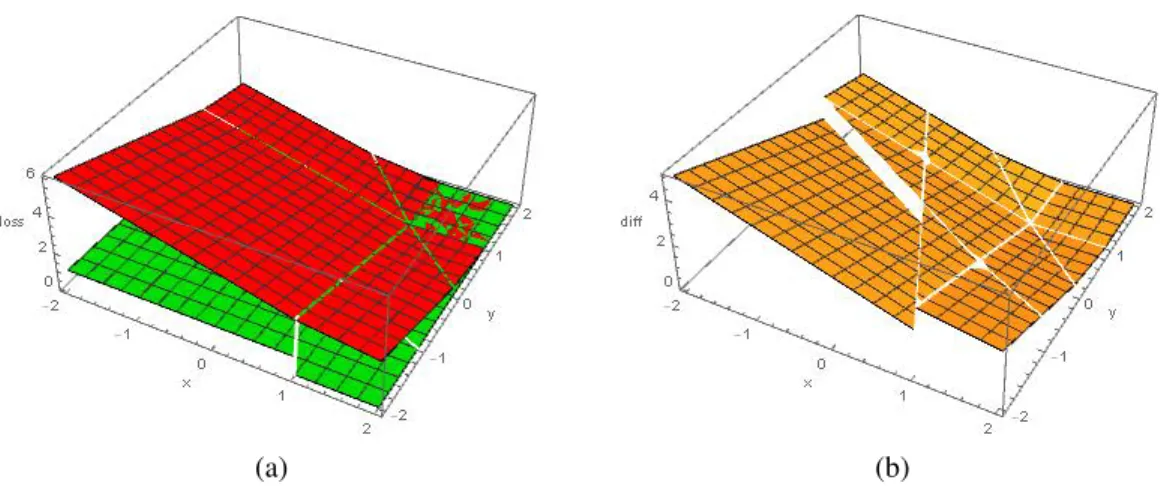
2.1 shows a picture of the effect of the modified loss function when K = 3, γ = 0.5. In this case, g is written as g = (x,y,z) and by symmetry we assume the true class label is 3. We should note that in figure 2.1a, for the interval [1,+∞) ×[1,+∞) there is a mixture of both red and green color. It does not mean our modified loss function cannot bound the indicator function for this interval. It is due to the way that our plotting software Mathematica displays overlapped region. It is clearer in figure 2.1b, in the interval [1,+∞)×[1,+∞) the difference of the two functions remains 0.
(a) (b)
Figure 2.1: Plots of the effect of the modified loss function. In panel (a), the green plane is the indicator functionI(A =d(X)) and the red plane is the proposed modified loss function. Panel (b) is the plot of their difference.
2.3.1.1 Fisher consistency
Before presenting our results about consistency of the optimization problem (2.7), we introduce some assumptions and notations that is specific to this section.
Define conditional reward Rj to be Rj(x) = E[Y|X = x,A = j]. Its positive and negative parts are respectively defined asR+j(x) = E[Y I(Y ≥ 0)|X = x,A = j] andR−
j(x) = E[Y I(Y <
0)|X = x,A = j]. Define the conditional risk function for decision function f asr(f|X = x) =
Ehπ(|AY,|X)VY(f,A)|X = xi
Fisher consistency is an important property in classification literature. Instead of solving the original problem (2.2) we are solving the surrogate problem (2.7). Fisher consistency ensures that the solution to the surrogate problem (2.7) can lead to the solution to the original problem (2.2) given the whole population. A Fisher consistent classifier can achieve the best performance asymptotically. Without any modification, the classifier based on loss function (2.3) is Fisher consistent for 0≤ γ ≤ 0.5 (Zhang et al., 2016). However, if the modification of the loss function is used as in equation (2.6) is used, it becomes more complicated with regard to the consistency. To ensure the consistency, in addition to the three assumptions stated in section 1.2, the following further assumptions need to be imposed
and j respectively. Then R+i(x)>R+t (x)>R+j(x)and R − i(x)>R − t (x)>R − j(x), for∀t,i, j. Also, Rs(x)=R+s(x)+R − s(x)>0, for∀1≤ s≤ K.
Assumption 5 For any treatment s, R+s(x)< P
t,sR+t (x)and R
−
s(x)>
P
t,sR−t (x).
Assumptions 4 and 5 are reasonable in the following sense. First, for any treatment s, R+s(x) and |R−
s(x)|respectively measure the beneficial and adverse effect of treatment s. The larger R+s(x) and |R−s(x)| are, the more beneficial or adverse effects the treatment s have on the patient. Assumption 4 requires that the best treatment should have a large probability of beneficial effect and a small probability of adverse effect while it is contrary for the worst treatment. Second, assumption 5 requires all treatments under consideration are comparable. If, for a treatment s, R+s(x) >
P
t,sR+t(x) or R
−
s(x) <
P
t,sR−t(x), it means the treatment s is a dominantly best or worst treatment which can be identified directly. With assumption 4 and 5, we can obtain the Fisher consistency in the next theorem.
Theorem 2.3.1 If assumptions 4 and 5 are valid, the method of finding optimal treatment rule
using classifier based on the loss function (2.6) is Fisher consistent forγ∈[0,0.5].
If assumptions 4 and 5 do not hold, we can further modify the loss function to make it applicable to all cases. The result is given in theorem 2.3.2.
Theorem 2.3.2 For anyγ ∈ [0,1], if the constrainthf,Wji ≥ − 1
K−1 for any j = 1,· · · ,K is
valid, then the method of finding optimal treatment rule using the classifier based on the loss function (2.6) is still Fisher consistent.
The proofs of theorem 2.3.1 and 2.3.2 are given in the Appendix in this chapter. To make it more explicit, We refer the loss function in theorem 2.3.2 as Vc
Y(f(X),A) wherecdenotes the
constrainthf,Wji ≥ −K1−1 with the loss functionVY(f(X),A). SinceVYc(f(X),A) has an extra constraint compared withVY(f(X),A), it is expected to be less efficient.
2.3.1.2 Computation details
In this section, we derive the dual problem of the optimization (2.7). We focus on both linear and nonlinear case with L2 penalty, and present the results for VY(f(X),A) and VYc(f(X),A) separately.
Loss function 1:VY(f(X),A)
a. Linear case
For linear case, assume that fq(x) = xTβ
q,q= 1,· · · ,K−1, where xis the covariate vector with constant 1 included andβqis the coefficient parameter vector. The penalty term J(f) is defined as J(f) = PK−1
q=1 β
T
qβq. By introducing the slack variablesξi j,i = 1,· · · ,n; j = 1,· · · ,K, the optimization problem can be written as
min βq,ξi j nλ 2 K−1 X q=1 βT qβq+ X i:yi≥0 yi π(Ai,xi)[(1−γ) X j,Ai ξi j+γξi,Ai] − X i:yi<0 yi π(Ai,xi)[(1−γ) X j,Ai ξi j+γξi,Ai] Subject to ξi j ≥0 (i= 1,· · · ,n;j= 1,· · · ,K) ξi,Ai +hf(xi),WAii −(K−1)≥0 (i:yi ≥0) ξi j− hf(xi),Wji −1≥0 (i:yi ≥ 0;j, Ai) ξi,Ai − hf(xi),WAii −(K−1)≥0 (i:yi <0) ξi j+hf(xi),Wji −1≥0 (i:yi < 0;j, Ai)
The Lagrangian functionLcan be defined as
L=nλ 2 K−1 X q=1 βT qβq+ X i:yi≥0 yi π(Ai,xi)[(1−γ) X j,Ai ξi j +γξi,Ai] − X i:yi<0 yi π(Ai,xi)[(1−γ) X j,Ai ξi j+γξi,Ai]− n X i=1 K X j=1 τi jξi j
− X i:yi≥0 αi,Ai[ξi,Ai +hf(xi),WAii −(K−1)]− X i:yi≥0 X j,Ai αi j[ξi j− hf(xi),Wji −1] − X i:yi<0 αi,Ai[ξi,Ai − hf(xi),WAii −(K−1)]− X i:yi<0 X j,Ai αi j[ξi j+hf(xi),Wji −1] = nλ 2 K−1 X q=1 βT qβq+(K−1) n X i=1 αi,Ai + n X i=1 X j,Ai αi j+ X i:yi≥0 K X j=1 [ci j−τi j−αi j]ξi j − X i:yi<0 K X j=1 [ci j +τi j+αi j]ξi j− X i:yi≥0 αi,Aihf(xi),WAii+ X i:yi<0 αi,Aihf(xi),WAii + X i:yi≥0 X j,Ai αi jhf(xi),Wji − X i:yi<0 X j,Ai αi jhf(xi),wji
whereαi j, τi j, i = 1,· · · ,n; j = 1,· · · ,K are Lagrangian multipliers andci j = yi
π(Ai,xi)[(1−
γ)I(j, Ai)+γI(j= Ai)]. By solving ∂β∂L
q =0 and
∂L
∂ξi j = 0, we can obtain that
ci j−τi j−αi j = 0 for i:yi ≥ 0 (2.8) ci j+τi j+αi j = 0 for i:yi < 0 (2.9) βq = 1 nλ h X i:yi≥0 αi,AiWAi,qxi− X i:yi<0 αi,AiWAi,qxi− X i:yi≥0 X j,Ai αi jWjqxi+ X i:yi<0 X j,Ai αi jWjqxi i (2.10)
where Wjq is theq-th component ofWj. Since maximizing Lis equivalent to minimizing
−L, by plugging equation (2.8)∼(2.10) inLwe can obtain the dual problem
min αi j M s.t. 0≤αi j ≤ |ci j| where M= 1 2nλ K−1 X q=1 h X i:yi≥0 αi,AiWAi,qxi− X i:yi<0 αi,AiWAi,qxi − X i:yi≥0 X j,Ai αi jWjqxi+ X i:yi<0 X j,Ai αi jWjqxi iT ×h X i:yi≥0 αi,AiWAi,qxi− X i:yi<0 αi,AiWAi,qxi− X i:yi≥0 X j,Ai αi jWjqxi+ X i:yi<0 X j,Ai αi jWjqxi i
−(K−1) n X i=1 αi,Ai − n X i=1 X j,Ai αi j
Then the optimization problem can be solved by coordinate descent algorithm outlined in Algorithm 1.
Algorithm 1:Estimating fq(x) by coordinate descent algorithm
Result:Estimated decision function fq(x),q=1,· · · ,K−1
Initialization: defineα=(αi j)i=1,···,n;j=1,···,K as ann×K matrix with the (i, j) element equal toαi j. Initializeα(0)as zero matrix andm= 1. N is the maximum number of iterations andtolis the preset tolerance ;
whilem< Ndo
withα(m−1)given, sequentially updateαi j(m−1)toαi j(m). To getα(i jm), first fixα(stm−1),
(s,t),(i, j), solve ∂α∂Mi j = 0 to get solution ˆαi jand the updatedα(
m) i j is determined as α(m) i j = 0 αˆi j ≤0 |ci j| αˆi j ≥ |ci j| ˆ αi j otherwise if |α(m)−α(m−1)|<tolthen
stop the iteration;
else
m= m+1;
end end
Plug ˆαin equation (2.10) to obtain the estimated decision function fq(x), q= 1,· · · ,K−1.
b. Nonlinear case
Define k : X × X → R as a kernel function which is continuous, symmetric and K =
k(xi,xj)
boundary, can be assumed as fq(x)= θq0+P
n
i=1θqik(x,xi). The penalty termJ(f) is defined
as J(f) = PK−1
q=1 θ2q0+
PK−1
q=1 θ
T
qKθq, whereθq = (θq1,· · · , θqn). The optimization problem is
then written as min θq0,θq,ξi j nλ 2 K−1 X q=1 θ2 q0+ nλ 2 K−1 X q=1 θT qKθq+ X i:yi≥0 yi π(Ai,xi)[(1−γ) X j,Ai ξi j +γξi,Ai] − X i:yi<0 yi π(Ai,xi)[(1−γ) X j,Ai ξi j +γξi,Ai] Subject to ξi j ≥ 0 (i= 1,· · · ,n; j=1,· · · ,K) ξi,Ai +hf(xi),WAii −(K−1)≥0 (i:yi ≥0) ξi j− hf(xi),Wji −1≥ 0 (i:yi ≥0; j,Ai) ξi,Ai − hf(xi),WAii −(K−1)≥0 (i:yi <0) ξi j+hf(xi),Wji −1≥ 0 (i:yi <0; j,Ai)
The Lagrangian functionLcan be defined as
L=nλ 2 K−1 X q=1 θ2 q0+ nλ 2 K−1 X q=1 θT qKθq+ X i:yi≥0 yi π(Ai,xi)[(1−γ) X j,Ai ξi j+γξi,Ai] − X i:yi<0 yi π(Ai,xi)[(1−γ) X j,Ai ξi j +γξi,Ai]− n X i=1 K X j=1 τi jξi j − X i:yi≥0 αi,Ai[ξi,Ai +hf(xi),WAii −(K−1)]− X i:yi≥0 X j,Ai αi j[ξi j− hf(xi),Wji −1] − X i:yi<0 αi,Ai[ξi,Ai − hf(xi),WAii −(K−1)]− X i:yi<0 X j,Ai αi j[ξi j+hf(xi),Wji −1] = nλ 2 K−1 X q=1 θ2 q0+ nλ 2 K−1 X q=1 θT qKθq+(K−1) n X i=1 αi,Ai + n X i=1 X j,Ai αi j+ X i:yi≥0 K X j=1 [ci j−τi j−αi j]ξi j − X i:yi<0 K X j=1 [ci j+τi j+αi j]ξi j− X i:yi≥0 αi,Aihf(xi),WAii+ X i:yi<0 αi,Aihf(xi),WAii + X i:yi≥0 X j,Ai αi jhf(xi),Wji − X i:yi<0 X j,Ai αi jhf(xi),wji
whereαi j, τi j,ci j are the same as in linear case. Similarly, by assuming ∂ξ∂L i j = 0, ∂L ∂θq0 = 0 and ∂θ∂L q =0, we obtain ci j−τi j−αi j = 0 for i:yi ≥0 (2.11) ci j+τi j+αi j = 0 for i:yi <0 (2.12) θq0 = 1 nλ h X i:yi≥0 αi,AiWAi,q− X i:yi<0 αi,AiWAi,q− X i:yi≥0 X j,Ai αi jWjq+ X i:yi<0 X j,Ai αi jWjq i (2.13) θq= 1 nλK −1h X i:yi≥0 αi,AiWAi,qKi− X i:yi<0 αi,AiWAi,qKi− X i:yi≥0 X j,Ai αi jWjqKi+ X i:yi<0 X j,Ai αi jWjqKi i (2.14)
whereKi is theith column of the gram matrixKandWjq is the same as in linear case. By plugging equation (2.11)∼(2.14) inL, we obtain the dual problem
min αi j M s.t. 0≤αi j ≤ |ci j| where M = 1 2nλ K−1 X q=1 h X i:yi≥0 αi,AiWAi,qKi− X i:yi<0 αi,AiWAi,qKi− X i:yi≥0 X j,Ai αi jWjqKi + X i:yi<0 X j,Ai αi jWjqKi iT K−1 ×h X i:yi≥0 αi,AiWAi,qKi− X i:yi<0 αi,AiWAi,qKi− X i:yi≥0 X j,Ai αi jWjqKi+ X i:yi<0 X j,Ai αi jWjqKi i + 1 2nλ K−1 X q=1 h X i:yi≥0 αi,AiWAi,q− X i:yi<0 αi,AiWAi,q− X i:yi≥0 X j,Ai αi jWjq+ X i:yi<0 X j,Ai αi jWjq i2 −(K−1) n X i=1 αi,Ai − n X i=1 X j,Ai αi j
Loss function 2:VYc(f(X),A)
Unlike SVM whose solution only depends on support vectors, the classifier based onVYc(f(X),A) uses all training data to estimate the decision function. The conditionhf,Wji ≥ −K1−1 can typ-ically be approximated by modifying the loss function so that huge loss will be added when
hf,Wji<−K1−1 (Park and Liu, 2009). Thus we define a new loss function
lu(f(X),A)= VY(f(X),A) hf(X),Ai ≥ −K1−1 u(−K1−1 − hf(X),Ai) hf(X),Ai<−K1−1 (2.15)
where u ≥ 0 and VY(f(X),A) is defined in equation (2.6). When u → +∞, lu(f(X),A) →
VYc(f(X),A). So the optimization problem can be written as
minnλ 2 J(f)+ X i:yi≥0 yi π(Ai,xi) (1−γ)X j,Ai ξi j+γξi,Ai − X i:yi<0 yi π(Ai,xi) (1−γ)X j,Ai ξi j+γξi,Ai Subject to ξi j ≥0 (i= 1,· · · ,n; j=1,· · · ,K) ξi,Ai +hf(xi),WAii −(K−1)≥0 (i:yi ≥0) ξi j− hf(xi),Wji −1≥ 0 (i:yi ≥ 0;j, Ai) ξi,Ai − hf(xi),WAii −(K−1)≥0 (i:yi <0) ξi j+hf(xi),Wji −1≥ 0 (i:yi < 0;j, Ai) ξi j+u( 1 K−1 +hf(xi,Wji)≥0 (i=1,· · · ,n; j=1,· · · ,K) The corresponding Lagrangian function Lcan be defined as
L= nλ 2 J(f)+(K−1) n X i=1 αi,Ai + n X i=1 X j,Ai αi j+ X i:yi≥0 K X j=1 [ci j−τi j−αi j−vi j]ξi j − X i:yi<0 K X j=1 [ci j+τi j+αi j+vi j]ξi j − X i:yi≥0 αi,Aihf(xi),WAii+ X i:yi<0 αi,Aihf(xi),WAii
+ X i:yi≥0 X j,Ai αi jhf(xi),Wji − X i:yi<0 X j,Ai αi jhf(xi),wji − n X i=1 K X j=1 vi juhf(xi),Wji − n X i=1 K X j=1 vi j u K−1
whereci j,αi jandτi jare defined the same as before andvi jis the Lagrangian multiplier for the inequality constraintξi j +u(K1−1 +hf(xi,Wji)≥ 0. For linear decision rule,J(f)= P
K−1
q=1 βTqβq. For nonlinear decision rule, J(f) = PK−1
q=1 θ2q0+
PK−1
q=1 θ
T
qKθq. After some similar mathematical operations as in the case ofVY(f(X),A), for both linear and nonlinear cases we have
ci j −τi j −αi j−vi j = 0 for i:yi ≥ 0 ci j +τi j +αi j+vi j = 0 for i:yi < 0 (2.16)
For linear decision rule,βq,q= 1,· · · ,K−1 are functions ofαi j,vi j,i=1,· · · ,n; j=1,· · · ,K as βq = 1 nλ h X i:yi≥0 αi,AiWAi,qxi− X i:yi<0 αi,AiWAi,qxi− X i:yi≥0 X j,Ai αi jWjqxi + X i:yi<0 X j,Ai αi jWjqxi+ n X i=1 K X j=1 vi juWjqxii (2.17)
For nonlinear decision rule,θq0 andθq,q= 1,· · · ,K−1 can be obtained by
θq0 = 1 nλ h X i:yi≥0 αi,AiWAi,q− X i:yi<0 αi,AiWAi,q− X i:yi≥0 X j,Ai αi jWjq + X i:yi<0 X j,Ai αi jWjq+ n X i=1 K X j=1 vi juWjq i (2.18) θq= 1 nλK −1h X i:yi≥0 αi,AiWAi,qKi− X i:yi<0 αi,AiWAi,qKi− X i:yi≥0 X j,Ai αi jWjqKi + X i:yi<0 X j,Ai αi jWjqKi+ n X i=1 K X j=1 vi juWjqKi i (2.19)
So the dual problem for linear case is
min
αi j M
s.t. 0≤αi j+vi j ≤ |ci j| where M = 1 2nλ K−1 X q=1 h X i:yi≥0 αi,AiWAi,qxi− X i:yi<0 αi,AiWAi,qxi− X i:yi≥0 X j,Ai αi jWjqxi+ X i:yi<0 X j,Ai αi jWjqxi + n X i=1 K X j=1 vi juWjqxi iT ×h X i:yi≥0 αi,AiWAi,qxi− X i:yi<0 αi,AiWAi,qxi− X i:yi≥0 X j,Ai αi jWjqxi + X i:yi<0 X j,Ai αi jWjqxi+ n X i=1 K X j=1 vi juWjqxii−(K−1) n X i=1 αi,Ai − n X i=1 X j,Ai αi j+ n X i=1 K X j=1 vi j u K−1
The dual problem for nonlinear case is
min αi j,vi j M s.t. 0≤αi j+vi j ≤ |ci j| where M = 1 2nλ K−1 X q=1 h X i:yi≥0 αi,AiWAi,qKi− X i:yi<0 αi,AiWAi,qKi− X i:yi≥0 X j,Ai αi jWjqKi+ X i:yi<0 X j,Ai αi jWjqKi + n X i=1 K X j=1 vi juWjqKi iT K−1×h X i:yi≥0 αi,AiWAi,qKi − X i:yi<0 αi,AiWAi,qKi− X i:yi≥0 X j,Ai αi jWjqKi + X i:yi<0 X j,Ai αi jWjqKi+ n X i=1 K X j=1 vi juWjqKi i + 1 2nλ K−1 X q=1 h X i:yi≥0 αi,AiWAi,q− X i:yi<0 αi,AiWAi,q − X i:yi≥0 X j,Ai αi jWjq+ X i:yi<0 X j,Ai αi jWjq+ n X i=1 K X j=1 vi juWjq i2 −(K−1) n X i=1 αi,Ai − n X i=1 X j,Ai αi j + n X i=1 K X j=1 vi j u K−1
2.3.2
Multi-stage
In this section we considerT > 1. Q-learning uses backwards induction forT > 1. The prin-ciple is that the best treatment at the last stage is first estimated and then we move backwards to the previous stages. A brief example of two-stage case is given in section 1.4.1. For our proposed method, we use a similar technique as inQ-learning with a difference in the pseudo-outcome. Since Q-learning models the conditional mean outcome at each staget = 1,· · · ,T, the pseudo-outcome is generated via the maximizedQ-function in the next stage where theQ function is typically approximated by regression models. In our proposed method, we directly estimate the best treatment based on the pseudo-outcome obtained via the potential outcome as if the patients receive the estimated best treatment in all future stages using the doubly-robust estimator (Zhang et al., 2013).
We define a Q-function at staget, Qt, as the reward obtained in future stages if the patient is assigned the estimated optimal treatment from stage t to the end stage T. Based on the definition, we have QT+1 = 0 and for t = 1,· · · ,T, if a patient actually follows the estimated
best treatment from stage t to the end, Qt = PT
s=tYs, otherwise it will be approximated by
the doubly-robust estimator which will be described later. The pseudo-outcome at stage t = 1,· · · ,T,Ytpse, is then defined asY
pse
t =Yt +Qt+1.
We can recast the estimation of potential outcome provided that patients follow the es-timated best treatment from stage t to the end as a monotone coarsening problem, and it is shown that coarsening is at random (Zhang et al., 2013). For estimatingQt, we start from stage tand all history information prior to stagetis viewed as the new baseline information. Define Nts = I(At = dt,· · · ,As = ds),t < s as an indicator function for whether or not the patient receives the recommended treatment from stagetto s. Then we define the coarsening discrete hazard λts( ¯Xs) = Pr(As , ds( ¯Xs,As¯ −1)|Xs¯ ,Nt,s−1 = 1). It is the probability that the treatment
received by patients ceases to be consistent with the dynamic treatment regimes d at stage s given that it is consistent from stagetto stage s−1. The probability of the observed treatment being consistent withdt at least up to stagescan be expressed as Mts( ¯Xs)=Qs
Then the doubly-robust estimator ofQt(Zhang et al., 2013) is constructed as Qt = NtT PT s=tYs MtT( ¯XT) + T X s=t Nt,s−1(I[As, ds( ¯Xs)]−λts( ¯Xs)) Mts( ¯Xs) Lts( ¯Xs) (2.20)
whereLts( ¯Xs) can be arbitrary function of ¯Xsand the optimal choice with the smallest asymp-totic variance isE[Qt|Xs¯ ,Nt,s−1= 1] (Zhang et al., 2013).
From equation (2.20) we need to estimateλts( ¯Xs) and Lts( ¯Xs). For the estimation ofλts( ¯Xs) we only need to specify the model for propensity score πs( ¯xs,as¯ −1,as) = Pr(As = as|Xs¯ =
xs,As¯ −1 = as¯ −1). For randomized trial, πs( ¯xs,as¯ −1,as) is determined. For observational study
πs( ¯xs,as¯ −1,as) needs to be modeled. A common choice to obtain the propensity score is the
lo-gistic regression or multinomial regression. LetLts( ¯Xs)=1−π( ¯Xs,at−1,dts−1( ¯Xs−1),ds( ¯Xs)) and
takeLts( ¯Xs)= E[Qt|Xs¯ ,Nt,s−1 =1]. We can define iteratively thatµtT( ¯xt,at)¯ = E[PTp=tYp|XT¯ =
¯
xT,AT¯ = aT¯ ] and ftT( ¯xT,aT¯ −1) = µtT( ¯xT,aT¯ −1,dT). For s = T −1,· · · ,t, define µts( ¯xs,as)¯ =
E[ft,s+1( ¯xs,Xs+1,as¯ |Xs¯ = xs¯ ,As¯ = as] and¯ fts( ¯xs,as¯ −1) = µts( ¯xs,as¯ −1,ds). It is shown that
Lts( ¯Xs)= µts( ¯xs,ds
t) (Zhang et al., 2013).
2.4
Numerical investigation
In this section, we describe both the simulation studies and real data application of the proposed method.
2.4.1
Simulation study
To assess the performance of the proposed methods, simulation studies were carried out for a variety of scenarios. We consider both linear and nonlinear decision rule with single stage and multi-stage. For linear decision rule, we restrict f to be a linear function ofxand for nonlinear decision rule we use Gaussian kernel. We also evaluate the influence of reduced main effect, reduced interaction effect as well as increased number of treatments.
For each simulation setting, we first generate a tuning set with a sample size of 500 for training the tuning parameter which is λin linear case and λ, τ in nonlinear case. We use a grid search to find the best tuning parameter. λvaries in [0.1,100] and τin Gaussian kernel
k(x,y) = exp{−||x−y||2
2/(2τ
2)}varies in [0.1,2]. For the parameteruin Vc
Y(f(X),A), we just
useu = 1000 because whenubecomes larger than 1000 the result will not change much. For each of our settings, we repeat the simulation 500 times. For each simulation run, we gener-ate a data set with a sample size of 1500. We randomly choose 500 of them as training data and the remaining is used as testing data. For single stage, we use misclassification error rate and the empirical value function to assess the performance of the model. For multi-stage, we only use empirical value function to assess the model. The misclassification error rate in the single stage setting is defined asPn[I(Aopt = d(X))] and the empirical value function is defined asPn[QT t=1 I(At=dt(Ht)) πt(At|Ht)Y ]/Pn[ QT t=1 I(At=dt(Ht))
πt(At|Ht) ] wherePn is the empirical average operator. The mis-classification error rate measures the possibility that the estimated dynamic treatment regime cannot detect the true optimal treatment. The empirical value function measures the outcome patients can obtain if they follow the estimated dynamic treatment regime. A smaller misclas-sification error rate or a larger empirical value function provide evidence that the estimated dynamic treatment regime is preferred.
We consider 9 scenarios (Liu and Yuan, 2011; Zhang et al., 2016):
1. A three-treatment case. The optimal treatment Aopt satisfies Pr(Aopt = 1) = Pr(Aopt = 2) = Pr(Aopt = 3) = 1/3. The covariate vector satisfiesX|Aopt = j ∼ N(µ
j, σ2I) where µ1 = (1,0,0)T, µ2 = (−0.5, √ 3/2,0)T, µ 3 = (−0.5,− √
3/2,0)T, σ2 is chosen such that
the Bayes classification error is 5% andI is the identity matrix. The actual treatment is generated from multinomial distribution with
Pr(Aobs =1|X)= 1
1+exp(−2+X1+2X2−X3)+exp(−1−2X1+2X2)
Pr(Aobs =2|X)= exp(−2+X1+2X2−X3)
Pr(Aobs =3|X)= exp(−1−2X1+2X2)
1+exp(−2+X1+2X2−X3)+exp(−1−2X1+2X2)
The outcomeRfollows N(xTβ+10I(Aobs =Aopt),1) whereβ=(0,1,1)T.
2. All the settings are the same as scenario 1 except thatβ=0.1×(0,1,1)T.
3. All the settings are the same as scenario 1 except that R follows N(xTβ + 2I(Aobs =
Aopt),1)
4. A four-treatment case. The optimal treatment Aopt satisfies Pr(Aopt = 1) = Pr(Aopt = 2) = Pr(Aopt = 3) = Pr(Aopt = 4) = 1/4. The covariate vector satisfies X|Aopt = j ∼
N(µj, σ2I) whereµj = (Wj,0,0)T, Wj is defined in section 2.2 when K = 4 andσ2 is
chosen such that the Bayes classification error is 5% and I is the identity matrix. The actual treatment is generated from multinomial distribution with
Pr(Aobs =1|X)= 1
S
Pr(Aobs =2|X)= exp(−2+X1+2X2−X3)
S
Pr(Aobs =3|X)= exp(−1−2X1+2X2)
S
Pr(Aobs =4|X)= exp(−2X1+2X2−2X4−X5)
S
whereS =1+exp(−2+X1+2X2−X3)+exp(−1−2X1+2X2)+exp(−2X1+2X2−2X4−X5)
The outcomeRfollowsN(xTβ+10I(Aobs = Aopt),1) whereβ= (0,1,−1,1,−1)T. 5. All the settings are the same as scenario 1 except that the covariate vector satisfies
X|Aopt = j ∼ 0.5N(µja, σ2I)+ 0.5N(µjb, σ2I) where µja = (cos(jπ/3),sin(jπ/3),0)T,
µjb = (cos(jπ/3+π),sin(jπ/3+π),0)T,σ2is chosen such that the Bayes classification error is 5% andIis the identity matrix.
7. All the settings are the same as scenario 5 except that R follows N(xTβ + 2I(Aobs =
Aopt),1)
8. All the settings are the same as scenario 4 except that the covariate vector satisfies
X|Aopt = j ∼ 0.5N(µ
ja, σ2I)+ 0.5N(µjb, σ2I) whereµja = (cos(jπ/4),sin(jπ/4),0T3)T,
µjb = (cos(jπ/4+ π),sin(jπ/4+ π),0T3)T, σ2 is chosen such that the Bayes classifica-tion error is 5% and I is the identity matrix. The actual treatment is generated from multinomial distribution with
Pr(Aobs =1|X)= 1
S
Pr(Aobs =2|X)= exp(−2+X1+2X2−X3−2X4)
S
Pr(Aobs =3|X)= exp(−1−2X1+2X2−2X5)
S Pr(Aobs =4|X)= exp(X1−X3−X4)
S
whereS =1+exp(−2+X1+2X2−X3−2X4)+exp(−1−2X1+2X2−2X5)+exp(X1−X3−X4)
9. A two-stage case. The optimal treatment at stage t, Aoptt ,t = 1,2 satisfies Pr(Aoptt = 1) = Pr(Aoptt = 2) = Pr(A
opt
t = 3) = 1/3. The covariate vector at stage t satisfies
Xt|Aoptt = j ∼ 0.5N(µja, σ2I)+0.5N(µjb, σ2I) where µja = (cos(jπ/3),sin(jπ/3),0T3)T,
µjb = (cos(jπ/3+π),sin(jπ/3+π),0T3)T,σ2is chosen such that the Bayes classification error is 5% andIis the identity matrix. The actual treatment at stage 1 is generated from multinomial distribution with
Pr(Aobs1 =1|X1)= 1 S Pr(Aobs1 =2|X1)= exp(−1−X11+2X12−X13−X14−X15) S Pr(Aobs1 =3|X1)= exp(−1−2X11+2X12−2X13+2X14) S
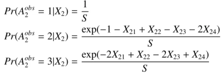
The actual treatment at stage 2 is generated from multinomial distribution with Pr(Aobs2 =1|X2)= 1 S Pr(Aobs2 =2|X2)= exp(−1−X21+X22−X23−2X24) S Pr(Aobs2 =3|X2)= exp(−2X21+X22−2X23+X24) S
whereS = 1+exp(−1−X21+X22−X23−2X24)+exp(−2X21+X22−2X23+X24). The
outcomeR1 follows N(u1,1) where u1 = 10I(A
opt 1 = A obs 1 )+ X12+ X13− X 2 14+ X11X15.
The outcomeR2followsN(u2,1) whereu2 =5I(A
opt 2 = A obs 2 )+(X 2 22+X24) 2X 21+X23X25.
Scenarios 1 ∼ 4 have linear decision rule and scenarios 5 ∼ 8 have nonlinear decision rule. Scenarios 2 and 6 involve reduced main effect while scenarios 3 and 7 investigate the impact of the reduced interaction effect. Scenarios 4 and 8 consider a four-treatment case so that the effect of the number of treatment options can be observed. Finally, scenario 9 involves two stages as well as a more complex nonlinear main effect.
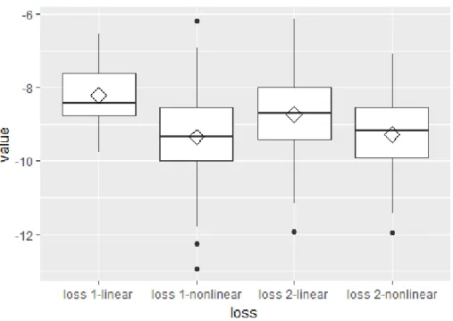
Figure 2.2 shows the simulation results for scenarios 1 and 5 using different values ofγ. Loss 1 refers to the unconstrained loss functionVY(f(X),A), while loss 2 refers toVc
Y(f(X),A). It is shown in the figure that forVYc(f(X),A) the simulation results do not vary much for diff er-entγ, compared withVY(f(X),A). For linear case,VY(f(X),A) outperformsVYc(f(X),A) while for nonlinear caseVYc(f(X),A) performs better. γ = 0.5 gives relatively stable results. γ = 0.5 may not perform the best in a single case but it always gives results close to the best one. Con-sidering this observation and the fact thatVY(f(X),A) is Fisher consistent in [0,0.5], in other scenarios, we useγ =0.5.
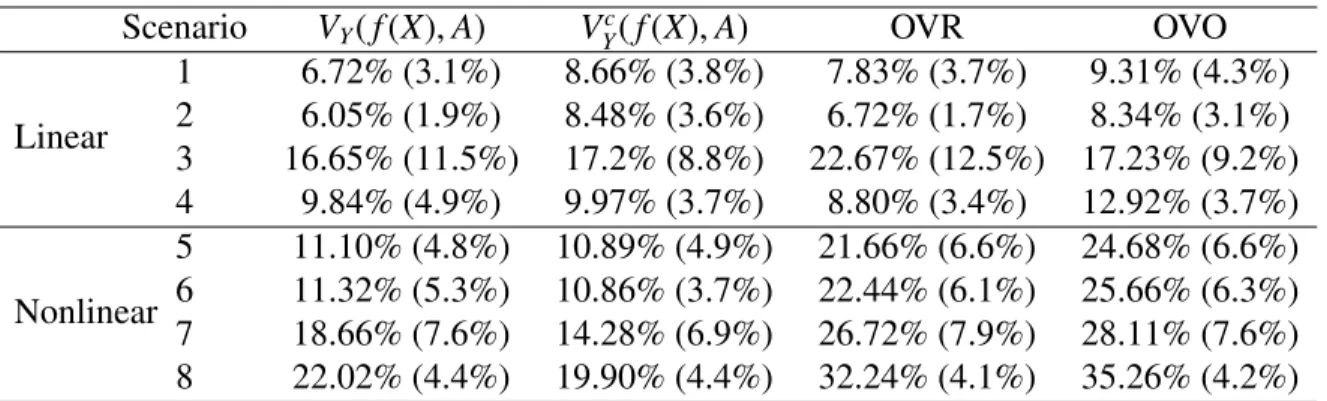
Table 2.1 shows the misclassification error rates obtained by validation data of size 1000, where OVR and OVO columns are results from One-Versus-Rest and One-Versus-One meth-ods. The One-Versus-Rest approach constructs K classifiers each comparing one of the K classes to the remaining K − 1 classes and producing a real-valued confidence score for its prediction. A new observation is assigned to the class for which the corresponding classifier
(a) (b)
(c) (d)
Figure 2.2: Simulation results for scenarios 1 and 5 for different γ. Loss 1 and 2 refer to
VY(f(X),A) andVYc(f(X),A) respectively. Figure 2.2a and figure 2.2b show the
misclassifica-tion error rates and empirical value for linear decision boundary. Figure 2.2c and figure 2.2d give the same result for nonlinear decision boundary
produces the highest confidence score. The One-Versus-One approach constructs K(K2−1) clas-sifiers each comparing a pair of classes. A new observation is assigned to the class to which it is most frequently assigned in these K(K2−1) pairwise classifications. From table 2.1, in terms of misclassification error rates, VY(f(X),A) performs better than VYc(f(X),A) in the first two scenarios and they have comparable performance for scenarios 3 ∼ 6. However, for scenar-ios 7 and 8, misclassification error rates obtained fromVYc(f(X),A) are apparently lower than those obtained fromVY(f(X),A). Also, estimates obtained fromVYc(f(X),A) have comparable or smaller standard deviations than those fromVY(f(X),A) in all scenarios except scenario 2. These observations show that Vc
Y(f(X),A) is better at dealing with complex situation and is
more stable as expected given that the Fisher consistency of classifier based on Vc
Y(f(X),A) does not require any assumptio