Smoothing in Probability Estimation Trees

(1)

http://researchcommons.waikato.ac.nz/

Research Commons at the University of Waikato

Copyright Statement:

The digital copy of this thesis is protected by the Copyright Act 1994 (New Zealand). The thesis may be consulted by you, provided you comply with the provisions of the Act and the following conditions of use:

 Any use you make of these documents or images must be for research or private study purposes only, and you may not make them available to any other person.

 Authors control the copyright of their thesis. You will recognise the author’s right to be identified as the author of the thesis, and due acknowledgement will be made to the author where appropriate.

 You will obtain the author’s permission before publishing any material from the thesis.

(2)

Department of Computer Science

Hamilton, NewZealand

Smoothing in Probability

Estimation Trees

Zhimeng Han

This thesis is submitted in partial fulfilment of the requirements for the degree of Master of Science at The University of Waikato.

March 2011 c

(3)

(4)

Abstract

Classification learning is a type of supervised machine learning technique that uses a classification model (e.g. decision tree) to predict unknown class labels for previously unseen instances. In many applications it canbe very useful to additionally obtain class probabilities for the different class labels. Decision trees that yield these probabilities are also called probability estimation trees(PETs). Smoothing is a technique used to improve the probability estimates. There are several existing smoothing methods, such as the Laplace correction (Provost & Domingos, 2003), M-Estimate smoothing (Dzeroski, Cestnik & Petrovski, 1993) and M-Branch smoothing (Ferri, Flach & Hern´andez-Orallo, 2003). Smoothing does not just apply to PETs. In the field of text compression, PPM (Cleary & Witten, 1984) in particular, smoothing methods play a important role. This thesis migrates smoothing methods from text compression to PETs. The newly migrated methods in PETs are compared with the best of the existing smoothing methods considered in this thesis under different experiment setups. Unpruned, pruned and bagged tree are considered in the experiments. The main finding is that the PPM-based methods yield the best probability estimates when used with bagged trees, but not when used with individual (pruned or unpruned) trees.

(5)

(6)

Acknowledgments

I would like to thank my supervisor Assoc. Prof. Eibe Frank for the guidance throughout not just the thesis, but also with code implemented in Weka. He provided extensive help and materials for the problems I encountered during the thesis write up and the development. He guided me with lots of patience and understanding.

I would also like to thank Sun Quan, who is a member of the machine learning group at the University of Waikato. He gave me lots of help with the UCSD machine learning competition.

(7)

(8)

Contents

Abstract i

Acknowledgments iii

1 Introduction 1

1.1 Basic machine learning concepts . . . 2

1.2 Probability estimation trees . . . 2

1.2.1 Smoothing . . . 3

1.2.2 Cost sensitive classification . . . 5

1.3 Motivation and Objectives . . . 6

1.4 Thesis Structure . . . 6

2 Background and Related work 9 2.1 Learning Tree Classifiers . . . 9

2.1.1 Pruning . . . 10

2.1.2 Adjusting probability estimates . . . 11

2.2 Bagging trees . . . 12

2.3 Text compression and PPM . . . 13

2.3.1 PPM . . . 13

2.4 Datasets . . . 14

2.5 Evaluation methods . . . 16

2.5.1 Root mean squared error . . . 17

2.5.2 Area under ROC curve . . . 17

2.5.3 Entropy gain . . . 18

2.6 Summary . . . 18

3 Smoothing methods 21 3.1 Existing smoothing methods in probability estimation trees . . . 21

3.1.1 Laplace Correction and M-Estimate . . . 21

3.1.2 M-Branch Smoothing . . . 22

(9)

3.2.1 PPMA . . . 23 3.2.2 PPMB . . . 24 3.2.3 PPMC . . . 25 3.2.4 PPMD . . . 26 3.2.5 PPMP . . . 27 3.3 Smoothing effects . . . 28

3.4 Implementing the smoothing methods . . . 28

3.4.1 M-Branch Smoothing . . . 29

3.4.2 PPM Methods . . . 30

3.5 Summary . . . 31

4 Experiments 35 4.1 Methodology and Experiment Setups . . . 35

4.2 Smoothing effect of M-Estimate smoothing and the Laplace correction . . . 36

4.3 M-Estimate versus M-Branch . . . 39

4.4 M-Branch smoothing versus PPM smoothing methods . . . 42

4.5 Effect of Bagging Trees . . . 45

4.6 Bagging with simple smoothing methods . . . 46

4.7 M-Branch smoothing with Bagging . . . 48

4.8 PPM with Bagging . . . 51 vi

(10)

4.9 Smoothing pruned trees . . . 54

4.10 Pruning with simple smoothing methods . . . 55

4.10.3 Entropy gain . . . 57

4.11 M-Branch smoothing on pruned trees . . . 58

4.11.3 Entropy gain . . . 60

4.12 PPM with pruning . . . 61

4.12.3 Entropy gain . . . 63

4.13 Case study: UCSD machine learning competition . . . 64

4.13.1 Dataset and Experiment setup . . . 64

4.13.2 Simple smoothing methods . . . 65

4.13.3 M-Branch smoothing . . . 66

4.13.4 PPM smoothing methods . . . 66

5 Conclusions 69 5.1 Summary and conclusion . . . 69

5.2 Future work . . . 71 A More experimental results for bagged trees and pruned trees vs

(11)

(12)

List of Figures

1.1 A PET built with Iris data . . . 3

1.2 ROC curve with and without smoothing . . . 5

2.1 Pseudo code for constructing a PET . . . 10

2.2 Pseudo code for making a prediction using a PET . . . 10

2.3 Unpruned PET for iris data . . . 11

2.4 Pseudo code for bagging . . . 13

2.5 Pseudo code for prediction with bagging . . . 13

2.6 Example ROC curves . . . 18

3.1 Pseudo code for Laplace correction in REPTree . . . 28

3.2 Pseudo code for M-Estimate in REPTree . . . 29

3.3 Pseudo code for height calculation in REPTree . . . 29

3.4 Pseudo code for M-Branch smoothing in REPTree . . . 30

3.5 Pseudo code for PPM in REPTree . . . 30

3.6 Pseudo code for getProduct in REPTree . . . 31

3.7 Pseudo code for getEscProb method in REPTree . . . 32

4.1 ROC curves of simple smoothing methods . . . 66

4.2 ROC curves of M-Estimate vs M-Branch smoothing . . . 67

(13)

(14)

List of Tables

1.1 The iris data . . . 3

1.2 The iris data . . . 4

2.1 Datasets used in experiments . . . 14

3.1 M-Branch smoothing effects along a path of prediction . . . 23

3.2 PPMA smoothing effects along a path of prediction . . . 24

3.3 PPMB smoothing effects along a path of prediction . . . 25

3.4 PPMC smoothing effects along a path of prediction . . . 26

3.5 PPMD smoothing effects along a path of prediction . . . 27

3.6 Smoothing effects compared . . . 28

4.1 Area under ROC curve . . . 37

4.2 Root mean squared error . . . 38

4.3 Entropy gain . . . 39

4.4 Area under ROC curve (M-Estimate vs M-Branch) . . . 40

4.5 Root mean squared error (M-Estimate vs M-Branch) . . . 41

4.6 Entropy gain (M-Estimate vs M-Branch) . . . 41

4.7 Area under ROC curve (M-Branch vs PPM methods) . . . 43

4.8 Root mean squared error (M-Branch vs PPM methods) . . . 44

4.9 Entropy gain (M-Branch vs PPM methods) . . . 45

4.10 Area under ROC curve . . . 46

4.11 Area under ROC curve with Bagging . . . 47

4.12 Root mean squared error with bagging . . . 48

4.13 Entropy gain with bagging . . . 49

4.14 Area under ROC curve with bagging (Laplace correction vs M-Branch) . . 50

4.15 Root mean squared error with bagging (Laplace correction vs M-Branch) . 51 4.16 Entropy gain with bagging(Laplace correction vs M-Branch) . . . 52

4.17 Area under ROC curve (Laplace correction vs PPM methods . . . 53

4.18 Root mean squared error (Laplace correction vs PPM methods) . . . 54

(15)

4.20 Area under ROC curve (No smoothing vs No smoothing pruned) . . . 56

4.21 Area under ROC curve with pruning . . . 57

4.22 Root mean squared error with pruning . . . 58

4.23 Entropy gain with pruning . . . 59

4.24 Area under AUC curve with pruning (M-Estimate vs M-Branch) . . . 60

4.25 Root mean squared error with pruning (M-Estimate vs M-Branch) . . . 61

4.26 Entropy gain with pruning (M-Estimate vs M-Branch) . . . 62

4.27 Area under ROC curve with pruning(M-Branch vs PPM methods . . . 63

4.28 Root mean squared error with pruning (M-Branch vs PPM methods) . . . . 64

4.29 Entropy gain with pruning (M-Branch vs PPM methods) . . . 65

A.1 Root mean squared error with bagging . . . 73

A.2 Entropy gain with bagging . . . 74

A.3 Root mean squared error with pruning . . . 74

A.4 Entropy gain with pruning . . . 75

(16)

Chapter 1

Introduction

Consider the following definition of machine learning, as given by Arthur Samuel (Samuel, 1959):

Machine learning is the field of study that gives computers the ability to learn without being explicitly programmed.

In machine learning, there are many ways to achieve the goal, such as regression, classification and clustering. This thesis investigates a learning technique called prob-ability estimation tree learning. It evaluates how well smoothing methods used in text compression work in probability estimation trees. Can smoothing methods from text compression be used to improve the accuracy of the probability estimates provided by probability estimation trees?

Probability estimation is important in cost-sensitive classification. In practical classification tasks, there are errors in predictions made by the learner. Some errors have a higher cost than others, and it is best to minimize the cost of errors when making predictions. Information on miss-classification costs can be used to build cost-sensitive models or make cost sensitive predictions by minimizing the expected cost (Witten & Frank, 2005). Class probabilities can be used to perform cost-sensitive predictions, but accurate probability estimates are needed to yield good performance.

The remainder of this chapter is structured as follows. Section 1.1 outlines the ba-sic concepts. Section 1.2 discusses the ideas necessary for understanding probability estimation trees. Section 1.2.1 covers the basics about smoothing. Section 1.3 introduces the motivation and objectives of this thesis. Section 1.4 lists the structure of the rest of this thesis.

(17)

1.1

Basic machine learning concepts

As discussed above, machine learning is a set of techniques that discovers and extracts patterns from data. The process will involve the input data, and the output. The input involves datasets, attributes and instances. Tables 1.1 and 1.2 each show a small part of a dataset. The rows of the table are instances, and each row represents a single instance in the dataset. The columns are attributes: sepal length, sepal width, petal length, petal width and flower type are the attributes in the iris dataset.

The learning process, is a potentially complex process that can involves various techniques such as classification, regression, clustering and association. Classification learning takes a dataset, which has instances with class labels, to build a model based on this data. Then it applies the model to data that does not have any class label to predict the class value. In contrast, clustering divides the data into several natural groups instead of labeling each instance with a class value based on labeled training data. Regression is similar to classification, but it uses numeric values as class labels. Association learning is the technique that finds all kinds of relationships between instances, and does not just predicting the class values.

1.2

Probability estimation trees

A probability estimation tree (PET) is a model used in classification learning. It is built using a dataset with class values, and used to predict class probabilities for previously unseen data without class values.

PETs are usually constructed using a top-down fashion. One of the attributes will be selected to define the split at the root node. The way to choose which attribute to split on is to measure the purity of the child nodes after the split. The most common measure-ment of impurity is called information (Quinlan, 1986) or entropy (Witten & Frank, 2005).

Figure 1.1 shows a PET induced for the iris data. As mentioned above, table 1.2 shows an excerpt of this data. The last column is the class attribute. The 5 attributes in total: sepal length, sepal width, petal length, petal width and class values. The tree predicts probabilities for the class values given the other attributes. In this case only two of the attributes are used in the tree.

(18)

Sepal length Sepal width Petal length Petal width Flower type

6.0 2.9 4.5 1.5 Unknown

Table 1.1: The iris data

1: petallength 2 : Iris-setosa (1,0,0) < 2.5 3: petalwidth >= 2.5 4 : Iris-versicolor (0,0.907,0.093) < 1.75 5 : Iris-virginica (0,0.022,0.978) >= 1.75

Figure 1.1: A PET built with Iris data

The tree can be used to read off probability estimates for new test cases. For ex-ample assume we are predicting an iris flower with attribute values shown in Table 1.1: Prediction starts at the root of tree, where the splitting attribute is petal length. The petal length of the iris is greater than 2.5, so we go to the right branch. The second split attribute is petal width, and petal width of the iris is less than 1.75, so we follow the left branch. Then we do not have any further splits, so we can conclude this iris is of type versicolor, and the predicted probability is 0.907. The estimated probabilities for the other classes are: Iris-setosa 0, Iris-virginica 0.093.

1.2.1 Smoothing

Smoothing is a technique widely used in the field of machine learning to compensate for data sparseness. Lack of data can lead to highly variable estimates. Smoothing provides a way to make estimates more robust. Smoothing is used in other fields too, such as text compression. The text compression method PPM (Prediction by Partial Matching) and its variants (PPMD, PPMP and etc.) are widely used in everyday application. In (Bell, Cleary & Witten, 1990), three smoothing methods that are generally used in PPM are introduced. This thesis empirically investigates the performance of these smoothing methods when used in PETs. Without smoothing, probability estimates at the leaf

(19)

Sepal length Sepal width Petal length Petal width Flower type 1 5.1 3.5 1.4 0.2 Iris-setosa 2 4.9 3.0 1.4 0.2 Iris-setosa 3 4.7 3.2 1.3 0.2 Iris-setosa 4 4.6 3.1 1.5 0.2 Iris-setosa 5 5.0 3.6 1.4 0.2 Iris-setosa . . . 51 7.0 3.2 4.7 1.4 Iris-versicolor 52 6.4 3.2 4.5 1.5 Iris-versicolor 53 6.9 3.1 4.9 1.5 Iris-versicolor 54 5.5 2.3 4.0 1.3 Iris-versicolor 55 6.5 2.8 4.6 1.5 Iris-versicolor . . . 101 6.3 3.3 6.0 2.5 Iris-virginica 102 5.8 2.7 5.1 1.9 Iris-virginica 103 7.1 3.0 5.9 2.1 Iris-virginica 104 6.3 2.9 5.6 1.8 Iris-virginica 105 6.5 3.0 5.8 2.2 Iris-virginica . . .

Table 1.2: The iris data

nodes are based simply on observed relative frequencies of class values at the leaf nodes. Smoothing adjusts these estimates to make them more robust.

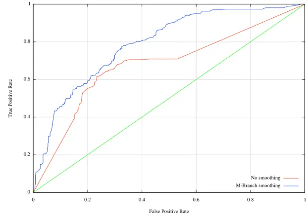
Let us consider the effect of smoothing using a so-called ROC curve (Green & Swets, 1966). Probability estimation methods are often evaluated using ROC curves, which will be discussed in more detail in the next chapter. The larger the area under the ROC curve, which plots true positive predictions against false positive ones, the better the probability estimation method being evaluated. ROC curves are only defined for 2-class problems, where one class is considered negative and the other positive. The area under curve gives the probability that a randomly chosen positive instance receives a higher positive class probability than a randomly chosen negative one.

The plots in Figures 1.2 were generated using the same dataset and the same clas-sifier. The only difference between them is that the red curve is based on no smoothing at all, and the blue curve is based on a technique called M-Branch smoothing discussed later in this thesis. As we can see, the area under the ROC curves is different. Ideally the area in one, which means all positive instances are ranked above all negative ones. Smoothing increases the area under the curve, which is the desired results.

(20)

Figure 1.2: ROC curve with and without smoothing 1.2.2 Cost sensitive classification

Cost sensitive classification is a technique used to minimize the cost of the errors made by classifiers. For example the Weka machine learning workbench (Witten & Frank, 2005) assumes that the errors have the same cost by default, but if a cost matrix is given, it can use this information to pick predictions that minimize the expected cost. In that case, the probability estimates of the classifier are used to calculated the expected cost for each prediction, and the one that minimizes the expected cost is chosen as the final prediction. Cost-sensitive prediction, as opposed to coast-sensitive learning, has the advantage that costs can be varied at prediction time without changing the classifier. However, accurate probability estimates are required for this.

For example, we are trying to classify a patient as having meningitis or not having meningitis, where the estimated probability from the classifier is 0.9 that the patient does not have meningitis. Without any cost on the estimated outcomes, we would classify the patient as “no meningitis” case. However, this is different if the outcomes have costs. If the cost of misclassifying a true meningitis case (false negative) is 100 times higher than the cost of a false positive. The predicted outcome should have the minimum expected cost rather than just the most likely value, which means in this particular case, we classify

(21)

the patient as potentially having meningitis and keep him/her under observation, perhaps performing further medical tests.

1.3

Motivation and Objectives

It is well-known that smoothing techniques can improve the accuracy of class probability estimation. The most basic smoothing method is the so-called Laplace correction (Provost & Domingos, 2003) and it is also implemented in the well-known Weka software. However, there are other more advanced smoothing methods that are not implemented in Weka, such as M-Branch smoothing (Ferri, Flach & Hern´andez-Orallo, 2003). In the field of text compression, there are also some smoothing techniques, and it has not been investigated how well these text compression smoothing methods perform in tree learners. In order to compare smoothing techniques for PETs in Weka, the objectives of this thesis are as follows:

1. Implement the smoothing methods introduced in (Ferri, Flach & Hern´andez-Orallo, 2003) as a state-of-the-art baseline to compare against.

2. Implement the PPM smoothing methods introduced in (Bell, Cleary & Witten, 1990) 3. Run experiments on the different smoothing method implemented

4. Summarize the experiment results and draw conclusions regarding relative perfor-mance.

1.4

Thesis Structure

Chapter 2 will present some background on important concept used in this thesis, such as class probability estimation trees, how to evaluate class probability estimates, and how to blend and adjust probability estimates. In this chapter, the datasets used in the experiments are also introduced and discussed. The data-mining tool Weka will be briefly introduced in this chapter too.

Chapter 3 will describe the different smoothing methods considered in this thesis in depth. Eight kinds of smoothing method will be considered in this chapter: Laplace correction, M-Branch smoothing (Ferri, Flach & Hern´andez-Orallo, 2003) and M-Estimate smoothing (Dzeroski, Cestnik & Petrovski, 1993), and 5 PPM methods: PPMA, PPMB, PPMC, PPMD and PPMP. Note that there are more PPM-related smoothing methods,

(22)

but they are beyond the scope of this thesis. Chapter 3 will discuss the code implemented into one of the tree learners in Weka. The effect on probability estimates will be discussed along with the pseudo code.

The experimental results will be presented in Chapter 4 in tabular and graphical form.

Chapter 5 will summarize the previous chapters, draw conclusions and describe potential future work.

(23)

(24)

Chapter 2

Background and Related work

This chapter discusses background knowledge relevant for this thesis: the basic method for building a class probability estimation tree using information gain and the Laplace correction, building ensemble of trees using bagging, the PPM text compression method, and the datasets and evaluation measures used to evaluate probability estimations in this thesis.

This chapter has the following structure. Section 2.1 introduce the tree learner used in this thesis. Section 2.2 explains the bagging method for ensemble learning. Section 2.3 describes smoothing in PPM text compression. Section 2.4 discusses the datasets used. 2.5 lists and explains different analysis and evaluation techniques.

2.1

Learning Tree Classifiers

The coding done for this thesis was based on Weka (Witten & Frank, 2005). Weka is a collection of state-of-the-art machine learning algorithms and data preprocessing tools. The tree learner used to test and experiment with in this thesis is called REPTree. It is a fast tree learner that uses information gain to find split points and attributes. It is fast because it sorts values for numeric attributes only once. Another reason REPTree is used in this thesis is that it is similar to the tree learner described in the paper by Ferri, C., Flach, P., and Hern´andez-Orallo, J. (2003), which describes the state-of-the-art M-Branch smoothing technique that we will compare to. In this way our results are more comparable with those in the original paper.

There is a simple top-down method for building trees. Information gain is used to decide which attribute is used to split nodes in this process. Higher information gain represents higher purity of child nodes. An impure node has a very mixed distribution of class values. The reason to have a pure child node is that, the more pure the child is, the smaller the subtree is likely to be. The basic algorithm to construct a fully-expanded

(25)

Start on the root of the tree.

If node is not pure or no further splitting is possible:

Find which attribute is the best to split on using information gain Split the node into subsets on possible values

Go to each child node and recurse.

Figure 2.1: Pseudo code for constructing a PET

Start on the root of the tree. If current node is not a leaf node:

Find the split attribute and find the correct path to the child node. Else

return class proabbility distribution

Figure 2.2: Pseudo code for making a prediction using a PET

PET is given in Figure 2.1.

For making a prediction using a PET, we start off at the root node of the tree and check if the node is a leaf node. If it is, then the prediction is over. If it is not, we check the split attribute and find the correction path to go to the child node, then we do the same process recursively until the instance reaches a leaf node. The basic prediction pseudo code for a PET is given in Figure 2.2.

2.1.1 Pruning

Sometimes, a fully-grown tree does not perform as well as a smaller tree. To reduce the vulnerability to noise and variability in the fully grown tree, a process is needed to make the tree smaller and more straight-forward to use. Pruning is a technique that is widely used to reduce a tree to the right size. A pruned tree may not represent a dataset exactly, but a precisely constructed tree does not imply better probability estimates because it may overfit the training data.

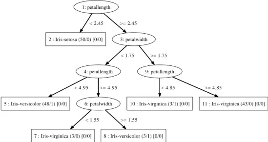
For example, Figure 2.3 shows an unpruned probability estimation tree for the iris data. In contrast to Figure 1.1, the unpruned version of the PET has 11 nodes instead of 5 in Figure 1.1. The right branch from node number 3 (labelled petal width) has been pruned to approximate the unpruned tree. In the unpruned tree, as we can see, after splitting by petal length in node 4 there is a further split on petal width again, which is the same splitting attribute as in node 3.

(26)

1: petallength 2 : Iris-setosa (50/0) [0/0] < 2.45 3: petalwidth >= 2.45 4: petallength < 1.75 9: petallength >= 1.75 5 : Iris-versicolor (48/1) [0/0] < 4.95 6: petalwidth >= 4.95 7 : Iris-virginica (3/0) [0/0] < 1.55 8 : Iris-versicolor (3/1) [0/0] >= 1.55 10 : Iris-virginica (3/1) [0/0] < 4.85 11 : Iris-virginica (43/0) [0/0] >= 4.85

Figure 2.3: Unpruned PET for iris data

Observing the leaf nodes 7 and 8, the instance counts in these two nodes are rela-tively small. If we look at node number 9, we can see that the child nodes under it have the same class: Iris-virginica, which means the split is not necessary to minimize classification error. After pruning, the subtree from node 4 and below becomes a leaf node with class labelIris-versicolor and the instance counts of all the nodes below it are combined. The same process has been done with the subtree attached to node 9 and its child nodes.

Pruning PETs sometimes makes the tree perform better than the original tree. Two general kinds of pruning exist (Witten & Frank, 2005): pre-pruning and post-pruning, where pre-pruning tries to stop unnecessary splits while growing the tree; on the other hand post-pruning grows the entire tree first then tries to prune the tree based on pruning criteria.

Reduced-error pruning (Quinlan, 1987) is a kind of pruning method where we split the data up. Normally two thirds of the data is used to construct the tree and the rest of the data is used to prune the tree by minimizing an error criterion on the pruning data. This method is implemented in the REPTree classifier that is used in this thesis.

2.1.2 Adjusting probability estimates

When the PET is grown, the training dataset used to grow the tree can potentially have zero appearance for an outcome (i.e. class value) at a particular leaf node. Without any

(27)

smoothing methods, this outcome will be assigned a probability of zero, but assigning a zero probability outcome is problematic for probability estimations in real-world problems. This problem is called the zero-frequency problem (Roberts, 1982).

The zero-frequency problem can occur frequently in practice. This is bad because before predictions are made one or more of the outcomes have already been completely eliminated: Even though the event has never happened before, it does not imply it will never happen in the future. To prevent this problem, an adjustment process is necessary, to adjust the probability estimates of the outcomes, so that we do not have the zero-frequency problem. There are many different ways to adjust the probability estimates. For example, the Laplace correction is a simple smoothing method used to solve this problem. It adds 1 to each class count in the leaf nodes, and it thus effectively solves the zero-frequency problem. However, in practice adding one to each class count may cause some other problems, such as over-smoothing the probability estimates, especially when the dataset is small, perhaps becuase the tree has many branches and each leaf node contains a very small number of instances. To solve this problem a smarter way of smoothing probability estimates should be carried out, and several methods will be discussed in the next chapter.

2.2

Bagging trees

In practice, scientific experiments are usually being repeated using the same or a similar set up several times. Scientists then calculate the averaged outcome for a more accurate result. To improve predictive performance in machine learning there are some similar techniques, such as bagging (Breiman, 1996) and boosting (Freund & Schapire, 1996).

Bagging is the technique used in this thesis. As it resamples instances with re-placement to construct trees, it throws some of the old instances out and replaces them with duplicate instances, so that the trees are built based on variants of the same dataset. The algorithm for bagging is given in Figure 2.4

For example, in bagging with 10 iterations, in each iteration a tree is generated, and the data used are generated by sampling with replacement from the full dataset. Each resampled dataset contains the same number of instances as the full dataset.

(28)

Let n be the number of instances in the training data. For each of iterations:

Sample n instance with replacement from training data. Build classifier from subsample.

Figure 2.4: Pseudo code for bagging

For each of the models generated

Calculate the class probability estimates using current model Return the average of all probability estimates

Figure 2.5: Pseudo code for prediction with bagging

At prediction time, for a test case with an unknown class value, the instance actu-ally go traverses all the 10 PETs made from the previous step to get probability estimates from each tree. Then the class probabilities predicted by the 10 trees are averaged to form an overall class probability estimate. This is the standard process when probability estimates are calculated using bagging. The pseudo code for prediction in bagged trees is in Figure 2.5.

2.3

Text compression and PPM

Text compression is another field of study in computer science, but it shares many char-acteristics with machine learning. Its performance is usually measured in terms of com-pression ratio, memory and time used in the process.

2.3.1 PPM

PPM (Cleary & Witten, 1984) stands for Prediction by Partial Matching. It is an adaptive data compression technique based on context modeling and prediction. A technique called blending is used in PPM for solving the zero-frequency problem. As discussed above the zero-frequency problem occurs when an event has not been encountered before: an estimate of probability based on relative frequency will then be zero. This makes predictive compression impossible. PPM combines several predictions into a single over all probability to solve the zero-frequency problem.

In PPM, blending is the name of the type technique known in tree learners as smoothing. The Laplace correction is a simple way of blending an estimated distribution with the uniform distribution. Several different blending methods are used in PPM (for

(29)

# Dataset Size

1 Monks1 556

2 Monks2 601

3 Monks3 554

4 Tic Tac Toe 958

5 Mushroom 8124

6 Wisconsin Breast Cancer 669

7 Kr vs Kp 3196 8 Sonar 208 9 Pima Diabetes 768 10 Vote 435 11 Yeast 1484 12 Hepatitis 155 13 Liver disorders 345 14 Spambase 4601 15 Ionosphere 351 16 Sick 3772 17 Spect 267

Table 2.1: Datasets used in experiments

example, PPMA, PPMB). The only difference between these methods is the way of calculating escape probabilities. In PPM, the blended (i.e. smoothed) probabilities are calculated as follows: p(φ) = m X o=−1 wopo(φ) (2.1)

whereodenotes the order of the context (the analogue of the depth of a node in a PET),

po(φ) is the probability before blending andwois the weight, calculated using the following equation: wo= (1−eo) l Y i=o+1 ei −1≤o < l (2.2)

Where e is called escape probability and calculated differently in different meth-ods. These methods will be discussed further later in the thesis. The probabilityeo gives the probability of escaping from the order-o context to the order-(o−1) context. In a tree,em would be the escape probability associated with a leaf node.

2.4

Datasets

The datasets used in this thesis to test the newly implemented methods are most of the datasets from the paper that introduced M-Branch smoothing (Ferri, Flach & Hern´andez-Orallo, 2003). They are shown in Table 2.1.

(30)

The first three datasets are the monk’s problems. They all have the same attributes, but one of them has noise added in. They have 8 attributes including the class value.

Tic tac toe is a datasets that contains a number of different tic tac toe game boards and the outcome of the game as the class value. It has 10 attributes. The first 9 represent the 9 game board spaces and the tenth is the game result.

The mushroom dataset is a relatively bigger dataset considering both the number of instances and attributes. It has 23 attributes including the class value. The first 22 attributes describe the different appearances of the mushrooms and the class value defines whether it is edible or poisonous.

The Wisconsin breast cancer dataset contains 10 attributes including the class value. It is a purely numeric dataset. The first 9 attributes are the symptoms and the class attribute tells us whether the cancer is benign or malignant.

Kr vs Kp is a chess game dataset. It contains 36 attributes including the class at-tribute. Each instance contains the setup of a chessboard, where white has a king and a rook and black has a king and a pawn. The class attribute shows if white can win at the end of the game.

Sonar has 61 attributes including the class value. The first 60 attributes are read-ings from the sonar, and the class value determines whether the signal the instance corresponds to is a mine or a rock.

Pima diabetes has 9 attributes including the class value. The first 8 attributes are different properties of a patient and the class value is positive or negative.

Vote is the 1984 United Sates Congressional voting record. It has 17 attributes in-cluding a class value, for democrat or republican respectively.

Yeast has 9 attributes. It is a dataset about proteins. The first 8 attributes are different characteristics of the protein, and the class value shows the sequence name of that protein.

(31)

Hepatitis has 20 attributes including the class value, indicating whether the pa-tient is still alive. Other attributes are symptoms and characteristics of the papa-tient.

Liver disorder has 7 attributes. The first 5 attributes are aspects of blood tests that are related to liver disorders. The 6th attribute is the amount of alcohol consumed by the patient per day. The last attribute is the class value, which separates the data into two sets.

Spambase is a spam e-mail database. It has 58 attributes and the class value indi-cates whether the corresponding message is spam or not.

The ionosphere dataset has 35 attributes including a class value of good or bad. This is a radar dataset collected by the system in Goose Bay, Labrador. The first 34 attributes, they represent 17 pulse numbers, with two attributes per pulse.

The sick dataset contains 30 attributes. The first 29 represent different character-istics, symptoms and the medical history of the patient, such as age, sex and pregnancy. The last one is the class value which shows if the patient is sick or not.

The spect dataset contains 23 attributes. The first 22 attributes are diagnostic features of cardiac SPECT images. The class value shows the patient is normal or abnormal.

All of the above datasets have two classes. They were chosen because the tree learner used in this thesis behaves very similarly with binary-class datasets to the one used in (Ferri, Flach & Hern´andez-Orallo, 2003). The aim was to make the end result more comparable.

2.5

Evaluation methods

To measure the performance of the smoothing methods, several different evaluation meth-ods are considered to make sure all aspects of the methmeth-ods are evaluated. The following evaluation measures are used:

• Root mean squared error • Area under ROC curve

(32)

• Entropy gain

2.5.1 Root mean squared error

Mean squared error or MSE is the average squared error between the predicted value and the actual value. Root mean squared error or RMSE is the squareroot of MSE. Root mean squared error is used often to measure precision of estimates. The squared error is also called the quadratic loss (Witten & Frank, 2005).

M SE= 1 n n X j=1 1 k k X i=1

(pji−aji)2 Mean squared error (2.3)

Here, there arentest instances and kclass values. Thepji are the predicted class proba-bilities and the aji are the observed values (either 0 or 1). Taking the square root yields

the root mean squared error.

RM SE =√M SE Root mean squared error (2.4)

2.5.2 Area under ROC curve

ROC stands for receiver operating characteristic. It represents the performance of a classifier without explicit error costs (Witten & Frank, 2005). The horizontal axis is the false positives rate and the vertical axis is the true positives rate, assuming binary classification. The area under the curve (AUC) (Ling, Huang & Zhang, 2003) is the performance measure used in this thesis. For multi-class probability estimation, the AUC value is first calculated for each class in turn, by considering all other classes as the “negative” class, and then the different AUC values are averaged, using weights based on the relative popularity of each class.

To generate an ROC curve from probability estimates for the positive class, the actual class values in the test data are needed. First, the probability estimates for the test instances are sorted in descending order, thus the highest probability comes first. In other words, the earlier the prediction is in the list, the more likely for it to be positive according to the classifier. Then we use the actual class value to find if the predicted probability is accurate. We start from the origin in the plot, and the top of our ranked list, and go up if the predicted value is true, and go right if the predicted value is false. After all the predic-tions are drawn on the coordinate system, a jagged line is formed. That is the ROC curve.

(33)

0 0.1 0.2 0.3 0.4 0.5 0.6 0.7 0.8 0.9 1.0 0 0.1 0.2 0.3 0.4 0.5 0.6 0.7 0.8 0.9 1.0

False positive rate True positive rate

Figure 2.6: Example ROC curves

Figure 2.5.2 shows three ROC curves, which correspond to three different hypo-thetical classifiers. The red curve has the largest area under the curve. The blue curve has a larger area under it than the black line, but the area under it is smaller than the area under the red curve. The black line has a perfect 50% area under it, which is equivalent to a random prediction in a two class dataset.

2.5.3 Entropy gain

Entropy gain is a measure closely related to compression performance. The so-called informational loss for an event with estimated probability p is -log₂p (Witten & Frank, 2005). Ifpis 1 for every predicted value, the model makes perfect predictions and no bits are needed to correct its mistakes. The number of bits needed is given by the informational loss. In Weka, entropy gain is calculated as

EN T ROP Y GAIN = n X j=1 −logPi− n X j=1 −logpi (2.5)

Where Pi is the “default” prediction for the class value of test instance i and pi is the

model’s prediction. The default prediction is an estimate of the prior probability of each class (e.g. 1/3 in the case of the iris data where each type of iris flower is equally likely).

2.6

Summary

This chapter discussed the background knowledge relevant for this thesis. The tree clas-sifier that is used was introduced first, then the algorithm for constructing a PET was presented and explained with pseudo code. Then some further algorithmic techniques

(34)

used in this thesis were discussed, such as pruning and bagging. Thirdly, smoothing was introduced, followed by the Laplace correction as a simple existing PET smoothing method. Then the PPM text compression method was introduced, followed by the differ-ent smoothing methods used by PPM, its equations, and the escape probability calculation method. The dataset used in the experiments in the thesis were listed and described in detail next. Finally, the evaluation criteria where discussed: area under ROC curve, root mean squared error and entropy gain.

(35)

(36)

Chapter 3

Smoothing methods

In this chapter, the different smoothing methods evaluated using PETs are discussed in detail. The first two smoothing methods are the Laplace correction and the M-Estimate smoothing (Dzeroski, Cestnik & Petrovski, 1993). They are very simple methods that are included for completeness. From the third method on, the methods are discussed in more detail. All these methods will be experimented on and analysed in detail in the next chapter.

3.1

Existing smoothing methods in probability estimation

trees

There are many smoothing techniques available nowadays. To choose a method that will fit tree learning well therefore requires detailed experiments and analysis. We now discuss the basic methods that will be evaluated later.

3.1.1 Laplace Correction and M-Estimate

The Laplace correction, the strategy of adding one to each count, will eliminate a 0 count for a predicted outcome. It is the most basic technique for smoothing probability estimates and widely used in practice.

The M-Estimate (Ferri, Flach & Hern´andez-Orallo, 2003) is another commonly used smoothing technique, where M is a constant defined by the user. The Laplace correction and the M-Estimate are defined as follows:

pi= ni+ 1 X i∈C ni ! +c Laplace Correction (3.1) pi = ni+p·m X i∈C ni ! +c M −Estimate (3.2)

(37)

Hereni is the count of instances for classifrom the leaf node concerned,cis the number of

classes. The M-Estimate, if p= 1/m, becomes the formula shown in Equation 3.1, which is Laplace correction. In the experiments with PETs in (Ferri, Flach & Hern´andez-Orallo, 2003), M = 4 is used, because it is the best experimental value.

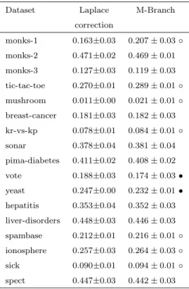
3.1.2 M-Branch Smoothing

M-Branch smoothing is introduced as a new method in (Ferri, Flach & Hern´andez-Orallo, 2003). It is more complicated than the Laplace correction and the M-Estimate because it combines multiple probability estimates. It is defined as follows:

pj_i = n j i +m·p j−1 i X i∈C nj_i ! +m M ₋Branch Smoothing (3.3)

Here mis not just a constant. It varies according to the formula below:

m=M _·(1 + (1₋1/h)_·√N) (3.4)

where M here is a again a user-specified constant as in the M-Estimate, and N is the global cardinality of the dataset. The value his the height of the node in the tree.

According to Equation 3.3, the smoothing method is no longer applied to just the leaf nodes as in the Laplace correction and in M-Estimate smoothing. It smoothes the probability along the path of prediction in a PET based on the probability estimatespj_i for each node j. According to Equation 3.4,mis calculated based onh, the height of the cur-rent node. By observing the equation, it is not hard to find out that if the node is higher up in the tree, it is smoothed more heavily, where the normalised height of a node is 1₋1/h.

The probability of each outcome is fixed at 1/c above the root node, c being the number of possible prediction outcomes. Then we pass that probability to the root node of the PET, calculating the smoothed probability estimate until we reach the leaf node, where the normalized height of the node is 0, thus m=M.

For example in Figure 1.1, we can take the path from the root node to the versi-color node The relevant calculations are shown in Table 3.1.

(38)

Height Node Counts Unsmoothed probability estimates Normalized Height

N Setosa Versicolor Virginica ∆ m

-1 - - 1₃ - 1₃ - 1₃ - -

-3 1 150 ₁₅₀50 50 ₁₅₀50 54 ₁₅₀50 50 2₃ 36.66

2 3 150 0 0 ₁₀₀54 54 ₁₀₀50 50 1₂ 28.50

1 4 150 0 0 49₅₄ 54 ₅₄5 5 0 4.00

Smoothed probabilities 0.00510 0.87676 0.11814

Table 3.1: M-Branch smoothing effects along a path of prediction

3.2

PPM and escape probabilities

In PPM, blended probabilities are calculated using the equation mentioned in the previous chapter in Equation 2.1. In this equation, there is the variable wo, which is the weight of each context In PETs, the context is provided by the path to the current node. The weight is calculated using Equation 2.2, whereeis the escape probability.

The escape probability can be viewed as the probability of “escaping” from the current node to the parent node to determine the prediction for a new test instance, based on the probability that a previously unseen class value is encountered. There are a variety of ways of calculating the escape probability. They are named by combining PPM with the probability method code. PPMA is the PPM method using the escape probability calculation method A.

It is very hard to say which escape probability calculation method is the best of all, or to even make this statement about just two of them, but in practice there is one that is the most suitable one for the problem at hand. The more escape calculation methods there are, the more options we have when we have a problem. In this thesis, 5 of the most popular PPM escape methods are implemented and experimented on.

3.2.1 PPMA

The first escape probability calculation method is method A (Cleary & Witten, 1984). It is a simple calculation:

eo =

1

Co+ 1 (3.5)

In the text compression case, the number of characters we have seen before in the current context o is given by Co. In PETs this will be the total count of instances

(39)

Height Node Counts Unsmoothed probability estimates Weight Escape

Co Setosa Versicolor Virginica wo eo

-1 - - 1₃ - 1₃ - ₃1 - 1.1_×10−6 ₀

3 1 150 ₁₅₀50 50 ₁₅₀50 50 ₁₅₀50 50 0.00018 0.0066 2 3 100 0 0 ₁₀₀50 50 ₁₀₀50 50 0.0180 0.0099

1 4 54 0 0 49₅₄ 49 ₅₄5 5 0.9818 0.0182

Table 3.2: PPMA smoothing effects along a path of prediction

at the node concerned. The probability of seeing a new type of character or a new class value respectively is 1 over the “new” total number of characters or instance count respectively. As Co grows bigger, the escape probability becomes smaller and smaller. In text compression, after a number of characters have appeared in a con-text, the probability of an entirely new character showing up in upcoming text is very low. Similarly, in PETs, after the model has been built with a fair number of in-stances, the probability of seeing an entirely new class value of a particular node decreases.

If the same path used in Table 3.1 is smoothed with PPMA the result is as it is shown in Table 3.2

3.2.2 PPMB

The second escape probability calculation method is method B (Cleary & Witten, 1984). It uses a different approach to calculates the escape probability:

eo = qo

Co (3.6)

Here, qo is the number of different characters that have occurred in the corresponding context context of order o.

In this approach, the number of different characters that have been seen is taken into account in the calculation of the escape probability and it is proportional to the escape probability. That means if fewer different character have been seen before, it is less likely to see a new character in the future.

This technique effectively only takes an observation into account after it has oc-24

(40)

-1 - - 1₃ - 1₃ - ₃1 - 1.48_×10−5 ₀

3 1 150 ₁₅₀50 50 ₁₅₀50 50 ₁₅₀50 50 0.00073 0.02 2 3 100 0 0 ₁₀₀50 50 ₁₀₀50 50 0.0363 0.02

1 4 54 0 0 49₅₄ 49 ₅₄5 5 0.9630 0.037

Table 3.3: PPMB smoothing effects along a path of prediction

curred twice. It is inspired by the consideration that a one-off event may be an error.

In PETs, if fewer classes values have been seen in a node, that means the proba-bility of a new class occurring at this node is low. Vice versa, if a node is relatively less pure, it is more likely that we will see more different classes occurring at this node.

The same path used in Table 3.1 is smoothed with PPMB and the result is shown in Table 3.3

3.2.3 PPMC

The third method is method C (Moffat, 1988). It is similar to method B:

eo = qo

Co+qo (3.7)

This approach is based on the observation that PPMB effectively only takes an observation into account when it has already occurred twice, which seems wasteful. On the other hand, escape probability method A can be problematic, if a context occurs frequently, but with different characters. As a compromise between PPMA and PPMB, PPMC, a hybrid, was introduced. It gets the advantages of both method A and B. Looking at the equation, the only difference is that the denominator has an added value

qo. This will lower the escape probability of the entire context.

In PETs, PPMB has a similar disadvantage: if a node has a small number of in-stances, adding one to the class count will affect the probability estimates dramatically.

(41)

-1 - - 1₃ - 1₃ - ₃1 - 1.37_×10−5 ₀

3 1 150 ₁₅₀50 50 ₁₅₀50 50 ₁₅₀50 50 0.00069 0.0196 2 3 100 0 0 ₁₀₀50 50 ₁₀₀50 50 0.035 0.0196

1 4 54 0 0 49₅₄ 49 ₅₄5 5 0.9643 0.0357

Table 3.4: PPMC smoothing effects along a path of prediction

By using PPMC, we lower the estimated probability of a new a class occurring at the current node.

The same path used in Table 3.1 is smoothed with PPMC and the result is shown in Table 3.4

3.2.4 PPMD

The fourth method is method D (Howard, 1993). It is similar to method B too:

eo = qo/2

Co (3.8)

As in PPMB, if a new symbol occurs for the first time, 1 will be added to qo, as

the number of different characters that have occurred. However, in PPMD, when a new character occurs for the first time, 1/2 is added instead of 1 to the numerator of the escape probability. Thus, as in PPMC, a context will be used even if all observed characters are different.

The same path used in Table 3.1 is smoothed with PPMD and the result is shown in Table 3.5

(42)

-1 - - 1₃ - 1₃ - ₃1 - 1.85_×10−6 ₀

3 1 150 ₁₅₀50 50 ₁₅₀50 50 ₁₅₀50 50 1.83×10−4 _0.01

2 3 100 0 0 ₁₀₀50 50 ₁₀₀50 50 0.01831 0.01

1 4 54 0 0 49₅₄ 49 ₅₄5 5 0.9815 0.0185

Table 3.5: PPMD smoothing effects along a path of prediction

3.2.5 PPMP

The fifth method is method P (Witten & Bell, 1991). It is pretty unique compared to the other escape probability calculation methods. The formula for PPMP is as follows:

eo= n1 Co − n2 C2 o +_{· · ·} (3.9)

As the equation shows, there are different fractions connect by a plus sign or a minus sign, and the plus or minus sign take turns. The numerator of each fraction is the number of classes that has occurred a certain number of times: for example, n1 is the number of

classes that occurred has 1 time in the current node.

Note that here n1 can be 0, but a probability cannot be a negative number. This

problem will be discussed in Section 3.4. When n=Co, and it is the only fraction in the equation, the probability is 1, which should be avoided. However this problem does not happen in this thesis, because it does not occur in the datasets considered.

Differently from all the escape probability calculation methods above, the method is based on an open equation. The number of fractions of the equation is not fixed. However, as the denominater grows exponentially, the later fractions reduce exponentially, and their combination will become insignificant after the 9th or 10th fraction, depending on the number of instances in the dataset. In this thesis, 5 was chosen to be the number of fractions used in the equation because even the smallest dataset, hepatitis, has 155 instances. The denominator will be 89466096875 for the 5th fraction, the result of that fraction is a very small number.

(43)

Setosa Versicolor Virginica PPMA 0.00006 0.89995 0.09997 PPMB 0.00025 0.89223 0.10756 PPMC 0.00023 0.89275 0.10702 PPMD 0.00006 0.89984 0.10010 Table 3.6: Smoothing effects compared

For each item d in the array of class counts d = d+ 1

Figure 3.1: Pseudo code for Laplace correction in REPTree

3.3

Smoothing effects

Several PPM-based smoothing methods and smoothed probability estimates are have been discussed above. All the smoothed probability estimates are shown in Table 3.6 for comparison. By observing the table, notice that the probability estimates of different the methods are very similar. That is because of the characteristics of the iris data, which yields a large and almost pure leaf node..

From the little difference of the probability estimates, we can see that PPMA and PPMD has smaller smoothing effects, which correctly reflects the smoothing effect of Equation 3.8.

3.4

Implementing the smoothing methods

In order to test all the methods described above, the methods have to be implemented into a suitable tree learner. Firstly we have to find a tree learner that is similar to the one used in the literature (Ferri, Flach & Hern´andez-Orallo, 2003). The most suitable tree learner in Weka has been picked out, namely REPTree, a fast decision tree learner that uses information gain.

The simple Laplace correction smoothing has been implemented into REPTree first. The pseudo code is shown in Figure 3.1

Similar to the Laplace correction, the M-Estimate has been implemented in REP-28

(44)

For each item d in the array of class counts d = d + (m · N umber of classes1 )

Figure 3.2: Pseudo code for M-Estimate in REPTree 1 if leafNode

2 return 1

3 else

4 if the attribute is missing

5 Loop through each branch and calculate the height; 6 then combine based on split proportions

7 height = combind height 8 else if nominal attribute

9 height = height of the appropriate child node

10 height++

11 else if attribute is greater than split point 12 //For numeric attributes

13 height = height of the first child node

14 height++

15 else

16 height = height of the second child node

17 height++

18

19 return height

Figure 3.3: Pseudo code for height calculation in REPTree

Tree. The code is very similar. The only difference is the different addition made to the original class counts. In both cases estimated probabilities are then calculated by normalizing the array of class counts. The pseudo code for M-Estimate smoothing is shown in Figure 3.2.

3.4.1 M-Branch Smoothing

Implementing M-Branch smoothing is different from implementing the Laplace correction and the M-Estimate. As it uses the height of the node, the code has to be in the prediction portion of the code instead of the PET building portion of the code. For calculating the height of the node, a simple method has been implemented to do it recursively along the prediction path. This code is shown in Figure 3.4. The “expected” height is used when the instance has a missing value for the node concerned.

The actual code for smoothing the probabilities is in the distributionForInstance()

(45)

1 Get height for current node

2 Let N be total number of instances for current node 3 p = smoothed probabilities from parent node

4 calculate normalized height ∆ = 1 - ( 1 / height ) 5 m = M · (1 + ∆ ·

√

numInstances)

6 foreach raw count ci at node

7 smoothed probability = (ci + m · pi) / (N + m)

Figure 3.4: Pseudo code for M-Branch smoothing in REPTree 1 Let weight = 0

2 Let N be total number of instances for current node 3 get escape probability e for current node

4 weight = (1 - e) · product of escape probabilities from path below 5 foreach raw count c_i at node

6 smoothed probability += (ci / N) * weight

Figure 3.5: Pseudo code for PPM in REPTree

from the two methods above, because in M-Branch smoothing, the height of the current node is needed, and multiple probability estimates are combined. The pseudo code for M-Branch smoothing is in Figure 3.4

3.4.2 PPM Methods

The PPM methods are placed in the same location as M-Branch smoothing as they need similar information, and are also applied recursively. The difference between different PPM methods is in the escape probability calculations, thus there is only one piece of code applying the smoothing to the probability estimates. The pseudo code for this is in Figure 3.5.

The method for returning the product of escape probabilities in Figure 3.5, needed for the calculation in Equation 2.2, is a similar procedure as the get height method for M-Branch smoothing. The pseudo code is in Figure 3.6. Note that it need to be called on the appropriate child node in line 4 of the algorithms in Figure 3.5.

For different escape probability calculation methods, a separate function has been created to detect which escape probability method has been chosen by the user and calculate the escape probability required. The pseudo code for getting the escape probability is in Figure 3.7

(46)

1 Let product = 0 2 if leafNode 3 return 1

4 else

5 if the attribute is missing

6 Loop through each branch and calculate the product; 7 combine products based on split proportions

8 product = combined product 9 else if nominal attribute

10 product = calculate product for child node 11 e = escape probability for current node 12 product = product * e

13 else if attribute is greater than split point 14 //For numeric attributes

15 product = calculate product for the first child node 16 e = escape probability for current node

17 product = product * e

18 else

19 product = calculate product for the second child node 20 e = escape probability for current node

21 product = product * e 22

23 return product

Figure 3.6: Pseudo code for getProduct in REPTree

3.5

Summary

This chapter discussed two simple smoothing methods of PETs first, the Laplace correction and M-Estimate smoothing. These methods are used as baseline methods to test the behaviour of the PET we used. Then the smoothing method from the paper by Ferri, Flach & Hern´andez-orallo (2003) was introduced and explained with the aid of its probability estimate calculation equation. A simple smoothing example with the iris dataset was presented in a tabular form.

Then, each of the PPM smoothing methods were introduced. The difference be-tween the PPM methods is the escape probability calculation method. With the help of equations for the escape probability, the motivation for each escape probability calculation method was discussed. PPMA simply gives the newly occurred character, in the case of PETs, a new instance, one increment on the total count, which is simple enough to understand: after quite a few number characters have been encountered, the probability that a new character shows up is quite low. PPMB takes a different approach, the character probability calculation is inspired by the rule that observations are counted only

(47)

1 Let Escape Probability e = 0

2 Let N be the total count of instances occuring at current node 3 Let q be the number of classes occuring at current node

4 if method A 5 e = 1 / (1 + N) 6 else if method B 7 if (N = 0 or q = 0) 8 return 1 9 e = q / N 10 else if method C 11 if (N = 0) 12 return 1 13 e = q / (N + q) 14 else if method D 15 if (N = 0 or q = 0) 16 return 1 17 e = (q / 2) / N 18 else if method P 19 if (N = 0 or q = 0) 20 return 1

21 if no class occured 1 time in the current node 22 Calculate e as method C

23 for i from 1 to 5

24 get number of classes occured i times n 25 e -= n / Ni · −1i

26

27 return e

Figure 3.7: Pseudo code for getEscProb method in REPTree

if they have happened twice. Thus the escape probability also uses the number of different characters seen so far. PPMC is a compromise between PPMA and PPMB, which gets the advantage of both methods. PPMD has the least smoothing effect on probability estimates, as it only adds half a count to the number of seen characters of the escape probability, classes in the case of PETs, when a new character occurs. PPMP has the most special approach amongst all the PPM methods considered. The number of classes that have occurred exactly ntimes are involved in the calculation of escape probabilities,

n being a natural number which increments by 1 each time. As the denominator of the fractions involved, if the number of classes is 0 for the first fraction, the end result of the calculation will be negative. As probabilities cannot be negative, the escape probability calculation falls back to method C in this case.

Lastly, the pseudo code of all the smoothing methods discussed in this chapter was presented and explained, including the helper methods: getHeight for M-Branch

(48)

smoothing, getProduct for calculating the escape probabilities, and getEscProb to get the correct escape probability calculation method based on user input.

(49)

(50)

Chapter 4

Experiments

This chapter evaluates the different smoothing methods on the datasets discussed in Chap-ter 2. The methodology and experiment setups are discussed in Section 4.1. Section 4.2 evaluates results from the first two setups, using unpruned REPTree without modifica-tions and with the Laplace correction and M-Estimate smoothing. It compares the un-smoothed probability estimates with those un-smoothed by the Laplace correction and the M-Estimate respectively. Section 4.3 evaluates M-Branch smoothing with comparison to the Estimate. Section 4.4 discusses the newly implemented PPM methods with M-Branch smoothing. Bagging unsmoothed trees is discussed in Section 4.5 The effects of bagging trees with the basic smoothing methods are discussed in Section 4.6. Section 4.7 compares the effect of smoothing bagged trees with M-Branch smoothing to bagged unpruned trees. Section 4.8 considers bagged trees with PPM smoothing. Sections 4.9 to 4.12 consider pruned trees. Section 4.13 presents results for a specific case study based on an e-commerce dataset.

4.1

Methodology and Experiment Setups

For ease of comparing the performance of all the smoothing methods implemented in REPTree in Weka (Witten & Frank, 2005), 17 datasets were selected to be used in the experiments. They were listed in Table 2.1. Some of these dataset contain solely numeric attributes or nominal attributes, some contain both nominal attributes and numeric ones, and some contain missing values.

In practice, one dataset will be divided into two subsets, one subset is used to build the PET, and the other one is used to test the PET built from the training subset. The split percentage can be chosen by the experimenter. For example, we can divide the dataset into disjoint 3 parts, where the dataset is divided randomly. Each of the 3 subsets take turns to test the PET built based on the other two subsets. Then the 3 error estimates are averaged to yield an overall error estimate. This is called a

(51)

3-fold cross-validation. The number of subsets we used to divide the datasets up is the number of folds. Sometimes a single cross-validation might not be reliable. Different cross-validations can be performed using the same algorithm, and we can calculate the average of the error estimates. Usually the number of folds in a cross-validation is set to 10, which is found to be the best number to generate an accurate error estimate (Kohavi, 1995). However, in this thesis, a 20 times 5-fold cross-validation is used, because it is the setup used in the paper by Ferri, Flach & Hern´andez-orallo (2003). This way the experimental results are more comparable. The experiments use the paired corrected t-tester (Nadeau & Bengio, 2001) for significance testing with a significance level of 0.05.

4.2

Smoothing effect of M-Estimate smoothing and the

Laplace correction

We first compare unpruned trees to those smoothed with the Laplace correction and the M-Estimate respectively.

4.2.1 Area under ROC curve

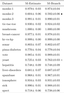
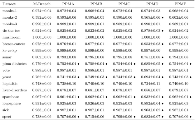
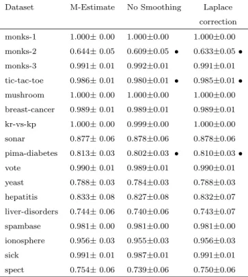
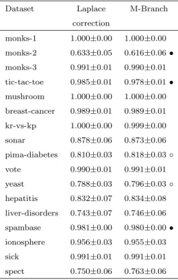
Table 4.1 shows the AUC value from the experiments for REPTree probability estimates with no smoothing versus M-Estimates and Laplace correction. The second column is used as the test base, thus both the third and the fourth columns are compared with the second column. _• in the third column indicates that M-Estimate has significantly improved AUC over the same classifier with no smoothing at all.

In this table, the numbers after the ± are standard deviations. By observing the table, we can see that 10 out of 17 datasets have significant improvements after smoothing with M-Estimate. In face, all the datasets have some improvement with M-Estimate smoothing. In contrast, the Laplace correction has no significant differences compared to M-Estimate smoothing. However, comparing M-Estimate with Laplace correction more closely, it has larger AUC estimates for 6 out of 17 datasets.

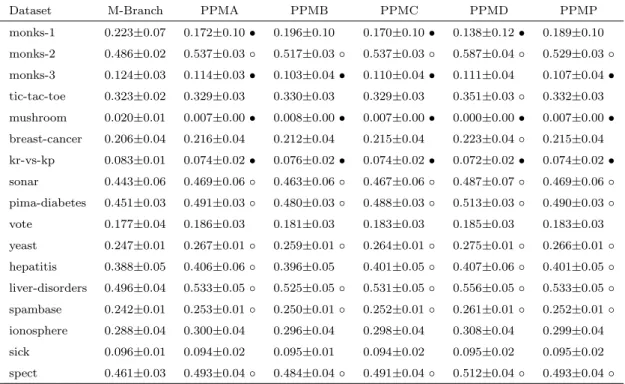
4.2.2 Root mean squared error

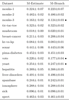
Table 4.2 shows the root mean squared error value from the same experiments as in Table 4.1. Again, the second column is used as the test base, both the third and the fourth columns are compared with the second column. The◦ symbol in the third column indicates M-Estimate smoothing has a significantly smaller root mean squared error

(52)

Dataset M-Estimate No Smoothing Laplace Correction monks-1 0.979±0.03 0.974±0.03 0.980±0.03 monks-2 0.604±0.06 0.568±0.06 • 0.602±0.06 monks-3 0.991±0.01 0.990±0.01 0.991±0.01 tic-tac-toe 0.930±0.02 0.879±0.03 • 0.930±0.02 mushroom 1.000±0.00 1.000±0.00 1.000±0.00 breast-cancer 0.977±0.01 0.952±0.03 • 0.977±0.01 kr-vs-kp 0.999±0.00 0.997±0.00 0.999±0.00 sonar 0.803±0.07 0.751±0.08 • 0.801±0.07 pima-diabetes 0.770±0.04 0.684±0.05 • 0.766±0.04 vote 0.985±0.01 0.984±0.01 0.986±0.01 yeast 0.725±0.03 0.690±0.03 • 0.727±0.03 hepatitis 0.748±0.09 0.717±0.11 0.747±0.10 liver-disorders 0.681±0.07 0.655±0.07 0.680±0.07 spambase 0.968±0.01 0.932±0.01 • 0.967±0.01 ionosphere 0.934±0.03 0.892±0.04 • 0.934±0.03 sick 0.990±0.01 0.965±0.02 • 0.990±0.01 spect 0.718±0.06 0.678±0.07 • 0.711±0.06

◦,•statistically significant difference

Table 4.1: Area under ROC curve

compared to the same classifier with no smoothing. The _• symbol in the third column indicates a significantly bigger root mean squared error. Similarly, the fourth column has the same indicators. In Table 4.2, the Laplace correction improves the probability estimates from no smoothing, and M-Estimate has further improvements from Laplace correction. The raw results in the table also show improvements in most datasets. 11 out of 17 datasets have significant improvements for M-Estimate smoothing over no smoothing and 9 out of 17 datasets have significant improvements for M-Estimates over Laplace correction.

By observing both Table 4.1 and Table 4.2, it is not hard to notice that datasets which do not yield any improvements are similar. These datasets are monks problems 1, monks problems 3, mushroom, kr vs kp and vote. In these 5 datasets, mushroom and

kr vs kp have perfect ROC curves, 100% for mushroom and 99.7% for kr vs kp, which leaves very little potential for improvements. In Table 4.2 the root mean squared error formushroom has increased from 0 to 0.018. This is a typical case of over smoothing.

4.2.3 Entropy gain

Table 4.3 lists the entropy gain for M-Estimate smoothing compared with no smoothing and the Laplace correction, with M-Estimates as the test base. The • symbol in the

(53)

Dataset M-Estimate No Smoothing Laplace correction monks-1 0.224±0.07 0.141±0.12 • 0.188±0.08 • monks-2 0.482±0.02 0.586±0.04 ◦ 0.500±0.02 ◦ monks-3 0.163±0.02 0.122±0.04 • 0.141±0.02 • tic-tac-toe 0.323±0.02 0.351±0.03 ◦ 0.319±0.02 mushroom 0.018±0.00 0.000±0.00 • 0.010±0.00 • breast-cancer 0.211±0.03 0.227±0.04 ◦ 0.214±0.04 kr-vs-kp 0.084±0.01 0.073±0.02 • 0.077±0.02 • sonar 0.441±0.06 0.490±0.07 ◦ 0.456±0.06 ◦ pima-diabetes 0.452±0.03 0.518±0.03 ◦ 0.471±0.03 ◦ vote 0.220±0.02 0.191±0.03 • 0.203±0.03 • yeast 0.254±0.01 0.280±0.01 ◦ 0.256±0.00 ◦ hepatitis 0.389±0.05 0.419±0.06 ◦ 0.396±0.05 ◦ liver-disorders 0.491±0.04 0.559±0.05 ◦ 0.510±0.04 ◦ spambase 0.244±0.01 0.263±0.01 ◦ 0.248±0.01 ◦ ionosphere 0.288±0.04 0.311±0.05 ◦ 0.294±0.04 ◦ sick 0.096±0.01 0.096±0.02 0.095±0.01 spect 0.463±0.03 0.516±0.04 ◦ 0.475±0.03 ◦

◦,•statistically significant difference

Table 4.2: Root mean squared error

third column indicates M-Estimate smoothing has a significantly larger entropy gain over no smoothing. On the other hand, ◦ indicates significantly smaller entropy gain for M-Estimate smoothing. The fourth column has the same indicators for Laplace correction. Table 4.3 also confirms the fact that M-Estimate has the best performance among the three methods: except for mushroom all the datasets exhibit improvements with M-Estimate smoothing. Moreover, 14 out of 17 datasets have significant improvements for M-Estimate smoothing compared to no smoothing. Laplace correction has better performance com-pared to no smoothing at all: 16 out of 17 datasets have improvements with Laplace correction compared to unsmoothed probability estimates, but for 9 out of 17 datasets we prefer M-Estimate smoothing over Laplace correction.

Discussion

In the tables of experimental results, a larger AUC and a smaller root mean squared error and a larger entropy gain are indicators of a better smoothing method. Although there are some significantly degraded experimental results in Tables 4.2 and 4.3, but the over-all results for M-Estimate are better than those for the Laplace correction and the probability estimates before smoothing. The results are quite similar to the results in (Ferri, Flach & Hern´andez-Orallo, 2003), which indicates that the implementation of M-Estimates is correct and that REPTree is similar in behaviour to the classifier used in (Ferri, Flach &

(54)

Dataset M-Estimate No smoothing Laplace correction monks-1 0.68± 0.12 -21.55±27.38 0.75±0.13 ◦ monks-2 -0.01± 0.06 -266.96±50.83•