NBER WORKING PAPER SERIES
A DYNAMIC MODEL OF HOUSING DEMAND: ESTIMATION AND POLICY IMPLICATIONS
Patrick Bajari Phoebe Chan Dirk Krueger Daniel Miller Working Paper 15955 http://www.nber.org/papers/w15955
NATIONAL BUREAU OF ECONOMIC RESEARCH 1050 Massachusetts Avenue
Cambridge, MA 02138 April 2010
The views expressed herein are those of the authors and do not necessarily reflect the views of the National Bureau of Economic Research.
NBER working papers are circulated for discussion and comment purposes. They have not been peer-reviewed or been subject to the review by the NBER Board of Directors that accompanies official NBER publications.
© 2010 by Patrick Bajari, Phoebe Chan, Dirk Krueger, and Daniel Miller. All rights reserved. Short sections of text, not to exceed two paragraphs, may be quoted without explicit permission provided that full credit, including © notice, is given to the source.
A Dynamic Model of Housing Demand: Estimation and Policy Implications Patrick Bajari, Phoebe Chan, Dirk Krueger, and Daniel Miller
NBER Working Paper No. 15955 April 2010
JEL No. D12,E21,R21
ABSTRACT
Using data from the Panel Study of Income Dynamics (PSID) we specify, estimate and simulate a dynamic structural model of housing demand. Our model generalizes previous applied econometric work by incorporating realistic features of the housing market including non-convex adjustment costs from buying and selling a home, credit constraints from minimum downpayment requirements and uncertainty about the evolution of incomes and home prices. We argue that these features are critical for capturing salient features of housing demand observed in the PSID. After estimating the model we use it to simulate how consumer behavior responds to house price and income declines as well as tightening credit. These experiments are motivated by the U.S. recession starting in December of 2007 that saw large falls in home prices, large negative income shocks for many households and tightening credit standards. In the short run, relatively few households adjust their housing stock. Households respond instead by reducing non-housing consumption and reducing wealth because they wish to avoid losing their home and the associated adjustment costs. Households that adjust in the short run are those hit with a series of bad shocks, such as a negative income shock and a home price decline. A larger proportion of households do adjust their consumption in the long run, increasing their housing stock since housing is less expensive. However, such changes may occur several years after the shocks listed above. Patrick Bajari Professor of Economics University of Minnesota 4-101 Hanson Hall 1925 4th Street South Minneapolis, MN 55455 and NBER [email protected] Phoebe Chan Economics Department Wheaton College Norton, MA 02766-2322 [email protected] Dirk Krueger Department of Economics University of Pennsylvania 3718 Locust Walk Philadelphia, PA 19104 and NBER [email protected] Daniel Miller Economics Department Clemson University 222 Sirrine Hall Celmson, SC 29634 [email protected]
1
Introduction
In this paper, we estimate and simulate a dynamic structural model of consumer demand for housing. We use this model to study how housing and non-housing demand will respond to a collapse in home prices, decrease in incomes and a tightening of credit standards. Apart from the direct impact on the housing market, our model has quantitative implications for the size of the wealth effect of house price changes on nondurable consumption expenditures. The evidence can thus shed light on whether the recent decline in home prices triggered a drop in aggregate consumption demand and hence sparked the subsequent recession. Looking forward, our results can serve as predictions for the possible consequences over a longer time horizon.
Over the past decade, housing prices have appreciated at a very fast rate compared to historical standards. Between 1997 and 2006, the nationwide Case Shiller home price index has more than doubled from 84 to 190. The rate of appreciation in certain U.S. cities was much faster than the national average. However, home prices have recently fallen and there is little evidence thus far that there will be a sharp recovery. Between the peak in 2006 Q2 and 2009 Q2 the nationwide index fell 30%. For the most hard hit cities, such as Miami, Detroit, San Diego, Las Vegas, and Phoenix, prices have fallen between 45% and 55% as of June 2009. In addition, due to the sharp decline in economic activity and a subsequent increase in the unemployment rate household incomes have been falling significantly. We will expose households in our model to exactly these house and income declines.
The past two decades have also seen substantial changes in mortgage markets. The tra-ditional 30 year fixed rate mortgage is no longer the standard mortgage product. Since their introduction in the early 1980’s the adjustable rate mortgage had grown to a recent peak of a 40% share of mortgage applications in 2005.1 In addition to adjustable rate mortgages, there has been an expansion of the subprime mortgage market and other non-conforming loans. These credit market innovations helped people with low credit quality become homeowners and also allowed households to buy larger homes. However, it is now clear that the expansion of subprime credit also had a downside. Approximately 15% of subprime loans are in default as of August 2009, three times the rate in 2005.2 As a result, non-conforming mortgages have been more difficult to obtain as lenders have tightened credit in the mortgage market.3 Our struc-tural model is rich enough to trace out, in admittedly stylized way, the consequences for housing and nondurable consumption allocations of a contraction of the availability to households of debt collateralized by housing.
1Source: Freddie Mac annual ARM (adjustable rate mortgage) survey. 2Source: Mortgage Bankers Association.
3According to the 2009 Freddie Mac annual ARM survey, the share of ARM applications is at an all time
In our structural model, a household solves a life cycle dynamic programming problem. In each period, households make investment decisions in housing, choose non-housing consump-tion levels, and make decisions regarding mortgage borrowing and savings. Unlike a typical investment vehicle, housing provides a flow of services that enters utility along with non-housing consumption. We include additional realistic features of housing demand in the model. Ad-justing the stock of housing requires the consumer to incur transaction costs meant to capture realtor fees and other costs related to buying and selling a home. This gives rise to a lumpy pattern in housing investment. The model also includes credit constraints in the form of mini-mum down payment requirements for mortgages. We adopt a partial equilibrium approach by modeling the evolution of income and home prices as exogenous first order Markov processes.
We estimate the structural parameters of our model using household level data on income and housing tenure decisions from the Panel Study of Income Dynamics (PSID). Estimating a fully dynamic model of housing demand is technically challenging; solving the household’s dynamic programming problem is computationally difficult because of two key types of non-convexities. First, housing demand has discontinuities arising from transaction costs to adjust housing stocks. Second, households may face credit constraints because conforming mortgages typically require a 20% down payment. As a result, it is not possible to characterize optimal decisions using Euler equations, nor are we able to use standard GMM methods to estimate the structural parameters.
Instead, we use the multistep method proposed by Bajari, Benkard, Levin (2007) (hereafter BBL) to estimate the model. The first step of BBL requires us to estimate housing decisions rules and the law of motion for the state variables. We use a multinomial logit model of housing investment decisions in the spirit of Han (2010). In each period households either upgrade to a larger home, downgrade, or remain in their existing home. This reduced form model provides a flexible way to capture lumpy patterns in housing investment. We estimate the evolution the exogenous state variables using standard time series and panel econometric techniques. In the second step, we estimate the structural parameters in household utility. The estimator proposed by BBL solves a revealed preference problem. We assume that the policy function estimated for housing investment in the first stage is the solution to a household’s dynamic programming problem. The estimator reverse engineers a period utility function that rationalizes the estimated decision rules by solving a system of revealed preference inequalities. An attractive feature of our estimator is that it allows for non-convex adjustment costs and credit constraints.
Given our parameter estimates, we use our dynamic model to simulate a typical household’s response to a set of negative shocks meant to mimic the current disruptions in the U.S. housing
market. The counterfactuals we consider are a housing price bust, a decrease in income, and a tightening of lending standards. Our results demonstrate that many households do not alter their housing choice in response to these shocks, but rather adjust nondurable consumption expenditures. The intuition behind this result is simple- households in the model only move two to three times before retirement (as do most households in the data). Because they are effectively locked in by the substantial adjustment costs, changes in housing market conditions do not influence their level of housing stock nor housing consumption. Instead, they respond to the shock by partially reducing home equity, partially by reducing expenditures on nondurable consumption goods.
The paper is organized as follows. We review the theoretical and empirical literature relevant for our study in the next section. Section 3 describes the model. Section 4 presents the data and descriptive evidence. In section 5, we provide an overview of the BBL estimation technique. Section 6 and 7 describe the first and second stage of estimation. In section 8 we present our benchmark model simulation results and section 9 conducts sensitivity analysis with respect to crucial structural parameters. Section 10 concludes; additional details about computation are relegated to the appendix.
2
Related Literature
Following Mankiw’s (1982) aggregate study of consumer durables, a sizeable literature has developed that uses structural household-level models of housing demand and tenure choice to study the interaction between house prices, household consumption, and tenure decisions.
The closest paper in spirit to ours is the work by Li and Yao (2007) and Li et al. (2009). The former paper constructs a life cycle model of housing tenure choice to study the impact of house price changes on housing choices and consumer welfare for different age groups of the population. The key distinction between their paper and ours is two-fold. First, while their paper contains a more explicit model of the life cycle and housing tenure choice, they restrict attention to a preference specification in which the elasticity of substitution between nondurables and housing services is fixed to one (that is, the aggregator is of Cobb-Douglas form). Our paper, as Li et al. (2009) estimates this crucial parameter and finds the elasticity to be larger than one. Our model simulations document that this difference has important implications for the dynamics of housing and consumption choices. Second, while their main focus lies on the impact of house price changes on consumption allocations over the life cycle and the distribution of its welfare impacts across different households, we focus more directly on the impact of house price shocks on housing demand and the demand for nondurable consumption.
Li et al. (2009) perform a structural estimation of a model very similar to Li and Yao (2007) using method of moments estimation. The main difference in our econometric method is that we use a multi-step estimator adapted from the dynamic games literature. The advantages of this method compared to brute force approaches are well known. First, there is less risk of misspecification since the first stage is estimated in a completely flexible manner. Second, it is easier to include a rich set of state variables since the model does not need to be computed repeatedly at each point in time. Brute force approaches typically require the researcher to restrict attention to a subset of the relevant state variables of interest because of computational costs. Finally, the computations are often more reliable and accurate. In brute force approaches, numerical error from the inner loop where the model is computed are known to propagate into the outer loop of the optimization procedure. Resulting estimates and standard errors can be very sensitive to the error tolerance in the inner loop and there is no numerical theory to guide these choices. See, for example, Dube, Fox and Su (2009).
Related to our economic model of housing, Flavin and Yamashita (2002), Fernandez-Villaverde and Krueger (2010), Yao and Zhang (2005), Hintermaier and Koeniger (2009), Kiy-otaki et al. (2008), Iacoviello and Pavan (2009). and Diaz and Luengo Prado (2008, 2009) use a similar life cycle model to study the impact of the presence of housing on portfolio choice, precautionary saving and the wealth distribution. The latter authors also employ their model to argue that the current user cost approach to measure price changes for housing services in the consumer price index (CPI) is biased in the presence of owner-occupied housing and house-hold heterogeneity. In a sequence of quantitative papers Chambers, Garriga and Schlagenhauf (2009a,b,c) use a life cycle model with tenure choice to explore the impact of tax treatments and different mortgage designs on home ownership rates and explore the reasons for the substantial increase in this rate in the U.S. in the last decade. Yang (2009) documents the role of down payment constraints and transaction costs on the life cycle profile of housing and consumption. Oralo-Magne and Rady (2006) study the interaction of financial markets conditions and home ownership rates in a structural model of housing choices. Lustig and van Nieuwerburgh (2006) and Piazessi, Schneider and Tuzel (2007) explore the connection between house and asset prices. The role as collateral of housing is the main theme of a recent literature that focuses on the joint housing and mortgage choice. Important examples of this work include Hurst and Stafford (2004), Luengo-Prado (2006), and Chambers et al. (2009a,b). The recent increase in default on mortgages has motivated a small but growing literature on structural models of foreclosures within this context. See, for instance, Jeske et al. (2010) and Garriga and Schlagenhauf (2009). The same issue is analyzed empirically, among others, by Carroll and Li (2008).
consumption from changes in house prices. Leading work in this strand of the literature include Case, Quigley, and Shiller (2003), Benjamin, Chinloy and Jud (2004) and Campbell and Cocco (2007). They document a sizable housing wealth effect and contrast their results to estimates of the wealth effects from other financial assets. We use our model to document how strongly nondurable consumption responds to a house price decline and study how this negative wealth effect from house prices interacts with down payment constraints and negative income shocks. Our paper also contributes to the literature on estimation of dynamic decision problems with non-convex adjustment costs. To the best of our knowledge, the only paper that attempts to estimate such a structural model, besides Li et al. (2009) cited above is Hall and Rust (2003). The simulated minimum distance estimator that they propose is not computationally feasible in our application because it requires repeatedly computing the optimal policy function. Computing a single optimal policy function in our model takes one week of CPU time with an advanced workstation. Our estimator avoids the burden of repeatedly computing optimal policies. Finally, our paper is closely related to Han (2010). Our first stage is quite similar to her reduced form model of housing demand. We depart from her work because we estimate a households structural utility parameters. This allows us to explore counterfactuals that would not otherwise be possible in a reduced form approach.
3
The Model
We model a typical household’s consumption and housing choice as a partial equilibrium, dynamic decision problem with a finite lifetime horizon. Households live for T periods and in each period t they choose consumption expenditures on nondurables, ct,and the amount of
one period-risk free financial assets to bring to the next period, at+1. We let ht denote the
size of the household’s real housing stock at the beginning of the period, so that ht+1 is the amount of housing chosen today for tomorrow. A household derives a service flow g(ht) =ght
from the housing stock where g >0 is a parameter. In our application, we shall assume that g = 0.075, which is close to estimates of housing user costs in the literature. Households value nondurable consumption and housing services according to a standard intertemportal lifetime utility function U {ct, ht}Tt=0 =E0 " T X t=1 βt−1u(ct, g(ht)) +γβT log(bT) # (1)
where β is the standard time discount factor and γ measures the degree of altruism to leave bequestsbT at the end of life. ExpectationsE0are taken with respect to the stochastic processes
driving labor income and house prices, which we specify below. Letpt denote the relative price
of one unit of housing, in terms of the numeraire nondurable consumption good. Housing prices
{pt}T
t=0 follow first order stochastic Markov processes.
At time 0, agents are endowed with initial asset holdings (a0, h0) and one unit of time per period, which they supply inelastically to the labor market to earn labor incomeyt. The labor
income process is composed of two components, a deterministic mean life cycle profileεt(which
incorporates aggregate income growth in the economy as a result of technological progress) and a stochastic component ηt that follows a first order Markov process. Households retire at an
exogenous ageTr and receive a flat pension benefit buntil they die. Thus labor income is given
by
yt =
(
εtηt if t < Tr
b if t≥Tr
We model the two main frictions in the housing market explicitly. First, the stock of housing is subject to nonconvex adjustment costs. Specifically, in order to purchase a home of size ht+1 the household has to spend
ptht+1+ptφ(ht+1, ht)
where ptht+1 is the purchase price of the home and ptφ(ht+1, ht) is the transaction cost a
household has to bear when adjusting the owned stock housing from ht to ht+1. We assume that the function φ takes the form
φ(ht+1, ht) =
(
φ∗(ht+1+ht) if ht+1 6=ht
0 if ht+1 =ht
where the number φ measures the transaction cost. In most of our analysis we shall assume that φ= 0.03., that is, which is representative of real estate fees.4
A second key friction in our model is the requirement for households to acquire (and main-tain) some minimal positive equity share in the house. We assume that the joint choice of financial assets and housing positions satisfies the following collateral constraint:
at+1 ≥ −(1−ξ)ptht+1. (2)
4We do not have direct data on transaction prices. In principle, we could infer them indirectly through
the use of our structural model. However, taking a direct stance on transaction costs will give a more efficient estimate of the remaining model parameters. As we shall show in our policy simulations, our model is able to reasonably match key moments of our data, where transaction costs play a large role. Also, the simulation results suggest that qualitatively, many of our policy conclusions will be robust to a fairly broad range of transaction costs as long as they are sizeable (and as long as the adjustment cost function has the nonconvex form we have specified).
Here ξ ∈ [0,1] is the fraction of the purchase price of the house that has to be paid down at purchase, i.e. (1−ξ) is the fraction of the purchase price that can be financed via a mortgage. In most of our experiments we shall assume that households are able to finance at most 80 percent of their housing purchases through mortgages.5 Also note that as long as ξ ∈ [0,1], households can only borrow against their housing collateral; uncollateralized debt is therefore ruled out by assumption in our model.
Thus the key frictions in the housing market are summarized by the transaction cost φ parameter and the collateral constraint parameter ξ, with φ = ξ = 0 denoting frictionless housing markets. Our simulation exercises will therefore be able to quantify the importance of frictions in the housing market by deducing optimal choices of households under various assumptions on (φ, ξ).
In addition to housing, households can use financial assets to accumulate wealth. These assets yield a constant real interest rate r. If households borrow (subject to the collateral constraints), they face a real mortgage interest rate rm > r. In most of our exercises we
treat interest rates as constant, but we will analyze how the dynamic consumption and asset accumulation choices change with the level of interest rates households face.
Defining
r(a) = (
r if a≥0 rm if a <0
the budget constraint can be written as
ct+at+1+ptht+1+ptφ(ht+1, ht) =yt+ (1 +r(at))at+ptht. (3)
Finally, consumption and housing choices are constrained to be nonnegative:
ct, ht+1 ≥0 (4)
Households maximize (1) subject to the constraints (2),(3) and (4). In the appendix we of-fer further details on the recursive formulation and computation of this partial equilibrium household decision problem.
5This is a typical down payment requirement in conforming mortgages offered by Freddie Mac and
Fan-nie Mae. Our sample extends to the 1997 and predates the explosion in subprime mortgages. A 20 percent downpayment requirement is representative of credit constraints during this time period.
4
Data and Descriptive Evidence
In this section, we discuss our data which primarily comes from the Panel Survey of Income Dynamics (PSID), a national household level longitudinal survey. We then present descrip-tive evidence that motivate our modeling choices. Specifically, we document lumpy housing investment and life-cycle patterns of housing tenure decisions.
From the PSID, we select a panel of households between 1980 and 1993, including only households that own their primary residence. 6 The sample contains 1931 households for a total of 14,556 household-year observations. The key variables are income, value of primary residence, annual mortgage payment, home equity, an indicator of whether the household moved in a given year, and demographic information. We supplement our data with 30 year fixed interest mortgage rates from the Federal Housing Finance Agency.7 We also use the home price index from the Federal Housing Finance Agency, which collects home price information from home sales financed with Fannie Mae and Freddie Mac conventional mortgages. Both series span the years 1975 to 2009. We also impute measures of non-housing wealth and consumption from the Consumer Expenditure Survey (CEX). The CEX data are not reliable for estimation, but are nonetheless informative for descriptive purposes.
4.1
Aggregate Descriptive Evidence
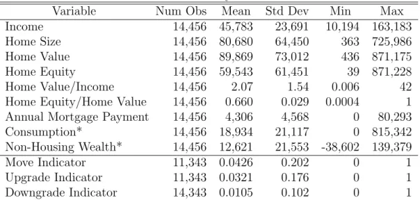
Table 1 lists descriptive summary statistics. All dollar values are deflated by the non-housing component of the consumer price index, which serves as our numeraire good. The base year is 1980. Housing is a significant component of household wealth and expenditures. The average household occupies a $90,000 home, valued at double its annual income. On average households have a 2/3 equity stake in their home, which is by far the largest source of household wealth. Home equity averages $59,000, whereas non-housing wealth reported in the CEX averages $12,000. Households finance 77%, of their home using a mortgage and carry a positive mortgage balance. Annual mortgage payments account for 9% of total income on average.
Adjustment costs to moving play a key role in our model. If the costs are high enough, the model predicts households should move to a different home infrequently and make lumpy adjustments to housing stock. This behavior is evident in the data. Households move in just 4.3% of the years. The size of the adjustments are large, averaging a change of $40,000 in
6We only include households where the head of household is married, between the age of 20 and 65 and born
between 1920 and 1959. We exclude households where the head of household changed during the sample period and any household that reports an income below $10,000 or above $150,000, a trimming of approximately the top and bottom 2% of households based on income. We also exclude a small number of households reporting negative home equity balances.
Table 1: Summary Statistics
Variable Num Obs Mean Std Dev Min Max
Income 14,456 45,783 23,691 10,194 163,183
Home Size 14,456 80,680 64,450 363 725,986
Home Value 14,456 89,869 73,012 436 871,175
Home Equity 14,456 59,543 61,451 39 871,228
Home Value/Income 14,456 2.07 1.54 0.006 42
Home Equity/Home Value 14,456 0.660 0.029 0.0004 1 Annual Mortgage Payment 14,456 4,306 4,568 0 80,293
Consumption* 14,456 18,934 21,117 0 815,342
Non-Housing Wealth* 14,456 12,621 21,553 -38,602 139,379
Move Indicator 11,343 0.0426 0.202 0 1
Upgrade Indicator 11,343 0.0321 0.176 0 1
Downgrade Indicator 14,343 0.0105 0.102 0 1
All dollar values deflated by non-housing component of consumer price index: base year 1980. Move indicator variables reported on a truncated sample size that only includes observations with a non-missing lagged observation.
Home size represents the quantity of housing expressed in 1980 dollars. It is calculated by dividing real home values by the FHFA home price index. We do not have information on household locations and thus are not able to account for regional differences in home prices. * Imputed from Consumer Expenditure Survey
home size. Households typically upgrade to larger homes; 75% of moves are upgrades, with an average increase in home size of $24,000. Table 2 lists the frequencies for the number of moves per household during the 14 year sample period. The majority of households, 58%, never move, and it is rare for a household to move more than once. Extrapolated over a life-cycle, households move one or two times after their first home purchase. Consistent with lumpy investment behavior, the large standard deviation in the ratio of house value to income (1.54 reported in table 1) in part indicates that households do not continuously adjust housing in response to income fluctuations.
4.2
Life Cycle Patterns
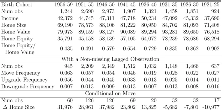
Table 3 reports summary statistics by birth cohort. Several patterns emerge about life cycle behavior.8 Both income and housing exhibit a hump-shaped pattern. Young households move into progressively larger homes until they are middle-aged and in the process accumulate home equity, both in total and as a percentage of home value. But as households approach retirement, income falls and they downgrade to smaller homes. The frequency of moves declines in age, from 6.3% for the youngest cohort to 2.7% for the oldest.
8In general, a cohort table cannot distinguish life cycle effects from cohort effects; life cycle interpretation is
Table 2: Household Moves Number of Moves Frequency 0 58% 1 34% 2 6.5% 3 1.4% >4 0.4% Sample duration 1980-1993.
Note: we may be underreporting the number of moves because of gaps in the panel.
Table 3: Birth Cohort Sample Means
Birth Cohort 1956-59 1951-55 1946-50 1941-45 1936-40 1931-35 1926-30 1921-25 Num obs 1,244 2,690 2,973 1,907 1,321 1,458 1,851 924 Income 42,372 44,745 47,311 47,718 50,234 47,092 45,332 37,690 Home Size 69,190 78,573 88,106 81,222 80,950 84,702 81,093 71,408 Home Value 79,973 89,159 98,127 90,089 89,294 93,281 89,650 76,518 Home Equity 35,791 45,158 58,139 57,105 64,072 78,239 78,686 68,294 Home Equity/ Home Value 0.435 0.491 0.579 0.654 0.729 0.835 0.862 0.902 With a Non-missing Lagged Observation
Num obs 945 2,209 2,349 1,512 1,032 1,148 1,466 637 Move Frequency 0.063 0.057 0.054 0.046 0.019 0.028 0.022 0.027 Upgrade Frequency 0.056 0.044 0.045 0.033 0.013 0.025 0.014 0.011 Downgrade Frequency 0.007 0.013 0.009 0.013 0.007 0.013 0.008 0.016 Conditional on Move Num obs 60 126 126 69 20 32 32 17 ∆ Home Size 31,976 28,961 37,982 23,802 13,825 -5,682 -7,801 -10,977 All dollar values deflated by non-housing component of consumer price index: base year 1980.
5
Estimation Procedure
We use the two-step method proposed by Bajari, Benkard, and Levin (2007) for estimating the structural parameters of our model. The estimation procedure in this paper proceeds in two steps. In the first step, the economist flexibly estimates the reduced form decision rule and law of motion for the state variables. In the model in section 3, the exogenous state variables include income, home prices, and interest rates. Endogenous state variables include the current stock of housing and savings. The decision rule is the optimal choice of housing and savings as a function of the current state.
In the second step, the economist finds the structural payoff utility parameters which ra-tionalize the reduced form decision rules. We model period utility with a familiar constant elasticity of substitution form. During the life cycle households derive utility from housing, h and non-durable consumption c, according to the period utility function,
u(c, h) = logh(θcτ + (1−θ)(κh)τ)1τ
i
whereθ and τ are parameters to be estimated. The term,θ captures consumption shares, and the term τ captures the elasticity of substitution between housing and non-housing consump-tion. The elasticity parameter is particularly important as our counterfactual exercises will demonstrate in the next section. Other models of housing demand (see Li and Yao (2007)) assume this parameter takes on a value of zero (unit elasticity). We set the utility flow of housing parameter toκ= 0.075. This implies that for every $100,000 dollars of housing stock, valued in 1980 dollars, the agent receives $7,500 in housing services for a particular year. This number is consistent with the literature on owners equivalent rent.
In our model, households maximize lifetime expected discounted utility given time t in-formation. In order to simplify our problem, we assume that households live until age 70. Expected discounted can be written as:
Et
70 X
t0=t
βt0−tu(ct0, ht0) +β70−tγlog(q70)
In the above, q70 is the amount of home equity at age 70. Our model allows for a bequest motive where households value leaving housing equity to its heirs. The parameter γ describes a household’s preference to leave a bequest. A bequest motive is necessary to understand observed choices since otherwise agents would have a strong incentive to liquidate all housing att = 70.
6
First Stage: Reduced Form Policy Functions
The first step of Bajari, Benkard, and Levin (2007) requires us to estimate an agent’s reduced form decision rule. The in model of section 2, the choice variables of the agent are next period’s housing stockht+1,non-housing consumption ct and borrowing/savingsat. Our dynamic
pro-gramming model implies that these decisions should be a function of an agent’s state variables. We begin by describing our estimation of ht+1.
In the presence of transactions cost to moving, households move infrequently and, when they do, make lumpy adjustments to their stock of housing. We model this as a mixed discrete/continuous choice problem. The method of Bajari, Benkard, and Levin (2007) requires that we flexibly approximate the agent’s decision rules so that we let the ”data speak” and allow us to empirically recover the decision rules the agents are using. Ideally, one would use non-parametric methods for inference. However, as a practical matter, nonparametric rules do not work well when there are more than 2 or 3 conditioning variables or the number of observations is moderate in size as will be the case in our application. As is well known, the curse of dimensionality in these methods generate very poorly estimated models. In our application, we instead use specifications that are parametric, but allow for flexibility through the inclusion of splines and higher order terms when the data is sufficiently rich.
We use a multinomial logit model. The probability of household i making a moving choice of j at timet is given by pit,j =P[Mit =j] = exp (s0itβj) P3 k=1exp (s 0 itβk) (5) The theoretical model of the last section implies that an agent’s policy function in the dynamic program should depend on the state variables. In the above, we label the state variables as sit. These include variables such as prices, current income, liabilities and housing stock. Since
income follows a life cycle process, we will also want to keep track of individual specific state variables such as age.
We expect households that experience an increase in income to be more likely to upgrade and less likely to downgrade. Households occupying small homes might be more likely to upgrade and less likely to downgrade. To capture the impact of a down payment constraint, we include a linear spline in the home equity ratio. Specifically, we allow the effect of the home equity ratio to differ for equity ratios above and below 15%. If down payment constraints have an important effect on housing decisions we would expect the likelihood of moving—in particular, upgrading—to reduce significantly as equity falls through the lower range. We would expect the equity ratio to have much less effect in the higher home equity range. We apply the user
cost method to measure the price of home ownership. We use a simple measure: the difference in real interest rates and the expected real rate of home price inflation. This measure captures both the financing costs of mortgage interest payments and the offsetting investment component of housing capital gains. In our application, we assume households have rational expectations and thus measure expected home price inflation using the realized value of contemporaneous home price inflation. We also condition on age and age-squared since our model suggests that life cycle considerations should influence housing choices.
We use a parsimonious specification to capture the lumpiness in housing stock adjustments. We model the size of housing stock adjustments as a simple average of log changes in home size:9
|log(hit+1)−log(hit)|=β0+it (6)
Under the assumption that the error term and u error term in the multinomial logit model are uncorrelated, we can estimate the adjustment size separately using the subset of households that either upgrade or downgrade. We have also experimented with more elaborate specification. However, the number of adjustments in our data is a small fraction of the overall observations. Also, in our second step estimates, we will need to forecast individual level housing decisions. The time series literature on forecasting tells us that over-parameterized models typically generate poorer forecasts that more parsimonious specifications. Therefore, we opt for this simple specification.10
6.1
Reduced Form Policy Function Results
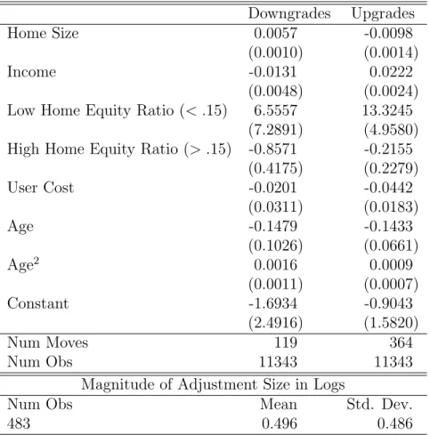
Table 4 reports results for the multinomial logit model. The coefficients on the decision to remain in the current home are normalized to zero. Almost all of the coefficient signs are as expected. Households in larger homes are more likely to downgrade and less likely to upgrade. As income increases, they are more likely to upgrade and less likely to downgrade. As the price of housing increases, measured by the user cost, households are less likely to upgrade. User cost has an insignificant effect on downgrades. We find down payment constraints are quite important. In the low equity range, below 15%, a drop in equity lowers the probability
9We also tested methods that distinguished upward and downward adjustment sizes and parameterized
ad-justment size through factors such as income and home size. We found that such models performed poorly when simulations veered outside the support of the distribution of the variables. Moreover, with so few observations of upgrades and downgrades there is a large loss in degrees of freedom from estimating separate adjustment sizes.
10We also experimented with an (S,s) inventory model of durable good expenditures as in Attanasio (2000).
This model imposes more structure than a flexible multinomial logit. With so few adjustments, the (S,s) model did not yield reasonable results.
Table 4: Upgrade/Downgrade Multinomial Logit Downgrades Upgrades Home Size 0.0057 -0.0098 (0.0010) (0.0014) Income -0.0131 0.0222 (0.0048) (0.0024) Low Home Equity Ratio (< .15) 6.5557 13.3245
(7.2891) (4.9580) High Home Equity Ratio (> .15) -0.8571 -0.2155
(0.4175) (0.2279) User Cost -0.0201 -0.0442 (0.0311) (0.0183) Age -0.1479 -0.1433 (0.1026) (0.0661) Age2 0.0016 0.0009 (0.0011) (0.0007) Constant -1.6934 -0.9043 (2.4916) (1.5820) Num Moves 119 364 Num Obs 11343 11343
Magnitude of Adjustment Size in Logs
Num Obs Mean Std. Dev.
483 0.496 0.486
All dollar values deflated by non-housing component of consumer price index: base year 1980. There is a linear spline in the home equity to house value ratio term with a knot value at 0.15. The reported coefficients are the marginal effects in each region. Standard errors in parentheses. Magnitude of adjustment size measured as|log(hit)−log(hit−1)|for households that move. Sample restricted
to observations with non-missing lagged observations.
of upgrading. The magnitude is very large. Households also less likely to downgrade as equity falls, which makes sense since, even after a downgrade, such households may have difficulty securing a new mortgage. In the high equity range, home equity has no significant effect on upgrades, but extra equity makes it less likely for a household to downgrade. Finally, older households are less likely to make any sort of adjustment.
6.2
Mortgages and Savings
We do not have reliable data on household savings, mortgage choices, and bequests and cannot estimate these decisions from data. We have attempted to make imputations from other data sources, including the CEX, but have found these imputations to be too imprecise and this measurement error appeared to bias our estimates. Instead we make the following parsimonious
modeling assumptions based on what we know about the mortgage and savings decisions of the typical U.S. household during this time period. We assume that households used mortgage products that were common during the 1980’s and early 1990’s.
We assume households finance their homes with 30 year fixed rate mortgages. A household that moves transfers home equity from its prior residence into the new home. The remaining value of the home is financed with a new 30 year fixed rate mortgage set at the prevailing interest rate.11 We also assume housing is only the source of wealth. We abstract from other forms of borrowing or lending. We note that our data from the CEX shows non-housing wealth is insignificant portion of households’ total assets.
In some instances, particularly near the end of the life cycle, a household could have excess home equity. This happens for downgrades to homes valued less than the current amount of home equity. We lock this excess wealth into an annuity with an amortization term that expires at end of the life cycle. Thus, the annuity is completely drained at the end of life cycle. Periodic payments supplement income. Consumption is simply the difference between income and mortgage payments. If a household pays off its mortgage in full, it consumes its entire income. Households do not prepay or refinance mortgages, nor can they borrow against their home equity. These assumptions restrict a household’s ability to draw down home equity to smooth consumption and to save beyond the value of a home in anticipation of a bequest.
We do not directly impose a down payment constraint in our estimation. Instead, we let down payment constraints enter through the equity ratio term in the multinomial logit model of moving decisions. Finally, it is necessary to impose a subsistence requirement. In rare instances simulated consumption would be negative. We endow those households with $1,000 in consumption. Likewise, if home equity is negative at the end of the life cycle, we endow those households with $1,000 in equity for a bequest. Both of these assumptions can be interpreted as an insurance policy against particularly poor shocks.
We must make these assumptions because we do not have reliable data on mortgage fi-nancing and savings. Nonetheless, we feel they are reasonable, and we show that our forward simulations match key moments from the life cycle quite closely.
6.3
Exogenous State Variables: Income, Home Prices and Interest
Rates
In the method of Bajari, Benkard, and Levin (2007), the econometrician must also estimate the stochastic processes governing the law of motion for the state variables. The process for
11The term is 30 years regardless of age. It may be reasonable to assume older households choose shorter
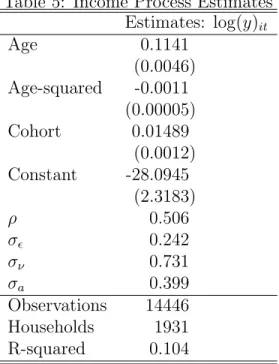
Table 5: Income Process Estimates Estimates: log(y)it Age 0.1141 (0.0046) Age-squared -0.0011 (0.00005) Cohort 0.01489 (0.0012) Constant -28.0945 (2.3183) ρ 0.506 σ 0.242 σν 0.731 σa 0.399 Observations 14446 Households 1931 R-squared 0.104
Random Effects with AR(1) error term dis-turbance. Regressand: log consumption-deflated income. Cohort is the head of household’s birth year. Standard errors in parentheses.
income includes an age component, a cohort effect, household random effects, and an AR(1) error disturbance:
log (yit) = β0+β1ageit+β2age2it+β3birthcohorti +αi+itzit
zit = ρzit−1+νit
it ∼ N(0, σ2)
νit ∼ N(0, σν2)
αi ∼ N(0, σα2) (7)
Estimates are reported in table 5 which shows that income is persistent and exhibits a hump-shaped pattern over the life-cycle.
We model the time series process for real interest rates rt and real home price inflation πt
as a Vector Auto-Regression (VAR) with one lag,
rt = βcr+βrrrt−1+βrππt−1+ert
Table 6: Interest Rate and Home Inflation VAR interest rate home inflation
rt−1 0.615 πt−1 0.534 (0.105) (0.147) πt−1 -0.435 rt−1 0.113 (0.086) (0.178) constant 2.845 constant 0.178 (0.641) (1.090) Error Covariance r 3.399 π 2.543 9.823 Num Yrs 33 1975-2009
Standard errors in parentheses.
where the error term is distributed bivariate normal, e∼N(0,Σ). We use a longer time series that spans the years 1975 to 2009. Results are presented in table 6. Notice the coefficient on the home inflation constant; average real home price inflation was just slightly greater than zero over this time period.
6.4
Goodness of Fit
Using our estimated decision rule and law of motion, it is possible to simulate the entire life cycle of housing decisions for an agent in our model. This simulation is a key input into the Bajari, Benkard and Levin (2007) estimator. We use two methods to evaluate the goodness of the fit of our simulations. First, we examine the entire, 40 year, simulated life cycles for the youngest cohort of households aged 30 to 34. Second, we consider the first five years of forward simulation for all cohorts. In both exercises, we average several key variables across households and simulation paths for five year intervals.
Table 7 reports the full life cycle simulation for the youngest cohort. As a first check, compare the cohorts’ initial conditions in the data column to its first five years of simulations in the “ages 30-34” column. The fit is sensible. Beyond the first five years, the simulated life cycles show a distinct hump shaped pattern in income and consumption. There is also a hump shaped pattern in home size; in early years households upgrade rapidly, then there is a leveling off mid-life, and a slight drop at the tail end of the life cycle. This pattern is largely driven by upgrading and downgrading frequencies. In early years, there is a high rate of upgrades which gradually declines to a low level by the end of the life cycle. Downgrading frequencies are very low and constant up until age 55 at which point they start increasing. A comparison with birth cohort statistics (see table 3) shows that move frequencies match the data quite closely.
Table 7: Forward Simulation for Youngest Cohort Years forward 0 0-5 6-10 11-15 16-20 21-25 26-30 30-35 36-40 Age data 30-34 30-39 35-44 40-49 45-54 50-59 55-64 60-69 65-74 Income 42,372 47,648 55,403 61,975 65,717 66,356 63,457 57,642 54,586 Home Size 69,190 74,992 85,781 95,294 102,767 107,454 109,421 108,678 107,477 House Value 79,973 89,650 111,681 136,486 161,189 184,227 206,344 225,041 231,180 Home Equity 35,791 37,579 47,063 62,420 82,252 106,761 136,716 168,169 179,835 Home Equity/ Home Value 0.435 0.415 0.443 0.494 0.558 0.634 0.721 0.802 0.827 Move Frequency 0.063 0.071 0.063 0.050 0.041 0.032 0.031 0.032 0.034 Upgrade Frequency 0.056 0.060 0.053 0.040 0.030 0.023 0.017 0.012 0.009 Downgrade Frequency 0.007 0.011 0.010 0.010 0.010 0.010 0.014 0.019 0.025 Consumption 43,876 50,608 56,305 59,361 59,588 56,694 51,591 49,118
Non Housing Wealth 308 685 940 1,179 1,644 2,335 3,162 3,359
All dollar values deflated by non-housing component of consumer price index: base year 1980. Italicized entries correspond to the 1956-1959 cohort average in the data. They are aged between 30 and 34. Regular font entries correspond to forward simulations averaged across each 5 year interval.
Although the dollar-valued magnitudes cannot be directly compared, notice that for income and home size the peaks in the hump exactly match the age of the hump in the data. That is, in mid-life (ages 50-54) income peaks, and with a lag (ages 55-59) home size peaks. We also see a steady growth in house values over the life cycle which is partly due to upgrades, and also real home price inflation. In addition, home equity grows as households pay off mortgages and experience home price capital gains. As in the data, we capture an increase in the home equity ratio (home equity/home value) over the life cycle. As a minor point, we include an entry for non-house wealth. This is the size of the annuity from left over home equity for those households that downgrade to homes worth less than their home equity. The magnitude is small, on the order of at most 2% of home equity wealth, and thus the assumptions about non-house savings behavior should have a negligible effect on our final results.
Table 8 reports statistics for each cohort, not just the youngest. Under each cohort heading, the first column reports the statistics from the data, and the second, statistics from five years of forward simulation. Again, the simulations are reasonable. The first five years of simulation are close to the initial conditions and the trajectories of the variables match the hump-shaped patterns that we expect. Young households grow income, housing stocks, and wealth, while older households experience declines. Moving frequencies match quite closely.
Table 8: 5-year Forward Simulation: Birth Cohort
Birth Cohort 1956-59 1951-55 1946-50 1941-45
Data +5yr Sim Data +5yr Sim Data +5yr Sim Data +5yr Sim Income 42,372 47,768 44,745 49,591 47,718 51,420 50,234 50,693 Home Size 69,190 75,097 78,573 83,940 88,106 92,263 81,222 83,857 House Value 79,973 89,611 89,159 99,424 98,127 106,775 90,089 96,701 Home Equity 35,791 37,481 45,158 48,898 58,139 61,934 57,105 60,562 Home Equity Home Value 0.435 0.417 0.491 0.496 0.579 0.581 0.654 0.656 Move Frequency 0.063 0.073 0.057 0.063 0.054 0.048 0.046 0.039 Upgrade Frequency 0.056 0.061 0.044 0.052 0.045 0.039 0.033 0.030 Downgrade Frequency 0.007 0.012 0.013 0.010 0.009 0.009 0.013 0.009 Consumption 43,962 45,630 47,832 47,797
Non Housing Wealth 315 261 273 317
Birth Cohort 1936-40 1931-35 1926-30 1921-25
Data +5yr Sim Data +5yr Sim Data +5yr Sim Data +5yr Sim Income 50,234 52,126 47,092 47,476 45,332 44,514 37,690 36,611 Home Size 80,950 83,060 84,702 86,032 81,093 81,525 71,408 71,399 House Value 89,294 95,397 93,281 98,270 89,650 93,562 76,518 79,982 Home Equity 64,072 67,345 78,239 81,088 78,686 81,120 68,294 70,914 Home Equity& Home Value 0.729 0.729 0.835 0.831 0.0862 0.861 0.902 0.901 Move Frequency 0.019 0.032 0.028 0.026 0.022 0.025 0.027 0.023 Upgrade Frequency 0.013 0.023 0.025 0.017 0.014 0.012 0.011 0.010 Downgrade Frequency 0.007 0.009 0.007 0.010 0.008 0.013 0.016 0.013 Consumption 49,833 46,129 43,647 35,978
Non Housing Wealth 303 539 826 711
All dollar values deflated by non-housing component of consumer price index: base year 1980. “Data” columns represent cohort averages in the data. “+5yr Sim” columns correspond to forward simulations averaged across a 5 year interval. Data columns are blank for consumption and Non Housing Wealth because we do not have data on these variables.
7
Second Stage
7.1
Estimation Details
In this section, we describe the second stage of the estimation procedure that estimates the structural utility function parameters. The method we use to estimate these parameters follows Bajari, Benkard and Levin (2007). For the sake of brevity, we do not explain the entire estimation procedure in this paper, the interested reader is referred to the original paper. In the second stage, the econometrician first simulates life cycle housing and non-durable consumption under the policy function that we estimated in the first stage. Next, he reverse engineers the preference parameters which make this observed policy ”optimal” in the sense that no alternative policies yield higher utility.
There are three types of alternative policy functions in our estimator. The first type draws uniform random perturbations of the multinomial logit model parameters. For the second type, we manually generate variation in moving frequencies and housing shares. Specifically, households move every Nth year, where, for different alternatives, N varies between 3 and 10. In a moving year, households move to a house of size H, which varies across alternatives in a range between 88% and 112% of a household’s initial housing to income ratio. This variation helps to identify housing shares, which depend on both the consumption share θ and elasticity τ parameters. The variation in moving frequencies helps to separately identify the elasticity of substitution. Intuitively, the elasticity determines the length of time that a household would tolerate living in a home that is not optimal. For the third type, we allow households to either deplete or add to home equity in the last five years of the life cycle. In each of those five years, they either convert up to 10% of home equity into consumption or add up to 10% to home equity by reducing consumption. Under the optimal policy they neither add to nor reduce home equity. These alternatives generate variation to identify the retirement/bequest parameter.
7.2
Second Stage Results
We estimate the model on a sub-sample of 450 households. We simulate 55 life cycle paths per household. We use 22 alternative policies with 30% manually generating moving frequency and housing share variation, 70% perturbing policy functions coefficients, and, on top of that, 30% varying end of life home equity. Despite the computational advantages of the method, this is the largest sample that our workstation can accommodate. We use a subsampling procedure to calculate standards. In particular, we estimate the parameters on 100 separate subsamples
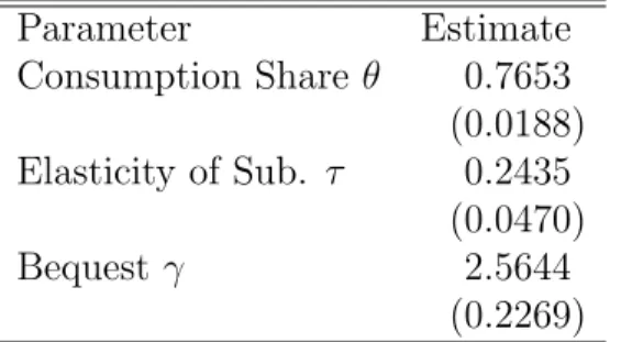
Table 9: Utility Parameter Estimates Parameter Estimate Consumption Share θ 0.7653 (0.0188) Elasticity of Sub. τ 0.2435 (0.0470) Bequest γ 2.5644 (0.2269)
of the same size.12
The results are presented in Table 9. Notice the elasticity of substitution parameter is significantly greater than zero.
As a validation of the results, it is useful to take the estimated parameter results and calculate implied housing shares in a static model of housing demand.13 The implied housing share of income is 17.31%, which compares quite favorably to the 14.3% share in the raw data.
8
Simulation Results from the Structural Model
8.1
Parameterization
In the interest of clarity we summarize the parameters used for the simulations of the structural model in Table 10. Whenever possible and applicable we use the parameters estimated and employed in the previous sections.
We now use these parameters to simulate the response of consumption and asset accumu-lation choices to income and house price shocks. We proceed in three steps. First, in order to briefly explain the main mechanisms of the structural model, we display the life cycle pro-files in the absence of shocks. Then we subject households to joint income and house price shocks, under the benchmark parameterization. Finally we assess the importance of the size of financial constraints, interest rates, and the elasticity of substitution between consumption and housing services in the utility function for household responses to these shocks. The first two sensitivity analyses are motivated by the recent financial and macroeconomic crisis that has led to changes in the extent to which households can borrow against the value of their home and the mortgage interest rates they are able to obtain. The third exercise highlights that precise estimates of structural utility parameters are quantitatively important in assessing
12This procedure does not account for first stage error in the construction of standard errors.
13In the static model, households maximize the period utility function subject to a budget constraint on
Table 10: Parameterization of Structural Model
Parameter Value Interpretation
Preferences
β 0.97 Time Discount Factor
γ 2.56 Degree of Altruism
σ 1 Intertemporal Elasticity of Subst.
g 7.5% Service Flow from Housing Stock
θ 0.77 Consumption Share in Utility Function
τ 0.2435 Elasticity of Sub. between c, h: 1−1τ
Housing and Financial Markets
φ 3% Transaction Cost
ξ 20% Downpayment Requirement
r 1% Return on Financial Assets
rm 7.24% Mortgage Interest Rate
πp 0.95 Persistence of House Price Shock
σp 0.03 Std. Dev of House Price Shock
Labor Income Process
πη 0.95 Persistence of Income Shock
ση 0.3 Std. Dev. of Income Shock
εt= ¯εt(1 +g)t
g = 1.9%
{ε¯t}: Hansen (1991)
Life Cycle Labor Income Profile
the model-implied consumption and wealth response to income and house price shocks.
8.2
The Mechanics of the Model
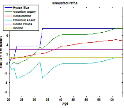
Figure 1 displays life cycle profiles of income shocks14, ηt, and house prices, pt, (the exogenous
stochastic driving forces of the model), consumption of the composite good,ct,financial assets,
at+1,real housing assets,ht+1, and a variable we call voluntary equity,qt+1 =at+1+(1−ξ)ptht+1. As explained in the appendix, it is helpful computationally to use this variable instead of financial wealth in the recursive formulation of the household problem. However, introducing this variable is not only useful for computation, but also helps to interpret the simulation results. Note from the financing constraint (2) it follows that qt+1 ≥ 0, and qt+1 = 0 if the constraint binds. The variable qt+1 measures the equity stake in housing, in excess of the fraction, 1−ξ, as required by the financing constraint. Thusqt+1 = 0 indicates that in periodt households are financing-constrained whereas qt+1 > 0 indicates a non-binding constraint. For the figure (as for all simulations to follow) households start with zero financial and minimal housing assets.15 Underlying the life cycle paths are the decision rules in the presence of income and house price risk, but for this benchmark simulations the realizations of the income and house prices are constant sequences.16
From the figure one can clearly see the key housing market frictions in action. Due to the nonconvex adjustment cost, households alter the size of their houses infrequently: they move three times during the first 15 years of their lives, reaching their desired housing size at age 35 and then, absent further shocks to house prices and incomes, stay put. The fact that households move several times prior to reaching their unconstrained optimal size of the house is due to the presence of the financing constraint. As can be seen from the time path of voluntary equity, after the first move the household’s financing constraint is binding and voluntary equity is zero, qt= 0. After three periods households start to accumulate equity in excess of what is required
from the financing constraint, and another move is triggered. As with the first move, the second house the household purchases is still suboptimally small: after the purchase, voluntary equity is again zero and the financing constraint is binding once again. The households accumulate voluntary equity again until the last upward adjustment in the housing stock occurs once more.
14Recall that total labor income is given byy
t=ηtεt.Thus what we plot here is income net of the deterministic
life cycle component which yields profiles that are easier to interpret.
15We cannot start households off with zero housing since housing purchased today only generates services
tomorrow and the utility function is not well-defined ath = 0. Instead we leth0 =hmin, where hmin is the
smallest point on the housing grid.
16Qualitatively it makes no difference for the dynamics of consumption and housing choices whether the
constant prices and incomes are equal to the low or the high realization of the corresponding Markov chains although quantitatively low house prices and high incomes generate slightly larger and more rapid adjustments in the housing stock position.
Figure 1: Life Cycle Profiles in Absence of Shocks
This last adjustment is “unconstrained” in the sense that the financing constraint is not binding at this move: the household could have afforded a larger home but finds it suboptimal to choose such a larger housing position. In contrast to previous moves, the equity stake exceeds the required minimum share as qt falls following the move but remains positive.
Absent the financing constraint (but in the presence of the nonconvex adjustment cost) households would have moved only once, catapulting them to the optimal size of the house right away. Thus in order to reproduce the stylized fact documented above that households adjust the size of their home infrequently, but more than once on average over their lifetime, the combination of both frictions in the housing market is crucial. Quantitatively the model reproduces the average time in between housing adjustments and the number of moves during a households’ lifetime documented above for US data rather well, at least for the early part of the life cycle.17
Having discussed how households behave in the absence of income and house price shocks we are now prepared to explain how these households, within the model, respond to simultaneous declines in income and house prices as observed recently for the US economy.
17To the extent that the model abstracts from housing transactions triggered by relocation shocks we would
expect the model to understate the frequency with which households move. This is apparent for households in the later stages in their life cycle for which the model, absent income and house price shocks, predicts no housing size adjustments at all.
Figure 2: Life Cycle Profiles with Negative Income Shocks
8.3
Simulating an Income and House Price Shock
The exercise we carry out is intended to mimic a sudden, unlikely, but not entirely inconceivable (from the households’ perspective) decline in the price of housing. At the same time the household receives a negative income shock (which by construction is highly, but not perfectly persistent).18 Given the stylized nature of our structural model, which is necessitated by our desire to estimate it and provide a tight link between theory and estimation, we view our precise quantitative results as less important relative to exhibiting to what extent model elements and parameters (e.g. adjustment costs, the size of the down payment constraint) affect household responses.
In figure 2 we display the life cycle patterns of consumption, housing, and financial wealth prior to and following a negative income shock. We add a concurrent negative house price shock in figure 3. The income (and house price) shock are assumed to hit early in a household’s life, prior to age 35 when the household, in the absence of shocks, would have acquired its optimal housing size (see figure 1).
The key observations we make from both figures is that
18Of course, since we use the decision rule of households derived under the Markov process for income and
prices, households at any period understand that the state of the Markov process can switch with certain probabilty. We simply trace out the dynamic response of households to a particularrealization of the stochastic process.
Figure 3: Life Cycle Profiles with Negative Income Shocks and Negative Home Price Shock
• In response to a negative income shock, households adjust nondurable consumption but do not down size their homes. When the negative income shock hits, households are in the process of moving up the housing ladder and find it suboptimal to (temporarily) downsize.
• The income shock does affect the life cycle profile of housing and nondurable consumption significantly. Relative to the benchmark scenario where households reach their desired stock of housing at age 34, a persistent fall in income delays movements up the housing ladder by a good 16 years (note that this assumes that income falls permanently).19
• While the optimal level and general life cycle profile of housing position is not affected by the fall in housing prices, the timing of the housing adjustments following the shocks is. Specifically, because houses are cheaper now households adjust to their optimal level more quickly, by about 5 years. This suggests the substitution effect dominates the wealth effect of a home price decline.
• The age/equity position at the time when the shock happens is important in determining the household consumption and saving response. If we subject a middle aged household (of age 35 or older) with a large home equity stake to the same shock, this household
19Of course, given that income and house prices are driven by mean-reverting Markov chains, households
finds it optimal to keep its entire life cycle profile of housing unaltered and absorb the entire shock by adjusting nondurable consumption and voluntary equity. A household of this age has accumulated sufficiently many assets (relative to the loss in income over the remaining working life) to keep nondurable consumption reasonably smooth despite the unfavorable income realizations. This result confirms our first stage empirical results showing that age and housing equity are important determinants of housing choices.
• As our results without nonconvex adjustment costs below indicate, the sluggish adjust-ment of the housing position to shocks crucially depends on the imposition of sizeable transaction costs for adjusting the size of houses.
9
Sensitivity Analysis
In this section we perform a sensitivity analysis with respect to three parameters. The first set of comparative statics results is motivated by recent policy relevant changes in the US mortgage market. In particular we want to deduce the impact, within our model, of a tightening of credit lines, as observed in the current crisis of the US mortgage market.
Second we demonstrate that the model with nonconvex adjustment costs on housing gives fundamentally different predictions about household responses to income and house price changes than the frictionless benchmark model of consumer durables (as put forward by Mankiw (1982)) in which the adjustment of the stock of housing is completely costless.
Finally, we have spent considerable effort in precisely estimating the preference parameters of our model, in particular the elasticity of substitution between nondurable consumption and housing services in the utility function. We therefore want to investigate to what extent the results of our model depend on this parameter. To this extent we repeat our simulations with a Cobb-Douglas utility specification which is commonly employed in macroeconomics (see e.g. Fernandez-Villaverde and Krueger (2010) or the discussion in Jeske (2005)).
9.1
Relaxing the Financing Constraint
Our model is rich enough to address the question, albeit in stylized form, of what happens to household’s housing and nondurable consumption decisions as the financial sector tightens credit lines for mortgages. We now draw out the household response to a simultaneous decline of income and house prices under the assumption that households are required to hold only a ξ= 10% equity share of the value of their home as opposed to ξ= 20% as modeled so far. One can interpret our benchmark scenario with tightened credit as the situation after the crisis hit,
Figure 4: Life Cycle Profiles with Relaxed Borrowing Constraints
and the relaxed constraint scenario as the situation prior to the current financial crisis.
Comparing figure 4 to our benchmark results in figure 1 we observe that the main conse-quence of a relaxed downpayment constraint is that households purchase larger homes early in life, and tend to move less frequently. This finding is due to the fact that a relaxed constraint allows households to more quickly trade up in the housing ladder since they can finance more of the purchase price of the house at young ages where they are severely constrained by the collateral constraint. The response to income and price shocks does not depend strongly on the value of ξ, since at the time adjustment after the shock is optimal the financing constraint was not binding anymore even with the tighter financing constraintξ = 20%,see figure 3.
9.2
The Role of Adjustment Costs
The second key friction in the housing market that we model, besides the downpayment con-straint, is the presence of sizable transaction costs that need to be borne if (and only if) households change the size of their home. The benchmark model of consumer durables in macroeconomics abstracts from fixed adjustment costs in the market for consumer durables (see e.g. Mankiw (1982)). Our model nests this specification; by setting the adjustment cost parameter to φ = 0, we obtain the frictionless model.20 In figure 5 we show, in the absence
20Mankiw’s model of a representative consumer did not explicitly include downpayment constraints nor did
Figure 5: Life Cycle Profiles in Absence of Adjustment Costs: No Shocks
of income shocks, that this model delivers fundamentally different predictions for the life cycle profiles of consumption, housing, and financial assets.
Without adjustment costs the model loses its implications derived from lumpy housing investment decision rules. Now the build-up of consumer durables in the early stages of a household’s live proceeds more gradually.21 Note that consumption increases over time since, as long as the household is in debt, the relevant interest rate households face is the mortgage interest rate rm and β(1 +rm)>1.
The model without nonconvex adjustment costs also differs substantially from our bench-mark in the way households respond to income and house price shocks. See figure 6. Now the stock of housing reacts immediately and significantly to the persistent income decline. Nondurable consumption responds as well.22
9.3
The Role of the Elasticity of Substitution
Finally we show that the dynamic consumption and asset choices crucially depend on the key preference parameters which we estimated in previous sections. We now document that
21We solve this version of the model with the same discrete state space dynamic programming techniques as
the benchmark in order to allow for the results to be as comparable as possible.
22Note that the financing constraint remains present in this version of the model. When the shock hits this
constraint is binding and thus a decline in the real value of houses leads to a decline in the value of collateral. Households can borrow less, and consumption of nondurables falls significantly.
Figure 6: Life Cycle Profiles in Absence of Adjustment Costs: Shocks
the optimal choices of households depend on how substitutable nondurable consumption and housing services are in the utility function. Recall that our period utility function was specified as
u(c, d) = 1
τ log [θc
τ + (1−θ) (κh)τ
]
The elasticity of substitution between nondurable consumption and housing services is given by = 1−1τ and was estimated as= 1−01.2435 = 1.32.Rather than going to the extremes of perfect or no substitutability (both of which are highly implausible given our empirical point estimate and the small standard errors around these estimates) we document how our result changes if one adopts the familiar Cobb-Douglas specification23 with unit elasticity of substitution; that is τ = 0 and thus = 1. Conditional on our choice of a unit intertemporal elasticity of substitution σ = 1 this case has the additional appeal that the utility function becomes separable in nondurable consumption and housing services. That is
u(c, d) = θlog (c) + (1−θ) log(κd).
Figure 7 shows that, while qualitatively, the life cycle pattern of consumption and housing response are similar to that in the benchmark case, timing differs. Households adjust their housing stock towards the optimal level more quickly (but to about the same extent) with the
Figure 7: Life Cycle Profiles with Unit Elasticity of Substitution
lower unit elasticity of substitution. Intuitively, the lower the elasticity of substitution, the more costly it is to sustain a suboptimally low housing/nondurables ratio, and thus the more quickly households choose to move up the housing size ladder.
10
Conclusion
In this paper, we have constructed and estimated a dynamic structural model of consumption and housing demand with a frictional housing market. We use our estimated model to simulate counterfactual household responses to a set of negative shocks to income, housing prices, and credit constraints that mimic the current calamity in US housing markets. In our model, we include two key frictions: down payment constraints and non-convex costs to adjust housing stocks. Using household level data from the PSID, we estimate the primitives of the model using the Bajari Benkard Levin (2007) method that is well-suited for estimating such a complicated dynamic model.
Because of the two frictions, nonconvex adjustment costs and financing constraints, house-holds find it optimal to make infrequent housing stocks adjustments. For the benchmark parameterization, households move three times before age 35 as they climb the housing lad-der, before reaching their optimal housing size. Negative income shocks at a young age slow down this accumulation process, but do not induce a downgrade to a smaller home. Adding
a negative home price shock to the negative income shock causes households to move up the housing ladder more quickly because housing is cheaper. As such, any negative effect on home equity wealth is dominated by a substitution effect. The age at which the shocks hit is impor-tant. For older households, having already reached the optimal home size, the negative shocks are absorbed by a reduction in nondurable consumption and home equity. The shocks do not induce a change in housing stock.
We also document the importance of financing constraints, adjustment costs, and the pre-cision of our utility function parameter estimates. All three have significant effects on the frequency of housing stock adjustments and the lumpiness of housing investments. At the center of this adjustment behavior is the ability of households to use home equity to smooth temporary shocks. Future research has to uncover whether introducing further frictions into the housing finance decision that make home equity lines of credit and reverse mortgages less attractive are able to overturn these results.
With regards to a housing market induced recession, our model results suggest there will not be a sudden direct impact on the housing market because adjustments occur with such rarity, and household consumption will be minimally affected by the housing bust because they can use home equity to absorb the shock. Over an extended period of time, the fall in home prices has a mixed effect on housing and consumption allocations. Young households, climbing the housing ladder, benefit from lower home prices in t