Vol.10, No.17, 2018
The Determinants of Emerging Financial Markets Development:
A Case Study of the Dar es Salaam Stock Exchange, Tanzania
Benedicta K. Kamazima1* John Kebaso Omurwa2
1. Graduate Business School, The Catholic University of Eastern Africa (CUEA), P.O Box 62157 - 00200, Nairobi, Kenya
2. The Catholic University of Eastern Africa (CUEA), P.O Box 62157 - 00200, Nairobi, Kenya
Abstract
The stock market plays a vital role in financial intermediation in developed and developing economies (Laichena & Obwogi, 2015). That is because stock markets provide a platform for surplus resources to be transferred to deficit areas. Developing countries lack efficient stock markets like those of the developed countries (Coleman & Tetty, 2008). Therefore, the study sought to investigate the determinants of emerging financial market development using the Dar es Salaam Stock Exchange, Tanzania as a case study. The study had the following specific objectives: to analyze the extent by which market liquidity determines development of emerging financial markets, to establish how inflation rates decides the development of emerging financial markets, to explore how market volatility concludes the development of emerging financial markets and to establish how economic growth determines the development of emerging financial markets. Relevant empirical and theoretical literature was reviewed to inform the objectives of the study and to also form a ground for discussion of results. The study employed a multivariate times series econometric design. The target population of the study included the DSE financial statement data and statistical data from the National Bureau of Statistics, Tanzania. The study used secondary data spanning the period between 2007 and 2016. The data used for the analysis were the monthly figures obtained from the Dar es Salaam Stock Exchange and the National Bureau of Statistics of Tanzania. Diagnostic and model specification tests were done on the data using E-Views version 9. Data was treated for the problem of time series data. To compute forecasts from models with cointegration restrictions, the model is transformed into the VAR levels representation (Brüggemann, 2004). Thus the study used the unrestricted vector autoregressive (VAR) model to do a regression of the dependent variables on the independent variables. The study results were interpreted based on the VAR output. The study concluded that stock market volatility, stock market liquidity and economic growth had a positive and significant long-run relationship with financial market development. Whereas, inflation rates had a negative and insignificant relationship with financial market development. The study recommended that Tanzania relooks at and optimizes its expansionary monetary policy. Policymakers should follow or implement policies which raise macroeconomic stability considering the interaction between economic growth and stock market development.
Keywords: stock exchange, emerging market, market capitalization
1. Introduction
Financial markets play a fundamental role in the economic development of a country. They are the intermediary link in facilitating the flow of funds from savers to investors (Standard & Poor, 2005). By providing an institutional mechanism for mobilizing domestic savings and efficiently channeling them into productive investments, they lower the cost of capital to investors and accelerate economic growth of the country (Seyyed & Paytakhti, 2010). This is only achievable through the growth of stock markets which deal with securities such as stocks thus are associated with financial resource mobilization both on a short and long-term basis (Yartey, 2008).
Economies without well-developed financial markets may suffer from; limited risk diversification; lack of information about the prospect firms whose shares are traded. This has led to the establishment of programs by World Bank, IMF, and ADB for the development of the emerging financial markets in developing countries (World Bank, 2011). The financial market is viewed as a very significant component of the economic growth. Thus, it plays a vital role in the mobilization of capital in many emerging economies (Allahawiah & Al Amro, 2012).
Torre and Schmukler (2014) observed that stock markets in many emerging economies look particularly poor when considering the many efforts already undertaken to improve the macro-economic environment and reform the institutions believed to foster financial development. This disappointing performance has made the conventional policy recommendations for stock exchange development questionable at best. Policymakers are left without explicit guidance on how to revise the reform agenda and a bright future for domestic capital markets specifically for local stock markets or smaller emerging economies (Atje & Boyan, 2013).
The failure to develop deep and efficient stock markets may have important consequences; growing empirical evidence suggests that stock market is not just correlated with a healthy economy; it actually causes economic growth and has a positive impact on poverty alleviation and income distribution. (Daillami & Atkin,
2010; Okereke, 2013). Therefore, a better understanding of the determinants of financial market development and the perceived effects in many emerging economies can provide valuable guidance to boost the development of stock exchange which ultimately contributes extremely to the distribution of income (Singh, 2014).
1.1 Emerging Financial Markets
Based on existing literature, a financial market is defined as a collection of markets that deal with financial assets, including those which pay off in the short term usually less than one year (money market) and whose life is a long-term (known as the capital market) (El-Erian & Kumar, 1995). This is a market where people trade financial securities, commodities at low transaction costs and at prices that reflect supply and demand (Stulz, 2013). Financial markets can also be defined as any marketplace where traders buy and sell stocks, bonds, derivatives, foreign exchange and commodities (Glenn, 2011).
An emerging market is a financial market of a developing country, usually a small market with a short operating history (Osei, 1997). However, as per the International Finance Corporation, an emerging market is one which is found in a developing country (IFC, 2014). Barry and Lockwood (2012) equally define emerging markets as financial markets where the ratio of investable market capitalization to Gross National Product is low.
1.2. The Dar es Salaam Stock Exchange (DSE) in Tanzania
The Dar es Salaam Stock Exchange (DSE) is the securities exchange of Tanzania, one of the fastest growing economies in Africa. The exchange was incorporated in 1996 as a private company limited by guarantee and became operational in 1998. The principal legislation governing the securities industry in the country is the Capital Markets and Securities Act of 1994, amended in 1997, 2000 and 2010. The legislation provides power to the Capital Markets and Securities Authority (CMSA) to be the overall regulator of the DSE and organizations dealing with the securities that trade at the exchange. The first company to list at DSE was Tanzania Oxygen Limited (DSE: TOL) in 1998, which was also the first state-owned company selected for privatization through the capital markets. This was followed by Tanzania Breweries Limited (DSE: TBL), Tanzania Cigarette Company (DSE: TCC), Swissport (DSE: SWIS), Portland Cement (DSE: TPCC), Tanga Cement Company Limited (DSE: TCCL) and National Microfinance Bank (NMB). Following these first state-driven listings, other private companies decided to list at DSE as a part of their corporate growth strategy to raise capital. In 2013, the DSE launched a second-tier market, the Enterprise Growth Market (EGM) with lower listing requirements. The EGM was designed to attract small and medium companies with high growth potential. By 2017, there were twenty-six listed companies at the DSE, ten licensed brokers and three custodian banks.
In 2015, the DSE was demutualized with an aim at maximizing the value of the investment; thus making the exchange the third in Africa to demutualize after the Johannesburg Stock Exchange (JSE) and the Nairobi Securities Exchange (NSE).
In May 2016, the DSE launched its own IPO of 15 million ordinary shares at TZS 500 per share. The IPO raised TZS 35.8 billion from more than 3,000 investors, which is equivalent to 377% in excess of the targeted capital. Following the oversubscribed IPO, the bourse exercised the greenshoe option of 35% to take up an additional TZS 2.6 billion. After exercising the option, the total capital raised from the DSE IPO is TZS 10.1 billion. In July 2016, following the successful DSE IPO, the Tanzanian bourse listed itself on the secondary market under the ticker "DSE".
Selling and purchase of securities at DSE is conducted through an Automated Trading System since December 2006. Trading is conducted Monday to Friday, presently between 10 am and noon. The trading platform is a modern, SWIFT-ready, large area network and multicurrency enabled system. Brokers currently gather on the trading floor to post their orders, but there are immediate plans to activate the wide area network, allowing them to trade from a distant location. Clearing and settlement of transactions are affected electronically through an electronic Central Depository System (CDS) that has been functional since 1999.
1.3. Statement of the Problem
Stock markets in many emerging economies look particularly weak when considering the many efforts already undertaken to improve macroeconomic environment and reform the institutions believed to foster financial development (Torre & Schmuckler, 2014). Despite various measures instituted by the government of Tanzania, such as stock market liberalization, privatization programs and the establishment of supervisory and regulatory bodies such as the Capital Market & Securities Authority (CMSA) in 1994, performance indicators show a relatively poor performance of the DSE. These include low turnover ratio, low market capitalization to GDP ratio and low value of stock traded to GDP ratio (IFC, 2000). However, as foreign aid to Tanzania is declining, the stock market has become an important avenue for accessing and competing for foreign funds. In the light of these developments, it was mandatory to identify and analyze the factors that lead to the development of emerging markets and to suggest necessary policy recommendation. Thus, this study sought to answer the question; what are the determinants of emerging financial market development? Since most of the reviewed
Vol.10, No.17, 2018
studies were carried out in developed markets like USA, England, and Republic of Korea, the study at hand was, however, conducted at the Dar es Salaam stock exchange (DSE) in Tanzania. The fact that Tanzania is a developing country gave the opportunity to test the theories that underlie the concepts of research using developing country data.
1.4 Research Objectives 1.4.1 Main Objective
The main objective of the study was to establish the determinants of emerging financial markets development, a case study focusing the Dar es Salaam Stock Exchange in Tanzania.
1.4.2 Specific Objectives
The specific research objectives that guided the study include:
i) To explore how market volatility determines the development of emerging financial markets
ii) To analyze the extent to which market liquidity determines development of emerging financial markets iii) To establish how inflation rates determine the development of emerging financial markets
iv) To establish how economic growth determines the development of emerging financial markets.
1.5 Research Hypothesis
i) Ho1: Market volatility does not determine the development of emerging financial markets
ii) Ho2: Market liquidity does not determine the development of emerging financial markets
ii) Ho3: Inflation rates do not determine the development of emerging financial markets
iv) Ho4: Economic growth does not determine the development of emerging financial markets
2. Literature Review
The failure to develop deep and efficient stock markets may have important consequences; growing empirical evidence suggests that stock market is not just correlated with a healthy economy; as a matter of fact it causes economic growth and has a positive impact on poverty alleviation and income distribution as well (Daillami & Atkin, 2010; Okereke-Onyuke, 2013). Despite the crucial role that the financial markets play, most of the empirical studies depicted conflicting results. To confirm this; Bridge (2012) found that there was a negative relationship between market capitalization ratio and the overall growth of emerging stock markets. Abbas (2013) study found that there was an insignificant association between CPI and stock market development whereas market capitalization had a significant association with stock market development. It is clear that the studies reviewed showed mixed results.
Tanzania being a developing country gave the opportunity to determine the true phenomenal situation using developing country data. The research therefore aimed at determining the determinants of emerging financial markets development, bringing in dynamics that have developed up to the current period at the Dar es Salaam Stock Exchange.
3. Theoretical Framework
3.1 Modern Portfolio Theory (MPT)
The MPT was developed by Harry Markowitz and published under the title "Portfolio Selection" in 1952. This theory derived the expected rate of return for a portfolio of assets and an expected risk measure. Markowitz demonstrated that the variance of the rate of return was a significant measure of portfolio risk under a reasonable set of assumptions, and he derived the formula for computing the variance of the portfolio. This formula for the variance of the portfolio not only indicated the importance of diversifying your investments to reduce the total risk of a portfolio but also showed how one can diversify effectively. He assumed that most investors want to be cautious when investing and that they want to take the smallest possible risk to obtain the highest possible return, optimizing return to the risk ratio (Persson et al., 2007).
MPT states that it is not enough just to look at the expected risk and return of one stock. By investing in more than one stock, an investor can obtain the benefits of diversification, a reduction in the volatility of the whole portfolio (Markowitz, 1959). According to O'Neill (2000), MPT has important practical applications such as it reduces volatility in a portfolio of individual stocks. Until the time when MPT was invented by Markowitz, investors gave very few thoughts about managing a portfolio or to the concept of risk. Portfolios were constructed randomly. If an investor thought a stock was going up in price, it was added to the portfolio. No other thinking was required or done (Hagstrom, 2001). The essence of MPT is to seek optimization of the relationship between risk and return by composing portfolios of assets determined by their returns, risks, and correlations with other assets. The MPT establishes a framework where, any expected return is constituted of various future outcomes and are thereby risky, and this relationship between risk and return can be optimized through diversification.
3.2. Capital Asset Pricing Model (CAPM)
CAPM was a theory developed separately by William Shape in 1964 and John Lintner in 1965. The CAPM expands the Portfolio theory and establishes a model for pricing all risky assets. The ultimate product, that is, the capital asset pricing model (CAPM), allows an investor to determine the required rate of return for any risky asset. CAPM was developed to explain the behavior of security prices and provide a mechanism whereby investors could assess the impact of the proposed security investment on portfolio overall risk and return. In addition, CAPM provides a significant conceptual framework for evaluating and linking risk and return. An awareness of this trade-off and an attempt to consider risk as well as returns in financial decision making should help managers achieve their objectives (Gitman, 2006). According to Berk and DeMarzo (2007), CAPM assumes that all investors are risk-averse and rational, aiming to maximize their economic utility function. They choose only the portfolios which maximize the expected return with the level of volatility or risk taken. Likewise, the premise is that while choosing between two portfolios with the same expected returns, the investors would go with the one which is less risky or has a lower level of volatility. Secondly, the theory assumes that all investors can buy and sell unlimited amounts of securities at competitive market prices, in other words, trade without any costs for tax or transactions (Tornau & Møller, 2011). They can also lend and borrow without limits at the risk-free interest rate. The CAPM remains popular due to its simplicity and utility in a variety of situations in the financial markets hence still relevant despite the criticisms.
3.3. The Efficient Market Hypothesis (EMH)
The theory was developed by Eugene Fama in 1970. The Efficient Market Hypothesis describes the behavior of a perfect market in which securities are typically in equilibrium, security prices fully reflect available information about the value of the firm and react swiftly to new information. An efficient capital market is one which security prices adjust rapidly to the arrival of new information and, therefore, the current prices of securities reflect all information about the security (Reilly & Brown, 1997). Because stocks are fairly priced, investors need not waste time looking for mispriced securities as there is no way to earn excess profits. It is an investment theory that states that it is impossible to “beat the market’’ because stock market efficiency induces existing share prices to consistently incorporate and reflect all pertinent information.
As stated by the EMH, stocks consistently trade at their fair value on stock exchanges, making it impossible for an investor to either buy undervalued stocks or sell stocks for exaggerated prices. In view of that, it should be impossible to outperform the overall market through expert stock selection or market timing. According to Fama (1976), the capital market is efficient if prices fully reflect all available information in the market. The theory is therefore still applicable to date in the financial markets since its applicability is still evident as most emerging market practitioners still embrace its usage (French, 2013).
4. Determinants of Emerging Financial Market Development 4.1 Stock Market Liquidity
Stock market liquidity can be defined as the speed and ease with which economic agents can buy and sell securities (Yartey, 2008). The stock market turnover ratio is a commonly used proxy for stock market liquidity. The turnover ratio is the value of total shares traded divided by market capitalization. A high turnover ratio may often be an indication of the low cost of the transaction and a higher ratio may represent greater liquidity and market efficiency.
4.2. Stock Market Volatility
Guo (2012) defines stock market volatility as the systematic risk faced by investors who hold a market portfolio. There are two measures of stock market volatility; the standard deviation of annualized returns and the standard deviation of a stock market index’s returns. The main drawback for using the standard deviation of returns is that it assumes that stock market returns are normally distributed (Jones et al., 2004). The study used the standard deviation of the DSE All Share index to measure the stock market volatility of the DSE.
4.3 Inflation Rates
Inflation rate refers to the general and sustained increase in prices of goods and services. In other words, it is when goods get more expensive (Daferighe and Aje, 2009). The measure for inflation rate will be the consumer price index (CPI) which is a measure that examines the weighted average prices of baskets of consumer goods and services. It is calculated by taking price changes for each item in the predetermined basket of goods and averaging them. Frimpong and Oteng (2011) also applied the CPI as a measure of inflation in their study.
4.4 Economic Growth
Economic growth refers to an increase in the capacity of the economy to produce goods and services compared from one period to another. It can be measured in nominal terms, where it is not adjusted for inflation, or in real
Vol.10, No.17, 2018
terms, where it is adjusted for inflation. GDP is the monetary value of all the finished goods and services produced within a country’s borders within a specific period (Mailafia, 2011). GDP is paramount because it gives information about the size of the economy and how an economy is doing (Callen, 2008). Another measure is the lagged GDP. This can be defined as an economic statistic that tends to have a delayed reaction to a change in the economic cycle (Freund & Pagano, 2014).
5. Empirical Review
Bayar (2016) investigated the macroeconomic determinants of stock market development using evidence from Borsa Istanbul. The study investigated the major macroeconomic determinants of stock market development in Turkey during the first quarter of 2005 to the third quarter of 2015 using ARDL cointegration, Toda and Yamamoto (1995) causality test and regression analysis. The study found that both economic growth and stock market liquidity had a positive impact on stock market development in the long run, while inflation had a negative impact on stock market development in the long run. The study concluded that stock market development and economic growth feedback each other and that policymakers should follow or implement policies which raise macroeconomic stability, banking sector development, stock market liquidity considering the interaction between economic growth and stock market development.
KMMCB (2015) conducted a study on macroeconomic factors and stock market development in Sri Lanka. Descriptive statistics and multiple regression analysis methods were used over the monthly data between 2002 and 2014. The stock market turnover was utilized as the proxy of stock market development while inflation volatility, deposit interest rate, lending interest rate, exchange rate volatility and gross domestic production were used as the key macroeconomic factors. The study results indicated that all macroeconomic factors influence the stock market development. More precisely, this was revealed in Sri Lanka that volatile inflation rate and exchange rate together with higher deposit rate curtailed the stock market development. Furthermore, positive optimism generated by the economic growth and the stock market performance during the previous periods tend to boost stock market performance. The study recommended that to develop the Colombo Stock Exchange (CSE), policymakers can implement policies to stabilize the macroeconomic environment and attract more local and foreign investors to CSE.
Laichena and Obwogi (2015) investigated the effects of macroeconomic variables on stock returns in the East African community stock exchange market. On one hand, the broad aim of the study was to identify the effects of macroeconomic variables on stock returns in East Africa. On the other hand, the specific goal of the study was to determine the effects of interest rates on stock returns in East Africa; to find out whether inflation rate impacts on stock returns in East Africa; to establish whether currency exchange rate affects stock returns in East Africa; to assess whether GDP impacts on stock returns in East Africa. A panel data of 3 East African countries, Kenya, Uganda and Tanzania, over 2005 to 2014 was used in the study. Descriptive analysis and panel data regression analysis were applied in the study. From the results, there was a significant relationship between the macroeconomic variables in the study and stock returns in East Africa. The study recommends that policymakers in East Africa should make efforts towards improving the macroeconomic conditions of the region to improve stock returns.
Raza et al. (2015) examined the impact of foreign direct investments and economic growth on stock market development in Pakistan. Annual time series data was used for the period of 1976 to 2011 and was analyzed using cointegration test based on ARDL bounds test and error correction model and rolling window estimation method. The study found that foreign direct investments, remittances, and economic growth had a positive impact on stock market development in the short and long run as measured by stock market capitalization. The study suggested that in Pakistan, investors can make their investment decisions by focusing on the direction of the considered foreign capital inflows and economic growth.
Zhou et al. (2015) conducted a study on the macroeconomic determinants of stock market development in Cameroon. Their study employed the Calderon-Rossell model modified to examine the macroeconomic factors that affect the stock market development. Their findings showed that: stock market liquidity and financial openness depicted by foreign direct investment and private capital flows are vital determinants of stock exchange development in Cameroon. Opposed to the results found in many other African States, economic growth and the banking sector development did not have a positive and significant impact on the Stock Market development of Cameroon. The study concluded that mainly, Stock Market liquidity (Stock Market Value Traded Ratio) and Financial Openness (Foreign Direct Investment and Private Capital Flows) have a positive and significant influence on the Stock Market development in Cameroon.
Fang et al. (2012) conducted an evaluation of the effect of stock market volatility on stock market growth in South Korea. The study covered the period from 2005 to 2010. They employed GARCH-M model to establish the effect of stock market volatility in stock market growth. The study mainly found out that stock market volatility negatively affected the development of the stock market. The study, therefore, concluded that stock market volatility had a significant negative relationship with the development of stock markets during that
period.
6. Methodology 6.1 Research Design
The research design is a comprehensive plan for data collection in an empirical research project. It is a "blueprint" for empirical research aimed at answering specific research questions or testing specific hypotheses (Neuman, 2002). The study used a multivariate times series econometric design. This is because the study used monthly time series data spanning a period from 2007 to 2016 to establish the relationships among the current and past values over time. A time series is a continuous sequence of observations on a population, taken repeatedly (normally at equal intervals) over time (Bernal et al., 2017). The research design was preferred because it is useful in describing changes over time, keeping track of trends and forecasting future short-term trends.
6.2 Population of the Study
The target population is that population to which a researcher wants to generalize the results of the study (Neuman, 2002). The target population of the study was the DSE financial statement data and statistical data from the National Bureau of Statistics of Tanzania from 2007 to 2016.
6.3 Method of Data Collection and Analysis
Data collection is gathering empirical evidence to gain new insights into a situation and answer questions that prompt undertaking of the research (Kothari, 2004). The study utilized secondary data sources. Secondary data is defined as the data that have already been collected and recorded by someone else and readily available from other sources (Yin, 2003). The secondary data was obtained from the financial statements of the DSE. Statistical secondary data was collected from the National Bureau of Statistics.
Diagnostic and model specification tests were done on the data using E-Views version 9. Data was treated for the problem of time series data. To compute forecasts from models with cointegration restrictions, the model is transformed into the VAR levels representation (Brüggemann, 2004). Thus the study used the unrestricted vector autoregressive (VAR) model to do a regression of the dependent variables on the independent variables. Results were interpreted based on the VAR output.
7. Research Findings
The following section presents the findings and discussion of the results about the determinants of emerging financial markets development, a case study of the Dar es Salaam Stock Exchange.
7.1 Descriptive Statistics
Trochim (2006) contends that, along with simple graphics analysis, descriptive statistics virtually forms the basis of every quantitative analysis of data. Descriptive studies can yield rich data that lead to crucial recommendations. The study used descriptive statistics to provide: means, maximum, minimum and standard deviation of data collected on the determinants of emerging market development, a case of the Dar es Salaam stock exchange.
7.1.1 FMD Series
Figure 1: FMD Series Descriptive Statistics 0 4 8 12 16 20 24
1.0e+14 2.0e+14 3.0e+14 4.0e+14 5.0e+14
Series: FMD Sample 2007M01 2016M12 Observations 120 Mean 2.35e+14 Median 2.13e+14 Maximum 5.36e+14 Minimum 5.60e+13 Std. Dev. 1.58e+14 Skewness 0.448934 Kurtosis 1.687620 Jarque-Bera 12.64255 Probability 0.001798
Vol.10, No.17, 2018
Figure 1 shows that the minimum and maximum values of the FMD series were TnSh 5.36 x10 14 and TnSh 5.60 x 10¹⁴ respectively. The Jarque Bera test statistics test the null of normality against an alternate of non-normality in the series. The Jarque Bera test statistic is 12.64255 with a p-value of 0.001798 which is less than 5% significance level and therefore significant. We, therefore, reject the null hypothesis of normality at 5% significance level in favor of the alternate of non-normality. From the skewness value of 0.448934, we conclude that the FMD data series is positively skewed.
7.2.2 SMV Series
Figure 2: SMV Series Descriptive Statistics
Figure 2 shows that the minimum and maximum values of the SMV series were 0 and 156.3693 respectively. The Jarque Bera test statistic is 420.7525 with a p-value of 0.00000 which is less than 5% significance level and therefore significant. We, therefore, reject the null hypothesis of normality at 5% significance level in favor of the alternate of non-normality. From the skewness value of 2.535215, we conclude that the SMV data series is positively skewed.
7.2.3 SML Series
Figure 3 SML Series Descriptive Statistics
Figure 3 shows that the minimum and maximum values of the SML series were 5.42 x10 -6 and 0.000331 respectively. The Jarque Bera test statistic is 188.3613 with a p-value of 0.00000 which is less than 5% significance level and therefore significant. We, therefore, reject the null hypothesis of normality at 5% significance level in favor of the alternate of non-normality. From the skewness value of 2.158198, we conclude that the SML data series is positively skewed.
0 10 20 30 40 50 60 70 0 20 40 60 80 100 120 140 160 Series: SMV Sample 2007M01 2016M12 Observations 120 Mean 18.42375 Median 4.268484 Maximum 156.3693 Minimum 0.000000 Std. Dev. 28.43011 Skewness 2.535215 Kurtosis 10.64469 Jarque-Bera 420.7525 Probability 0.000000 0 4 8 12 16 20 24 0.00000 0.00005 0.00010 0.00015 0.00020 0.00025 0.00030 Series: SML Sample 2007M01 2016M12 Observations 120 Mean 6.03e-05 Median 3.60e-05 Maximum 0.000331 Minimum 5.42e-06 Std. Dev. 6.84e-05 Skewness 2.158198 Kurtosis 7.363596 Jarque-Bera 188.3613 Probability 0.000000
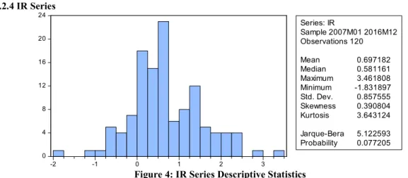
7.2.4 IR Series
Figure 4: IR Series Descriptive Statistics
Figure 4 shows that the minimum and maximum values of the IR series were -1. 18318975 and 3.461808 respectively. The Jarque Bera test statistic is 5.122593 with a p-value of 0.077205 which is more than 5% significance level and therefore insignificant. We, therefore, fail to reject the null hypothesis of normality at 5% significance level and conclude that the IR data series is normally distributed.
7.2.5 EG Series
Figure 5: EG Series Descriptive Statistics
Figure 5 shows that the minimum and maximum values of the EG series were 383,037.6 and 1,428,155 respectively. The Jarque Bera test statistic is 23.10476 with a p-value of 0.000010 which is less than 5% significance level and therefore significant. We, therefore, reject the null hypothesis of normality at 5% significance level in favor of the alternate of non-normality. From the skewness value of 1.019334, we conclude that the EG data series is positively skewed.
7.2.6 Lagged EG Series
Figure 6: Lagged EG Series Descriptive Statistics
0 4 8 12 16 20 24 -2 -1 0 1 2 3 Series: IR Sample 2007M01 2016M12 Observations 120 Mean 0.697182 Median 0.581161 Maximum 3.461808 Minimum -1.831897 Std. Dev. 0.857555 Skewness 0.390804 Kurtosis 3.643124 Jarque-Bera 5.122593 Probability 0.077205 0 2 4 6 8 10 12 14 400001 600001 800001 1000001 1200001 1400001 Series: EG Sample 2007M01 2016M12 Observations 120 Mean 726713.9 Median 687515.3 Maximum 1428155. Minimum 383037.6 Std. Dev. 234881.4 Skewness 1.019334 Kurtosis 3.681748 Jarque-Bera 23.10476 Probability 0.000010 0 2 4 6 8 10 12 14 400001 600001 800001 1000001 1200001 1400001 Series: EG(-1) Sample 2007M01 2016M12 Observations 119 Mean 725959.1 Median 684783.0 Maximum 1428155. Minimum 383037.6 Std. Dev. 235728.3 Skewness 1.026144 Kurtosis 3.673088 Jarque-Bera 23.13029 Probability 0.000009
Vol.10, No.17, 2018
Figure 6 shows that the minimum and maximum values of the lagged EG series were 383,037.6 and 1,428,155 respectively. The Jarque Bera test statistic is 23.13029 with a p-value of 0.000010 which is less than 5% significance level and therefore significant. We, therefore, reject the null hypothesis of normality ` at 5% significance level in favor of the alternate of non-normality. From the skewness value of 1.026144, we conclude that the lagged EG data series is positively skewed.
7.3 Stationarity Tests
The stationary tests were done using the Augmented Dickey-Fuller (ADF) test. The ADF tests the null hypothesis of a unit root (that is the data is not stationary) against the alternate of no unit root (stationarity).
7.3.1 FMD Series
Table 1: FMD Unit Root Test
Null Hypothesis: FMD has a unit root
t-Statistic Prob.*
Augmented Dickey-Fuller test statistic -0.833179 0.8057 Test critical values: 1% level -3.486551
5% level -2.886074
10% level -2.579931
From table 1 the ADF t-test statistic of -0.833179 has a probability of 0.8057 which is more than all the significance levels and therefore we fail to reject the null hypothesis of a unit root in in FMD and conclude that the FMD series is not stationary at level. Further analysis by differencing shows that the FMD series is integrated of order one, I (1).
7.3.2 SMV Series
Table 2: SMV Unit Root Test
Null Hypothesis: SMV has a unit root
t-Statistic Prob.*
Augmented Dickey-Fuller test statistic -1.654499 0.4517 Test critical values: 1% level -3.487046
5% level -2.886290
10% level -2.580046
From table 2 the ADF t-test statistic of -1.654499 has a probability of 0.4517 which is more than all the significance levels and therefore we fail to reject the null hypothesis of a unit root in in SMV and conclude that the SMV series is not stationary at level. Further analysis by differencing shows that the SMV series is integrated of order one, I (1).
7.3.3 SML Series
Table 3: SML Unit Root Test
Null Hypothesis: SML has a unit root
t-Statistic Prob.*
Augmented Dickey-Fuller test statistic -2.351457 0.1579 Test critical values: 1% level -3.487550
5% level -2.886509
10% level -2.580163
From table 3 the ADF t-test statistic of -2.351497 has a probability of 0.1579 which is more than all the significance levels and therefore we fail to reject the null hypothesis of a unit root in in SML and conclude that the SML series is not stationary at level. Further analysis by differencing shows that the SML series is integrated of order one, I (1).
7.3.4 IR Series
Table 4: IR Unit Root Test
Null Hypothesis: IR has a unit root
t-Statistic Prob.*
Augmented Dickey-Fuller test statistic -5.463792 0.0000 Test critical values: 1% level -3.486064
5% level -2.885863
10% level -2.579818
From table 4 the ADF t-test statistic of -5.463792 has a probability of 0.000 which is less than all the significance levels and therefore we reject the null hypothesis of a unit root in IR in favor of no unit root and conclude that the IR series is stationary at level and integrated of order zero, I (0).
7.3.5 EG Series
Table 5: EG Unit Root Test
Null Hypothesis: EG has a unit root
t-Statistic Prob.*
Augmented Dickey-Fuller test statistic -2.503062 0.1176 Test critical values: 1% level -3.492523
5% level -2.888669
10% level -2.581313
From table 5 the ADF t-test statistic of -2.503062 has a probability of 0.1176 which is more than all the significance levels and therefore we fail to reject the null hypothesis of a unit root in in EG and conclude that the EG series is not stationary at level. Further analysis by differencing shows that the EG series is integrated of order two, I (2).
7.3.6 EG Series
Table 6: Lagged EG Unit Root Test
Null Hypothesis: EG(-1) has a unit root
t-Statistic Prob.*
Augmented Dickey-Fuller test statistic -2.439847 0.1334 Test critical values: 1% level -3.493129
5% level -2.888932
10% level -2.581453
From table 6 the ADF t-test statistic of -2.439847 has a probability of 0.1334 which is more than all the significance levels and therefore we fail to reject the null hypothesis of a unit root in in EG (-1) and conclude that the EG (-1) series is not stationary at level. Further analysis by differencing shows that the EG (-1) series is integrated of order two, I (2).
From the ADF tests, it can be seen that one series is I (0), two series are I (1) and two are I (2). This implies that these variables cannot be cointegrated together. Thus, regression analysis cannot be applied to the data.
7.4 Serial Correlation Test
The serial correlation test was based on the residues of the OLS estimate. The Breusch-Godfrey Serial Correlation LM Test tests the null of no serial correlation against the alternate of the presence of correlation.
Table 7: Breusch-Godfrey Serial Correlation LM Test
F-statistic 56.39797 Prob. F(1,112) 0.0000
Obs*R-squared 39.85415 Prob. Chi-Square(1) 0.0000
From table 7 the Breusch-Godfrey F-test statistic of 56.39797 has a probability of 0.000 which is less than all the significance levels and therefore we reject the null hypothesis of a no serial correlation in the residuals against the alternate of the presence of serial correlation in the residues and conclude that the series residues have a serial correlation. Problems of serial correlation imply that the data has either to be treated of serial
Vol.10, No.17, 2018
correlation problems or use a different model altogether.
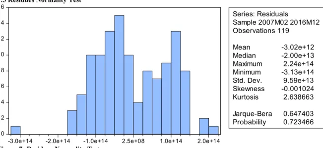
7.5 Residues Normality Test
Figure 7: Residues Normality Test
From figure 7 the Jarque Bera test statistic is 0.647403 with a p-value of 0.723466 which is more than 5% significance level and therefore insignificant. We, therefore, fail to reject the null hypothesis of normality at 5% significance level and conclude that the residues series is normally distributed. The assumption of normality for the use of regression analysis is obeyed.
7.6 Heteroscedasticity Test
The Breusch-Pagan-Godfrey test of heteroscedasticity tests the null hypothesis of homoscedasticity against the alternate of heteroscedasticity (absence of homoscedasticity).
Table 8: Breusch-Pagan-Godfrey of Heteroscedasticity
F-statistic 0.645366 Prob. F(5,113) 0.6656
Obs*R-squared 3.303822 Prob. Chi-Square(5) 0.6533
Scaled explained SS 2.485519 Prob. Chi-Square(5) 0.7787
From table 8 the Breusch-Pagan-Godfrey F-test statistic of 0.645366 has a probability of 0.6656 which is more than all the significance levels and therefore we fail to reject the null hypothesis of a homoscedasticity in the residuals and conclude that the series residues have no heteroscedasticity. The absence of heteroscedasticity implies the use of regression analysis to analyze the data but this is subject to all the other assumptions of the OLS being obeyed.
7.7 Multicollinearity Test
Multicollinearity was tested by using the variance inflation factor (VIF).
Table 9: VIF Test of Multicollinearity
Coefficient Uncentered Centered
Variable Variance VIF VIF
C 2.34E+27 29.81431 NA SMV 1.15E+23 1.688765 1.183740 SML 1.91E+34 2.012761 1.136741 IR 1.17E+26 1.802366 1.089810 EG 1.58E+15 11.83041 1.095225 EG(-1) 1.56E+15 11.60065 1.098071
From table 9 the VIF Test of Multicollinearity shows that the centered VIFs for all the variables are below 4
0 2 4 6 8 10 12 14 16
-3.0e+14 -2.0e+14 -1.0e+14 2.5e+08 1.0e+14 2.0e+14
Series: Residuals Sample 2007M02 2016M12 Observations 119 Mean -3.02e+12 Median -2.00e+13 Maximum 2.24e+14 Minimum -3.13e+14 Std. Dev. 9.59e+13 Skewness -0.001024 Kurtosis 2.638663 Jarque-Bera 0.647403 Probability 0.723466
(generally taken as the critical value) and we, therefore, conclude that the data has no problem of multicollinearity. The absence of multicollinearity implies the use of regression analysis to analyze the data but this is subject to all the other assumptions of the OLS being obeyed.
7.7 Cointegration Test
Engle-Granger cointegration test tests the null hypothesis of no cointegration against the alternate of cointegration.
Table 10: Engle-Granger test of Cointegration
Null hypothesis: Series are not cointegrated
Value Prob.* Engle-Granger tau-statistic -2.685417 0.9310 Engle-Granger z-statistic -16.93529 0.8602
From table 10 the p-values of the test statistics are more than all the significance levels and therefore insignificant. We thus fail to reject the null and conclude that the series are not cointegrated. The absence of cointegration implies that VECM cannot be used to measure either the short run or long run relationships amongst the variables but instead an unrestricted VAR model needs to be applied.
7.8 Unrestricted VAR Model Output
The Unrestricted Vector Autoregressive Model requires specification of the number of lags. To determine the number of lags a VAR of residuals has to be run at each lag level to determine the lag at which the residuals have no serial correlation.
Table 11: VAR Residual Serial Correlation LM Tests
Lag LogL LR FPE AIC SC HQ
0 -1229.421 NA 2575.621* 22.04323* 22.16459* 22.09247* 1 -1324.852 -180.6383 22135.11 24.19379 24.92196 24.48923 2 -1466.264 -255.0456 433313.0 27.16542 28.50040 27.70707 3 -1376.624 153.6679* 137530.3 26.01115 27.95293 26.79899 4 -1396.285 -31.94926 309195.2 26.80867 29.35726 27.84271 5 -1391.709 7.027181 454567.0 27.17338 30.32878 28.45363 6 -1380.567 16.11602 600539.0 27.42085 31.18306 28.94730 7 -1380.190 0.511854 974096.0 27.86054 32.22956 29.63319 8 -1377.377 3.567047 1537119. 28.25673 33.23255 30.27558 The VAR residual serial correlation tests the null hypothesis of no serial correlation against the alternate of the presence of serial correlation. From table 11, using the LM-Stat and the associated probabilities it can be seen that the optimum lag length is 0 (FPE, AIC, SC, and HQ). Therefore, the unrestricted VAR was run by using 0 lags.
Vol.10, No.17, 2018
Table 12: Unrestricted VAR Model Output
FMD C 9.93E+13 (3.3E+13) [ 2.96489] SMV 2.30E+12 (3.4E+11) [ 6.83406] SML 6.64E+17 (1.3E+17) [ 5.02697] IR -7.96E+12 (1.1E+13) [-0.75349] EG -3.70E+09 (7.3E+08) [-5.05222] EG(-12) 3.94E+09 (7.5E+08) [ 5.21791] R-squared 0.670391 Adj. R-squared 0.654233
From table 12, the lagged EG was given a maximum lag of 12 because the data was monthly. All the variables (FMD, SMV, SML, IR, EG, lagged EG) were given a lag of zero (see table 4.12) in running the U-VAR. At 5% and 5 degrees of freedom, the critical value of the t-test statistic is ± 2.57. Thus at 5% significance level coefficient of SMV is significant as its t-value of 6.83406 is more than the critical value. Thus, the finding on objective one is that SMV had a positive and significant long-run relation with FMD. The second objective was to determine the effect of stock market liquidity on financial market development. SML had a positive coefficient with a t-value of 5.02697 which was significant at 5% significance level. Thus, on objective two the study found that SML had a positive and significant long-run relation with FMD. The third objective was to determine the effect of IR on FMD. IR had a negative coefficient with a t-value of -0.75349 which was insignificant at 5% significance level. Thus, on objective three the study found that IR had a negative and insignificant long-run relation with FMD. The fourth objective was to determine the effect of EG on FMD. EG, as measured by real GDP, had a negative coefficient with a t-value of -5.05222 which was significant at 5% significance level while lagged EG as measured by lagged GDP had a positive coefficient with a t-value of 5.21791 which was significant at 5% significance level. Thus, on objective five, the study found EG had a positive and significant long-run relationship with FMD. The model shows that the adjusted R-squared for the VAR is 65.423392% indicating that the VAR model was a good fit for the data.
Table 13: Granger Causality Test
Dependent variable: FMD
Excluded Chi-sq df Prob. Decision Conclusion
SMV 0.235179 1 0.6277 Fail to reject null SMV does not Granger cause FMD SML 2.138400 1 0.1437 Fail to reject null SML does not Granger cause FMD IR 0.417190 1 0.5183 Fail to reject null IR does not Granger cause FMD EG 79.51025 1 0.0000 Reject null EG Granger Causes FMD EG(-12) 79.65709 1 0.0000 Reject null EG(-12) Granger causes FMD
From table 13 the Granger causality test shows that SMV, SML and IR do not Granger cause FMD, while, EG and lagged EG Granger cause FMD.
7.9 Discussion of Findings
7.9.1 Stock Market Volatility and Financial Market Development
The study established that stock market volatility had a positive and significant long-run relationship with financial market development. These results are contradictory to the findings of Fang et al. (2012) who conducted an evaluation of the effects of stock market volatility on stock market growth in South Korea and concluded that stock market volatility had a significant negative relationship with the development of stock markets. Antonios (2010) also concluded that there was negative association between volatility and stock market development. DeLong et.al. (1989) argue that excess volatility in the stock market can hinder investment, and therefore growth. Demirguc-Kunt and Levine (1996) support the study findings by claiming that “greater volatility (in the stock market) is not necessarily a sign of more or less stock market development. Indeed, high volatility could be an indicator of development.
7.9.2 Stock Market Liquidity and Financial Market Development
The study found that stock market liquidity had a positive and significant long-run relationship with financial market development. The results supported by Bayar (2016) who also found that stock market liquidity had a positive impact on stock market development. El-Nader and Alraimony (2013) who investigated the fundamental determinants of stock market development in Jordan also discovered that stock market liquidity had a positive impact on stock market development. Past literature such as Ikikii and Nzomoi (2013) also support the study findings by arguing that the more liquid the markets are, the better, given that liquid markets may make participants take on more risk with an assumption that they can liquidate their positions quickly and at moderately predictable prices. Garcia and Liu (1999) also support the findings by arguing that without liquid stock markets less investment may occur to the high-return projects. Several studies have revealed that market liquidity brought about by the monetary policy has a weaker impact on financial market development (see Lerskullawat, 2017), which could explain the dissimilarities in the research findings with other studies which found a negative relationship.
7.9.3. Inflation rates and Financial Market Development
The study found that inflation rates had a negative and insignificant long-run relationship with financial market development. These findings are supported by KMMCB (2015) who concluded that inflation rate curtailed the stock market development in Sri Lanka. The findings are also supported by Vena and Finance (2014) who stated that high inflation leads to an increase in interest rates leading to decrease in investment activity and ultimately the stock market growth. Fama (1981) supports the study findings by showing that the inverse relationship between real stock returns and expected inflation is generated by a positive relationship between the equity market and the output growth, combined with a negative relationship between expected inflation and real economic activity (the proxy hypothesis).
7.9.4 Economic Growth and Financial Market Development
The study discovered that economic growth as measured by Real GDP had a negative and significant long term relationship with financial market development, while economic growth as measured by lagged GDP had a positive and significant long-run relationship with financial market development. The study concluded that economic growth had a positive and significant long-run relationship with financial market development. These findings are supported by Raza et al. (2015) who examined the impact of foreign direct investments and economic growth on stock market development in Pakistan and concluded that economic growth had a positive impact on stock market development in the short and long run. The findings were however contrary to those of Zhou et al. (2015) who found that economic growth did not have a positive and significant impact on the stock market development in Cameroon. An argument by Siegel (1998) explaining the lack of observable correlation between GDP growth and stock market development is that expected economic growth is already impounded into the prices, thus lowering future returns.
8. Conclusion
Following the study findings on the determinants of emerging financial market development, a case of the Dar es Salaam Stock Exchange in Tanzania, it is concluded that stock market plays an important role in financial intermediation in developed and developing economies (Laichena & Obwogi, 2015). That is, stock markets provide a platform for surplus resources to be transferred to deficit areas irrespective of the economic development of the country in question. To achieve strong financial market economy, economic planners and government leaders in countries where Stock Exchanges offer a combination of short and long-term trading terms to customers, need to pay critical attention to stock market volatility, stock market liquidity, inflation rates and economic growth (both measured by Real GDP and lagged GDP).
Vol.10, No.17, 2018
8.1 Policy Recommendations
Based on the findings of the study, the researcher recommends the following policy actions.
To promote stock market development, emerging market countries can encourage investments by appropriate policies. The policymakers should also consider reducing impediments to stock market development by alleviating restrictions on international capital flows. Researches have shown that market liquidity brought about by the monetary policy has a weaker impact on financial market development. Thus the study recommends that Tanzania relooks at and optimizes its expansionary monetary policy.
Policymakers should follow or implement policies which raise macroeconomic stability considering the interaction between economic growth and stock market development. The government should aim to grow the country’s GDP as it positively influences financial market development. The growth of the GDP can be attained through the initiation of policies that foster growth and development.
8.2 Areas for Further Research
Due to limited time and resources, the study could not exhaust the subject on the determinants of emerging financial market development. The study was confined to the Dar es Salaam stock exchange. Hence, further research could be conducted to include all the East African countries to compare different factors affecting financial market growth in the East African Community countries.
Closely related to the current topic of study, the researcher suggests that further research be done on areas such as the effect of exchange rates on financial market development, the effect of money supply on the financial market development and the effect of capital inflows on the financial market development. Further research should also incorporate behavioral factors to establish whether they affect financial market development. Further empirical studies can also focus on the interaction channels between stock market development and economic growth to see how these two variables affect each other in detail. Further research could advance this study by extending the data sampling period.
References
Abbas, F. (2013). Linking financial development, economic growth, and energy consumption in Pakistan. Renewable and Sustainable Energy Reviews, 44, 211-220.
Allahawiah, S., & Al Amro, S. (2012). Factors affecting stock market prices in Amman Stock Exchange: A survey study. European Journal of Business and Management, 4(8), 236-245.
Antonios, A. (2010). Financial Development and Economic Growth a Comparative Study between 15 European Union Member–States. International Research Journal of Finance and Economics, 35, 143-149.
Atje, R. & Boyan, J. (2013). “Stock Markets and Development,” European Economic Review 37 (2/3), pp. 632-40.
Barry, S. C., & Lockwood, C. M. (2012). Coping with the lionfish invasion: can targeted removals yield beneficial effects?. Reviews in Fisheries Science, 20(4), 185-191.
Bayar, Y. (2016). Macroeconomic Determinants of Stock Market Development: Evidence from Borsa Istanbul.
Financial Studies, 20(1), 70-89.
Berk, J., & DeMarzo, P. (2007). Corporate finance. Pearson Education.
Bernal, J. L., Cummins, S., & Gasparrini, A. (2017). Interrupted time series regression for the evaluation of public health interventions: a tutorial. International journal of epidemiology, 46(1), 348-355.
Bridge, S. (2012). Understanding enterprise: entrepreneurship and small business. New York: Palgrave Macmillan.
Brüggemann, R. (2004). Model reduction methods for vector autoregressive processes (Vol. 536). New York: Springer Science & Business Media.
Callen, T. (2008). What is Gross Domestic Product? Finance & Development, 48-49.
Coleman, A.K. & Tetty, K. (2008). Impact of Macroeconomic Variables of Ghana Stock Exchange. Journal of Risk and Finance, 4, 365-378.
Daferighe, K., & Aje, N. (2009) Empirical analysis of effects of inflation on aggregate stock prices in Nigeria: 1980-2012. European Journal of Accounting, Auditing and Finance Research, 3(9), 31-51.
Dailami, M., & Atkin, M. (2010). Stock Markets in Developing countries: Key issues and Research Agenda’’. Pre-working Paper Series WPS 515, The World Bank Washington D.C.
De Long, J. B., Shleifer, A., Summers, L. H., & Waldmann, R. J. (1989). The size and incidence of the losses from noise trading. The Journal of Finance, 44(3), 681-696.
Demirgüç-Kunt, A., & Levine, R. (1996). Stock market development and financial intermediaries: stylized facts.
The World Bank Economic Review, 10(2), 291-321.
El-Erian, M., & Kumar, M. S. (1995). Emerging stock markets in Middle Eastern countries. In World Bank Conference on Stock Markets, Corporate Finance and Economic Growth, Washington DC, February (pp. 16-17).
El-Nader, H. M., & Alraimony, A. D. (2013). The macroeconomic determinants of stock market development in Jordan. International Journal of Economics and Finance, 5(6), 91.
Fama, E. F. (1981). Stock returns, real activity, inflation, and money. The American Economic Review, 71(4), 545-565.
Fama, E. F. (1976). Agency Problems and the Theory of the Firm. Journal of political economy, 88(2), 288-307. Fang, K., Sung, B. C., & Miller, T., (2012). Mass data analysis and forecasting based on cloud computing on
financial development. Journal of Software,7(10), 2189-2195.
French, S. D. (2013). Evaluation of a theory-informed implementation intervention for the management of acute low back pain in general medical practice: the implement cluster randomized trial. PLoS One, 8(6), e65471. Freund, W.C. & Pagano, M.S. (2014). Market efficiency in specialist markets before and after automation. The
Financial Review 35, 79-104.
Frimpong, G., & Oteng, B. (2011). Modelling Stock Returns Volatility: Empirical Evidence from Saudi Stock Exchange. International Research Journal of Finance and Economics, 85, 166-179.
Garcia, V. F., & Liu, L. (1999). Macroeconomic Determinants of Stock Market Development. Journal of Applied Economics, 2(1). 29-59.
Gitman, D. M. (2006). Symmetries and physical functions in general gauge theory. International Journal of Modern Physics A, 21(2), 327-360.
Glenn, D. W. (2011). Can Financial Market Policies Reduce Income Inequality? Technical Papers Series, MSM-112. Washington, DC: Inter-American Development Bank.
Guo, S. (2012). Propensity score analysis: Statistical methods and applications (2nd Edition). Thousand Oaks,
CA: Sage Publications.
Hagstrom, R. G., 2001, The Essential Buffet: Timeless Principles for the New Economy. New York: John Wiley & Sons.
IFC. (2014). Islamic finance and financial inclusion: measuring use of and demand for formal financial services among Muslim adults. Review of Middle East Economics and Finance, 10(2), 177-218.
IFC. (2000). What matters for financial development? Capital controls, institutions, and interactions. Journal of development economics, 81(1), 163-192.
Ikikii, S. M., & Nzomoi, J. N. (2013). An analysis of the effects of stock market development on economic growth in Kenya. International Journal of Economics and Finance, 5(11), 145.
Jones, C. P., Walker, M. D., & Wilson, J. W. (2004). Analyzing Stock Market Volatility Using Extreme‐Day Measures. Journal of Financial Research, 27(4), 585-601.
KMMCB, K. (2015). Macroeconomic Factors and Stock Market Development: With Special Reference to Colombo Stock Exchange. International Journal of Scientific and Research Publications, 5(8). 1-7. Osei, K. A. (1997). Analysis of factors affecting The Development of an Emerging Capital Market: The Case of
Ghana Stock Exchange, The African Economic Research Consortium, Research paper 76, 1-88.
Kothari, C. R. (2004). Research methodology: Methods and techniques. New Delhi: New Age International. Laichena, K. E., & Obwogi, T. N. (2015). Effects of macroeconomic variables on stock returns in the East
African community stock exchange market. International Journal of Education and Research, 3(10), 305-320.
Lerskullawat, A. (2017). Effects of banking sector and capital market development on the bank lending channel of monetary policy: An ASEAN country case study. Kasetsart Journal of Social Sciences, 38(1), 9-17. Mailafia, A. A. (2011). Assessment of value relevance of financial reports in the Nigerian Deposit Money
Banks (Doctoral dissertation, Ahmadu Bello University, Zaria).
Markowitz, H. M. (1959). Portfolio Selection: Efficient Diversification of Investments. John Wiley & Sons, New York.
Neuman, L. W. (2002). Social research methods: Qualitative and quantitative approaches. New York: Pearson Education:
Okoreke, O. (2013). Statement by the Chairperson of the African Stock Exchanges Association and Director of the Nigerian Stock Exchange to Investment Managers, Financial Experts and Head of African stock Exchanges in New Yorks’ World Street District on April 16, 2003.Global Policy Forum.
O'Neill, W. (2000). Fundamentals of the Stock Market. Blacklick, OH, USA: McGraw-Hill Professional Book Group.
Persson, J., Lejon, C., & Kierkegaard, K. (2007). Practical Application of Modern Portfolio Theory. (Dissertation). Retrieved from http://urn.kb.se/resolve?urn=urn:nbn:se:hj:diva-657.
Raza, S. A., Jawaid, S. T., Afshan, S., & Karim, M. Z. A. (2015). Is stock market sensitive to foreign capital inflows and economic growth? Evidence from Pakistan. Journal of Chinese Economic and Foreign Trade Studies, 8(3), 142-164.
Reilly, F.K. & Brown, K. C. (1997) Investment Analysis and Portfolio Management. (5thEd.) The Dryden Press. Orlando, Florida.
Vol.10, No.17, 2018
Seyyed, A., & Paytakhti, O. (2010). “Emerging Stock Market Performance and Economic Growth.” American Journal of Applied Science 7(2): 265-269.
Siegel, J. J. (1998). Stocks for the Long Run by Jeremy Siegel. (2nd Edition).New York: McGraw-Hill.
Singh, R. (2014). Stock markets, Financial Liberalization and economic Development, Economic journal 10(7), 71-82.
Standard, T. & Poor, D. (2005). Global Stock Market Factbook 2005, New York: Standard and Poor’s
Stulz, R. (2013). International portfolio flows and security markets. Working Paper no. 97-12. Columbus: Ohio State University, Charles A. Dice Center for Research in Financial Economics, 23(3), 32-35.
Tornau, D., & Møller, S. V. (2011). Contrarian Investing Strategies in the Indian Stock Market. Aarhus University, 1-84.
Torre, A.E., & Schmukler, S. (2014). Coping with risks through mismatches: Domestic and International Financial Contracts for Emerging Economies. International Finance 7(3): 349-390.
Trochim, W. M. (2006). Qualitative measures. Research Measures Knowledge Base, 361, 1-16.
Vena, H., & Finance, I. (2014). The Effect of Inflation on the Stock Market Returns of the Nairobi Securities Echange. University of Nairobi, 1-76.
World Bank, (2011). Do remittances promote financial development?. Journal of Development Economics, 96(2), 255-264.
Yartey, C. A. (2008). Determinants of stock markets Development in Emerging Economies: Is South Africa Different?. IMF Working PaperNo.08/32, Washington D.C: International Monetary Fund.
Yin, R. K. (2003). Case study research: design and methods, Applied social research methods series. Thousand Oaks, CA: Sage Publications, Inc. Afacan, Y., & Erbug, C. (2009). An interdisciplinary heuristic evaluation method for universal building design. Journal of Applied Ergonomics, 40, 731-744
Zhou, J., Zhao, H., Belinga, T., & Gahe, Z. S. Y. (2015). Macroeconomic determinants of stock market development in Cameroon. International Journal of Scientific and Research Publications, 5(1), 1-11.
About the Authors
Benedicta Kyobenda Kamazima is currently working as a Management Associate at Citibank Tanzania. The author’s educational background is as follows:
1. Master of Business Administration (first class honors) in financial management and strategic management from the Catholic University of Eastern Africa, Nairobi – Kenya, in 2017.
2. Bachelor of Commerce in finance (first class honors) from the Catholic University of Eastern Africa, Nairobi – Kenya, in 2014.
3. Certified Investment and Financial Analyst (CIFA) Part III Section Five Qualification from the Kenya Accountants and Secretaries National Examinations Board (KASNEB), Nairobi – Kenya, 2017.
John Kebaso Omurwa is currently working as a finance lecturer at the Catholic University of Eastern Africa and is undertaking a Doctor of Philosophy degree in finance at Jomo Kenyatta University of Agriculture and Technology, both in Nairobi - Kenya. The author has been a regular member of the CFA Institute and the CFA Society East Africa since 2015.
The author’s educational background is as follows:
1. Master of Science in public policy and analysis from Jomo Kenyatta University, Nairobi – Kenya, in 2015.
2. Master of Business Administration in finance from Jomo Kenyatta University, Nairobi – Kenya, in 2004.
3. Post Graduate Diploma in education from Egerton University, Njoro – Kenya, in 1988.
4. Bachelor of Science honors degree in mathematics and physics from Kenyatta University, Nairobi – Kenya, in 1994.