Salience and Consumer Choice
Pedro Bordalo, Nicola Gennaioli, Andrei Shleifer
∗May 2012
Abstract
We present a theory of context-dependent choice in which a consumer’s attention is drawn to salient attributes of goods, such as quality or price. An attribute is salient for a good when it stands out among the good’s attributes, relative to that attribute’s average level in the choice set (or generally, the evoked set). Consumers attach disproportionately high weight to salient attributes and their choices are tilted toward goods with higher quality/price ratios. The model accounts for a variety of disparate evidence, including decoy effects, context-dependent willingness to pay, and large shifts in demand in response to price shocks.
∗Royal Holloway, CREI and Universitat Pompeu Fabra, Harvard University. We are grateful to David Bell, Tom Cunningham, Matt Gentzkow, Bengt Holmstrom, Daniel Kahneman, David Laibson, Drazen Pr-elec, Jan Rivkin, Josh Schwartzstein, Jesse Shapiro, Itamar Simonson, Dmitry Taubinski and Richard Thaler for extremely helpful comments. Gennaioli thanks the Barcelona GSE Research Network and the Generalitat de Catalunya for financial support. Shleifer thanks the Kauffman Foundation for research support.
1
Introduction
Imagine yourself in a wine store, choosing a red wine. You are considering a French syrah from the Rhone Valley, selling for $20 a bottle, and an Australian shiraz, made from the same grape, selling for $10. You know and like French syrah better, you think it is perhaps 50% better. Yet it sells for twice as much. After some thought, you decide the Australian shiraz is a better bargain and buy a bottle.
A few weeks later, you are at a restaurant, and you see the same two wines on the wine list. Yet both of them are marked up by $40, with the French syrah selling for $60 a bottle, and the Australian shiraz for $50. You again think the French wine is 50% better, but now it is only 20% percent more expensive. At the restaurant, it is a better deal. You splurge and order the French wine.
This example illustrates what perhaps has happened to many of us, namely thinking in context and figuring out which of several choices represents a better deal in light of the options we face. In this paper, we try to formalize the intuition behind such thinking. The intuition generalizes what we believe goes through a consumer’s mind in the wine example: at the store, the price difference between the cheaper and the more expensive wine is more salient than the quality difference, encouraging the consumer to opt for the cheaper option, whereas at the restaurant, after the markups, the quality difference is more salient, encouraging the consumer to splurge. We argue that this kind of thinking can help account for and unify a broad range of disparate thought experiments, field experiments, and even field data that have been difficult to account for in standard models, and certainly in one model.
Consider a few examples. A car buyer would prefer to pay $17,500 for a car equipped with a radio to paying $17,000 for a car without a radio, but at the same time would not buy a radio separately for $500 after agreeing to buy a car for $17,000 (Savage 1954). In a related vein, experimental subjects thinking of buying a calculator for $15 and a jacket for $125 are more likely to agree to travel for 10 minutes to save $5 on the calculator than to travel the same 10 minutes to save $5 on the jacket (Kahneman and Tversky 1984).
When faced with a choice between a good toaster for $20, and a somewhat better one for $30, most experimental subjects choose the cheaper toaster. But when a marginally superior
toaster is added to the choice set for $50, many consumers switch to the middle toaster, violating the axiom of Independence of Irrelevant Alternatives (Tversky and Simonson 1993). Imagine sunbathing with a friend on a beach in Mexico. It is hot, and your friend offers to get you an ice-cold Corona from the nearest place, which is a hundred yards away. He asks for your reservation price. In the first treatment, the nearest place to buy the beer is a beach resort. In the second treatment, the nearest place is a corner store. Many people would pay more for a beer from a resort than for one from the store, contradicting the fundamental assumption that willingness to pay for a good is independent of context (Thaler 1985, 1999). When gasoline prices rise, many people switch from higher to lower grade gasoline (Hast-ings and Shapiro 2011).
Stores often post extremely high regular prices for goods, but then immediately put them on sale at substantial discounts. The original prices and percentage discounts are displayed prominently for consumers. In some department stores, more than half the revenues come from sales (Ortmeyer, Quelch and Salmon 1991).
Consumers opt for insurance policies with small deductibles even though the implied claim probabilities (by comparison with high deductible policies) are implausibly high (Sydnor 2010, Barseghyan, Molinari, O’Donoghue and Teitelbaum, 2011).
In this paper, we suggest that these and several other phenomena can be explained in a unified way using a model of salience in decision making. As described by psychologists Taylor and Thompson (1982), “salience refers to the phenomenon that when one’s atten-tion is differentially directed to one poratten-tion on the environment rather than to others, the information contained in that portion will receive disproportionate weighing in subsequent judgments”. Bordalo, Gennaioli, and Shleifer (2012, hereafter BGS 2012) apply this idea to understanding decisions under risk, and present a model in which decision makers over-weigh salient lottery states. They find that many anomalies in choice under risk, such as frequent risk-seeking behavior, Allais paradoxes, and preference reversals obtain naturally when salience influences decision weights. We follow BGS (2012) in stressing the interplay of attention and choice, and extend the concept of salience to riskless choice among goods with different attributes, which may include various aspects of quality, but also prices. We then describe decision making by a consumer who overweighs in his choices the most salient
attributes of each good he considers, and show that many of the phenomena just described, as well as several others, obtain naturally in such a model.1
In our model, a good’s salient attributes are those that stand out in the sense of being furthest from their average value in the choice context. Following Kahneman and Miller’s (1986) Norm Theory, we capture the choice context by the “evoked set,” which is the set of goods that come to the agent’s mind when making his choice. As long as the consumer has some expectation about the choice setting, the evoked set is larger than the choice set. Here we study the case in which the consumer thinks about the historical prices at which the goods he is currently choosing from were available in the past. Including historical prices in the evoked set is consistent with our interpretation of Thaler’s beer example, where people seem to be thinking about normal beer prices at the resort or at the store.2 Likewise, in the Hastings-Shapiro gasoline evidence, buyers seem to be recalling previous gasoline prices.
We call “reference good” the good with average attributes in the evoked set. The evoked set thus determines the attribute levels the decision maker views as normal, or reference, in a situation. The salient attributes are those attributes whose levels are unusual or surprising relative to the reference. The consumer focuses on these surprising features when making his choice, leading to two broad classes of context effects. First, when historical prices coincide with present prices, the reference good in the consumer’s mind coincides with the average good in the choice set. In this case, the salience of goods’ attributes is shaped by the choice set itself.3 This captures Bodner and Prelec’s (1994) idea of “centroid reference.”
Second, if prices are not stable, the difference between present and past prices also shapes the perception of the options under consideration, generating context-dependent willingness to pay and other anchoring-like effects.4
1We are continuing to model the phenomenon of local thinking (Gennaioli and Shleifer 2010, BGS 2012), which refers to individuals focusing on and incorporating into their decisions some aspects of their envi-ronment to a much greater extent than others. Other research that pursued a related strategy includes Mullainathan (2002), Schwartzstein (2012), Gabaix (2011) and Woodford (2012).
2Kahneman and Miller (1986) describe a more general model of evoked sets. Certain choice contexts may remind the consumer of goods which are entirely different from those in the choice set. We leave such considerations to future work.
3This is also trivially the case when, as in some experimental settings, the consumer has no prior expec-tations about the available options, in which case the evoked set coincides with the choice set.
4Our approach is related to situations in which decision makers evaluate their options using mental accounts (Thaler 1980). The marketing literature also stresses the effect of evoked sets on choice (see Roberts and Lattin 1997 for a review).
The dependence of choice on external reference points is a central feature of many be-havioral models. Most prominently, in Kahneman and Tverksy’s (1979) Prospect Theory decision makers evaluate risky prospects by comparing them to reference points. Koszegi and Rabin (2006, 2007) suggest that reference points correspond to the decision maker’s expectations. Other papers propose that reference points are determined by the choice con-text, and use loss aversion to account for some types of context dependent choice (Simonson 1989, Simonson and Tversky 1992, Bodner and Prelec 1994). We adopt the general per-spective that reference points shape valuation, but our model has a different psychological interpretation and delivers distinct implications which we discuss throughout the text.
We show that salience provides powerful intuitions to account for the disparate phenom-ena described above, and delivers several new predictions. In a broad range of situations, salience creates a tendency for consumers to focus on the relative advantage of goods having a high quality to price ratio. The model thus delivers the fundamental intuition that buyers look for bargains, whether expressed in high quality (relative to price) or low prices (relative to quality). This intuition also implies that a given pricedifference looms smaller to a local thinker when it occurs at higher price levels, explaining the choice of wines in the store vs restaurant, as well as the radio and the jacket/calculator problems: going to another shop to save $5 looks like a good deal for the $15 calculator, but not for the $125 jacket.
This logic helps provide a unified explanation for:
• Decoy effects: when a bad deal such as a very expensive but marginally superior toaster is added to the choice set, the second best toaster looks like a bargain and its quality becomes salient (Huber, Payne and Puto, 1982). This leads the consumer to revise his original choice. Compromise effects, namely the preference for goods having balanced qualities in the choice set, arise in a similar way.
• Context-dependent willingness to pay: recalling that beer is expensive at resorts makes a sunbather more willing to pay a higher price (while still viewing the quality of that beer as salient) than he would if he was thinking about store prices for beer.
• Hastings-Shapiro evidence: when gas prices rise, high grade gas looks like a bad deal relative to historical gas prices, and the consumer switches to lower grade gas. When
gas prices fall, the reverse happens.
• Sales as a manifestation of decoy effects: the original price of a good acts as a decoy in increasing the salience of the quality of the good on sale. This perspective explains why retailers might use frequent sales, why they would put expensive rather than cheap goods on sale, and why sales do not work in the case of standard goods.
• Evidence on demand for insurance: since the percentage variation in deductibles across insurance policies is larger than the percentage variation in their premia, differences in deductibles are salient. This tilts the consumer towards buying a low deductible policy, even though doing so is unjustified by the underlying risk.
Economists have tried several more standard approaches in accounting for some of the experimental evidence we discuss here. Wernerfelt (1995) and Kamenica (2008) explain the decoy effects by suggesting that decoys indirectly provide consumers with information about the quality of the products. The standard analysis of sales is also information-theoretic; it focuses on intertemporal price discrimination and seller selection of customers depending on their willingness to wait (Varian 1980, Lazear 1986, Sobel 1984). The present model offers two advantages. First, it can account for a broad range of context-dependent choices in a unified framework based on attribute salience. Second, it can account for some evidence that we see as dumbfounding from the standard perspective, such as Thaler’s beer example.
Other theories relate to context dependence more broadly: Spiegler (2011) reviews several models where boundedly rational consumers exhibit context dependent preferences (such as default bias), and embeds them in standard market settings. Koszegi and Rabin (2006) explore a model of reference-dependent preferences, and in particular how expectations in-fluence willingness to pay. Heidhues and Koszegi (2008) propose a psychological model of sales based on loss aversion. Two papers most closely related to ours are Cunningham (2011) and Koszegi and Szeidl (2011); we discuss both of them after presenting the model.
2
The Model
2.1
Setup
A consumer evaluates all N > 1 goods in a choice set Cchoice ≡ {qk}k=1,...,N. Each good k
is a vector qk = (q1k, . . . , qmk)∈Rm of m > 1 quality attributes, where qik (i = 1, . . . , m)
measures the utility that attribute i generates for the consumer. The last attribute i = m
stands for the price of good k, which gives the consumer a disutility qmk = −pk. The
consumer has full information about the attributes of each good (see Section 2.2 for further discussion). Most of the results in this paper are derived using the simplest setting where a good is identified by a single quality attribute and a price, namely qk = (qk,−pk).
Absent salience distortions, a consumer values qk with a separable utility function:5
u(qk) = m X
i=1
θiqik, (1)
where θi is the weight attached to attributei in the valuation of the good (θm is the weight
attached to the numeraire and hence to the good’s price).6 We normalize θ1+...+θm = 1,
which allows us to handle the relative utility weights of different attributes: θi captures the
importance of attributeifor the overall utility of the good (i.e., the strength/frequency with which a certain attribute is experienced during consumption), and θi/θj is the rational rate
of substitution among attributesj and i.
A local thinker departs from (1) by inflating the relative weights attached to the attributes that he perceives to be more salient. As in BGS (2012), we say that attribute i is salient for good qt if the value of qit “stands out” - relative to qt’s other attributes - with respect
to what the consumer views as normal in the choice context (see Kahneman and Miller, 1986). To capture this idea, we study the case in which the consumer thinks about the historical prices at which the goods in Cchoice were available in the past. Thus, the evoked
5Adopting additive representations of preferences is appropriate when attributes are independent in a specific sense (see Keeney and Raiffa (1976)). Additivity enables us to apply the formalism developed in BGS (2012), allowing for a stark characterization of the effects of salience.
6We have not included the incomewof the consumer in the numeraire good (from which the consumer obtains total utilityw−pk). This is becausewis not an attribute of the good and thus its evaluation is not
set Cev ≡
qk,qhistk k=1,...,N includes not only the available goodsqk but also the same goods
at historical prices,qhist
k , withqikhist =qik fori6=mand qmkhist=−phistk . Thereference level of
attributeiin the evoked setCev is thenqi = 21N P
k(qik+q hist
ik ). We think ofq={q1, . . . , qm}
as the consumer’s reference good (which may not be a member of Cev).7
While the reference levels of quality attributes are fully determined by the choice set, the reference prices depend on consumers’ previous experience.8 Given a reference good q, we
formalize the salience of a good’s attributes as follows.
Definition 1 The salience of the attribute qit for good qt is measured by a symmetric,
con-tinuous function σ(qit, qi), satisfying:
1) Ordering. Let µ=sgn(q−q). Then for any , 0 ≥0 with +0 >0 we have
σ(q+µ, q−µ0)> σ(q, q). (2)
2) Diminishing sensitivity. For any q, q >0 and all >0, we have:
σ(q+, q+)< σ(q, q). (3)
3) Reflection. For any q, q, q0, q0 >0 we have:
σ(q, q)< σ(q0, q0)⇔σ(−q,−q)< σ(−q0,−q0). (4)
To illustrate these three properties, consider the salience function employed in BGS (2012), which sets:
σ(qit, qi) =
|qit−qi|
|qit|+|qi|
, (5)
7In BGS (2012) the reference value of attributeifor good twas assumed to be the average level ¯q
i,−tof
such attribute across all goods other thant. The current specification is slighlty more tractable but yields the same results. Salience is a property of the attributes of goods under consideration, and thus implies a form of narrow framing. Attribute inputs into the salience function are measured in isolation, as they are presented to the consumer, and separately from the consumer’s endowment or expectations. This is distinct from, and independent of, narrow framing in the value function.
8In many experimental settings, the consumer has no previous experience with the good. In this case, the reference price level is determined by the choice set,pk =
P
for |qit|,|qi| 6= 0, and σ(0,0) = 0.
According to ordering, salience increases in contrast: attribute iis more salient for good
qtif qit is farther from its reference levelqi in the evoked set. An attribute is salient when it
is very different from, or surprising relative to, its reference value. In (5), this is captured by the numerator |qit−qi|. Diminishing sensitivity says that salience decreases as the value of
an attribute uniformly increases in absolute value across all goods. In (5), this is captured by the denominator |qit|+|qi|. Finally, reflection says that salience is shaped by the magnitude
of attributes, so that negative attributes such as prices are treated similarly to positive attributes. In (5), reflection takes the strong form σ(q, q) =σ(−q,−q).
To see the intuition behind Definition 1, consider the salience of a good’s price. Ordering implies that if good qt is more expensive than the reference good (i.e. pt > p), an increase
in its price pt (keeping p fixed) raises the extent to which the good’s price is salient in the
evoked set. Conversely, if good qt is cheaper than the reference good (i.e. pt < p), an
increase inptreduces the salience of the price for that good. On the other hand, diminishing
sensitivity implies that if the prices of all goods rise, price becomes less salient for all goods. Intuitively, when the price level is high, price differences among goods are less noticeable. Diminishing sensitivity also implies that deviations occurring below the reference attribute level are more salient than those occurring above it. For attributes yielding positive utility, this is reminiscent of the idea that “losses loom larger than gains”, but the implications for valuation are very different from loss aversion. The reverse property holds for a negative attribute such as price.
Given a salience function σ, a local thinker ranks a good’s attributes and distorts their utility weights as follows:
Definition 2 Attributeiis more salient than attribute j for goodqtif and only ifσ(qit, qi)>
σ(qjt, qj). Let rit be the salience ranking of attribute i for good qt, where the most salient
attribute has rank 1. Attributes with equal salience receive the same (lowest possible) ranking. The local thinker evaluates good qt by transforming the weight θi attached to attribute i
∈ {1, ..., m} into: b θti =θi· δrit P jθjδrjt ≡θiωit, (6)
where δ∈(0,1]. The local thinker’s (LT) evaluation of good qt is given by: uLT (qt) = m X i=1 b θit·qit. (7)
Relative to the rational case, the local thinker evaluates qt by over-weighting the
util-ity impact of attribute i if that attribute is more salient than average (i.e. ωit > 1 or
δrit > P jθjδ
rjt), and under-weighting it otherwise. The local thinker’s marginal rate of
substitution of attribute irelative to attribute j is tilted towards the more salient attribute, since θbti/θbtj = δrit−rjt ·θti/θtj. Parameter δ captures the degree of local thinking. As δ → 1,
the local thinker converges to the rational thinker (i.e. ωit→1). As δ→0, the local thinker focuses only on the most salient attribute and neglects all others.
For simplicity, in the remainder we set θ1 = θ2 = . . .= θm = 1/m, but all results hold
for general values of the utility weights.
To see how the model works, return to the wine example from the Introduction. A consumer is evaluating two bottles of wine, a high end wine qh = (qh,−ph) and a low end
wine ql = (ql,−pl), where qualities and prices are known and satisfy qh > ql and ph > pl.
Suppose that current prices coincide with historical prices. The reference wine has quality
q = (qh +ql)/2 and price p= (ph+pl)/2. Using the salience function (5), quality is salient
for the high end wineqh if and only if qh
−(ql+qh)/2 qh+(ql+qh)/2 >
ph−(pl+ph)/2
ph+(pl+ph)/2, namely when the deviation
of wine qh from the average wine is larger, in percentage terms, along the quality than the
price dimension. The quality qh of the high end wine is thus salient if and only if:
qh
ph
> ql pl
, (8)
namely, when the high end wine has a higher quality/price ratio than the low end wine. It is easy to see that when (8) holds, quality is salient for the low end wine as well. If instead the high end wine has a lower quality/price ratio than the low end wine (i.e. qh/ph < ql/pl),
then price is the salient attribute for both wines.
In this example: i) the same attribute (quality or price) is salient for both wines, and ii) the salient attribute is the relative advantage of the good with the highest q/p. As we
show in Section 3, when the evoked set includes more than two options, different attributes can be salient for different goods. This good-specific salience helps account for violations of Independence of Irrelevant Alternatives.
Definition 2 implies that the consumer’s valuation of wine k =h, l is given by:
uLT (qk) = 1 1+δ ·qk− δ 1+δ ·pk if qh/ph > ql/pl δ δ+1 ·qk− 1 δ+1 ·pk if qh/ph < ql/pl 1 2qk− 1 2pk if qh/ph =ql/pl . (9)
If quality is salient, the relative weight of quality increases, 1+1δ > 12, and the relative weight of price decreases, 1+δδ < 12, as compared to the rational consumer’s evaluation. In contrast, if price is salient, its relative weight increases at the expense of that of quality. Thus, the consumer’s evaluation of any winek increases relative to the rational benchmark,uLT(q
k)>
u(qk), when its quality is salient, and decreases when its price is salient, in which case
uLT (q
k)< u(qk).
Through its impact on evaluation, salience affects the choice among wines. When prices are salient, namely when qh/ph < ql/pl, Expression (9) implies that the low end wine ql is
chosen over the high end wine qh provided:
δ·(ql−qh)−(pl−ph)>0, (10)
which is easier to meet than its rational counterpart, with δ = 1. Intuitively, when price is salient, the local thinker undervalues both wines, but he undervalues the high end wine more. The local thinker focuses on the dimension, price, along which the low end wine does better.
Analogously, when quality is salient, namely when qh/ph > ql/pl, Expression (9) implies
that the low end wine ql is chosen over the high end wine qh provided:
(ql−qh)−δ·(pl−ph)>0, (11)
is salient, the local thinker overvalues both wines, but overvalues the high quality wine more. Thus, he is less likely to choose the low end wine than in the rational case.
Salience tilts the local thinker’s preferences toward the wine offering the highest qual-ity/price ratio.9 When the high end wine has the highest quality/price ratio, the consumer
focuses on quality and is more likely to choose qh. When the low end wine has the highest
quality/price ratio, the consumer focuses on price and is more likely to pickql. In marketing
and psychology, it has long been recognized that consumers are drawn to goods with a high quality/price ratio (or value per dollar). This notion has been explained by assuming that the consumer experiences a distinct “transaction utility” (Thaler 1999), in that he derives direct pleasure from making a good deal (Jahedi 2011). In our example, the consumer does not derive any special utility from making good deals. Instead, the quality/price ratio affects choice by determining whether a good’s relative advantage is salient.
The quality/price ratio in (9) creates two forms of context dependence in our model. The first one concerns the consumer’s sensitivity to changes in a good’s attributes. For instance, an increase inqh always increases the valuation of the high end wine, but the effect
is particularly strong when qh becomes salient. The second form of context dependence is
that, all else equal, the evaluation of a good depends on the alternatives of comparison. For instance, a reduction in the quality ql of the low end wine can boost the valuation of the
high end wine qh by rendering the latter’s quality salient.
These effects illustrate the interaction between diminsihing sensitivity and ordering. The reduction in ql makes quality more salient not only because it renders the two goods more
different from each other (ordering) but also because it reduces the reference quality (dimin-ishing sensitivity). In this case, ordering and dimin(dimin-ishing sensitivity go in the same direction. By contrast, when qh rises, ordering increases the salience of quality (as qualities are more
different), but diminishing sensitivity does the reverse (as reference quality rises). With the salience function (5), ordering dominates diminishing sensisitivity when the increase in qh
is proportionally larger than that in the reference quality q. This leads to the quality/price ratio criterion (8) for salience ranking.
9In the general case with more than two goods, salience tilts preferences towards options withsufficiently
high quality/price ratio, particularly when associated with high quality (see in particular the discussion on the decoy effect, Section 3.2).
Given the intuitive appeal of the quality/price ratio, we now identify the class of salience functions in which the quality/price ratio pins down the tradeoff between the ordering and siminishing sensitivity properties of salience. Take an evoked set Cev consisting of N > 1
goods characterized by their quality and price and by a reference goodq= (q,−p). We find:
Proposition 1 Let qk be a good that neither dominates nor is dominated by the reference
good q, that is, (qk−q)(pk−p)>0. The following two statements are then equivalent:
1) The advantage of qk relative to q is salient if and only if qk/pk >q/¯ p¯.
2) Salience is homogeneous of degree zero, i.e. σ(αx, αy) =σ(x, y) for all α >0.
When the salience function is homogenous of degree zero, a good’s advantage relative to the reference is salient provided the good has a favourable quality/price ratio. To see this, suppose that qk has higher quality and price than average, namely qk > q, pk > p.
Then, its advantage relative to the reference good is quality qk. This quality is salient
pro-vided σ(qk, q) > σ(pk, p). Under homogeneity of degree zero this condition is equivalent
to σ(qk/q,1) > σ(pk/p,1). By ordering, this is met precisely when qk has a higher
qual-ity/price ratio than average, qk/pk > q/p. Conversely, if qk has lower quality and price
than average - qk < q, pk< p - its advantage relative to the reference good is price pk. This
price is then salient providedσ(pk, p)> σ(qk, q), which occurs precisely when qk has above
average quality/price ratio.
Homogeneity of degree zero is a reasonable property, as it ensures that the salience ranking is scale-invariant, in the sense that it is invariant under linear transformations of the units (utils) in which the attributes are measured.10 Although our basic results hold under
Definition 1, summarizing salience by a good’s quality to price ratio aids both tractability and psychological intuition. In the remainder, we therefore restrict our attention to the case where the following assumption holds:
A.0: The salience function satisfies ordering, reflection and homogeneity of degree zero. In section 2.2 we provide a psychological justification for this assumption.11 In light of A.0, we can fully characterize the salience ranking of any good qk= (qk,−pk) in the quality
10Interestingly, homogeneity of degree zero of the salience function together with ordering diminishing sensitivity for positive attribute levels, see Appendix A.1.
11To extend the homogeneity of degree zero property to attribute levels of zero, we interpretσ(q
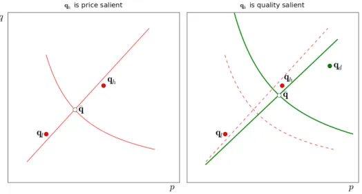
price space, including in regions where it either dominates or is dominated by the reference good q = (q,−p). The resulting salience rankings are graphically represented in Figure 1 below. Note that there is a trade-off between goodqk and the reference goodqin quadrants
Figure 1: Salience of attributes ofqk= (q,−p) depends on its location relative toq= (q,−p).
I (qk < q¯, pk < p¯) and II (qk > q¯, pk > p¯), whereas qk dominates q in quadrant IV and is
dominated by q in quadrantIII.
From the previous discussion, in quadrants I and II the salience ranking of a good is determined by its location relative to the upward sloping curve q/p= ¯q/p¯, along which the good’s quality/price ratio is equal to that of the reference good. This determines, together with the downward sloping curveq·p= ¯q·p¯in the quadrants III and IV, four regions where either price or quality is salient.12 To jointly characterize the salience ranking of all goods in an evoked setCev we simply need to compute the reference quality and price, and then place
the goods in the “windmill” diagram of Figure 1 above. In this diagram, a good’s pricepk is
salient in regions where it is far from the reference price ¯p. Accordingly, the good’s quality
qk is salient in the regions where it is far from the reference quality q. Figure 1 allows us to
limai→0σ(qik, ai). Moreover, when comparingσ(qik,0) andσ(qjk,0), we assume the limit then keeps the ratio
of hedonic utilitiesai/aj constant at 1. Homogeneity of degree zero is stronger than diminishing sensitivity,
as is exemplified by the salience function σ(x, y) = x|+x−y+y|ζ, withζ >0. In this caseσ(αx, αy)> σ(x, y) for
α >1. Thus homogeneity excludes certain weak forms of diminishing sensitivity. 12To identify the downward sloping curve, note that when q
k dominates the reference (i.e. qk > q and
pk < p), thenqk is salient if and only ifσ(qk/q,1)> σ(1, p/pk), namely if and only ifqkpk > qp. Instead,
develop visual intuitions for the role of salience in explaining choices.
2.2
Discussion of Setup and Assumptions
Our model of context-dependent evaluation hinges on two basic facts about perception: i) our perceptive apparatus is structured to detect changes in stimuli (captured by the ordering property), and ii) changes are better detected when they occur close to a baseline reference level (captured by the diminishing sensitivity property). BGS (2012) provide a fuller description of these psychological phenomena. In this paper, we show how the same assumptions shed light on a wide variety of choice patterns and puzzles in a riskless setting. The general approach we follow is also consistent with recent results in neuroeconomics. Hare, Camerer, Rangel (2009) and Fehr and Rangel (2011) provide evidence that subjects evaluate goods by aggregating information about different attributes, with decision weights modulated by attention. In particular, exogenously varying the attention received by differ-ent attributes (e.g., by instructing subjects to attend to the “healthiness” of a snack) results in both higher brain activity associated with the attribute’s decision value, and a higher likelihood that subjects choose the good superior along that attribute. Methodologies from neuroeconomics may be useful to empirically test our model, which makes predictions re-garding not only choice but also attention and valuation.
Our model makes predictions that can be tested both in the lab and in the field. Exper-imental tests are more straightforward because the evoked set would typically coincide with the choice set. Such tests are relatively easier when (as is standard in the experimental lit-erature) the quality dimensions are objective characteristics of a good, such as a car’s speed, mileage, or price. However, our model also applies to cases where the quality of a good is defined by consumer utility, e.g. wine. In this case, the assumption of homogeneity of degree zero of salience (A.0) allows for a straightforward measurement of quality attributes as the subject’s willingness to pay for it.13
In the field, we do not directly observe the evoked set, but a plausible assumption in
13As we show formally in Section 3.4, when stating his willingness to pay WTP for quality q
k in an
experimental setting, the subject evaluates the good (qk,−W T P) in comparison to not having the good,
(0,0). Homogeneity of degree zero then implies that W T P =qk. This argument holds more generally as
many circumstances is that it is populated by the true distribution of future prices, as in the rational expectations model. If one makes additional (and testable) assumptions on price distributions over time, such as that prices follow a random walk, one can define the evoked set precisely, and characterize the effects of salience in terms of surprises relative to expectations. For example, large price increases compared to expectations would make prices more salient. We discuss this issue in more detail in section 4.14
The assumption of homogeneity of degree zero merits further comment. The key predic-tions of our model are shaped by diminishing sensitivity and ordering. For instance, ordering implies that increasing the price of a good increases the salience of its price, provided that price is above average, while diminishing sensitivity implies that price differences become less salient as the level of prices increases. These predictions hold for any increasing utility function, and can be tested experimentally. However, when ordering and diminishing sensi-tivity are in conflict, as when both price levels and price dispersion increase, homogeneity of degree zero pins down the relative importance of each force. It does so in a way closely related to Weber’s law: the salience of an attribute for a good remains constant when the level of that attribute increases in all goods, provided the difference between the good’s level and the reference level increases proportionally. While we do not claim that this assumption is universally applicable, it is supported by an emerging paradigm in psychology stressing that people possess an innate “core number system” which compares magnitudes in terms of ratios.15 Homogeneity of degree zero is thus a plausible assumption, and it allows for precise
predictions on the effect of context on the consumer’s choices, such as the role of the quality to price ratio. These predictions, however, do depend on the consumer’s utility function (in contrast to those of ordering and diminishing sensitivity).
We have also assumed that evaluation depends on the attributes’ salience ranking. This
14It is useful to clarify the difference between a rational expectations formulation of the evoked set and the Koszegi-Rabin (2006) rational expectations approach to reference point determination. Koszegi and Rabin define the reference point to be the agent ˜Os expected consumption path. As a result, the reference point and actual consumption are jointly determined in equilibrium. In our model, the reference point depends on the choice set that the agent expects to face in the future, which is an exogenously given datum.
15Feigenson, Dehaene and Spelke (2004): “To sum up, the findings indicate that infants, children and adults share a common system for quantification.” This system exhibits a logarithmic (i.e. ratio based) representation of numerical magnitude: “numerical representations therefore show two hallmarks: they are ratio-dependent and are robust across multiple modalities of input.” Interestingly, the “system becomes integrated with the symbolic number system used by children and adults for enumeration and computation.”
rank-based discounting aids tractability, but has some shortcomings: i) evaluation is discon-tinuous at those attribute values where salience ranking changes, and ii) evaluation may be non-monotonic. In Appendix A.2 we show that with a continuous salience weighting these shortcomings disappear under general conditions. In the main text, we however stick to the more tractable rank-based discounting. All our results qualitatively carry through with continuous salience.16
Several authors have recently proposed models that endogenize the set of options that come to the decision maker’s mind, as distinct from the choice set (Eliaz and Spiegler 2010, Masatlioglu et al. 2010, Manzini and Mariotti 2010). These models focus on the “consider-ation set” as it is understood in the marketing literature, namely a typically small subset of all available options that the agent actually considers when making a choice.17 In contrast, in the examples and applications in this paper, the choice set is small and the evoked set includes other options that are not in effect available.
Several models of consumer choice incorporate loss aversion relative to a reference good, including Tversky and Kahneman (1991), Tversky and Simonson (1992) and Bodner and Pr-elec (1994). A main implication of these models is a bias towards middle-of-the-road options, which avoid large perceived losses in every attribute. This prediction is hard to reconcile with evidence that in many situations consumers do choose extreme options. Moreover, these models do not speak to the other puzzles reviewed in the Introduction, such as the Savage car radio problem, context dependent WTP or the Hastings-Shapiro data.
Other related models of context dependent evaluation have recently been proposed. The literature on relative thinking assumes that valuation of a good depends on the “referent” levels of its characteristics (Azar 2007, Cunningham 2011). The fundamental assumption is that the marginal utility of a characteristic decreases with the level of its referent. This
16None of our results depend on valuation discontinuities that arise from discrete weighting. Instead, they depend on the fact that a good is overvalued if and only if its most valuable attributes are relatively more salient than its least valuable attributes (see Appendix A.0 for a formalization). The main features of all our results thus survive with a continuous salience function (including the non-monotonicity of willingness to pay, see Section 3.4).
17The determination of the choice set is also an important input in (rational) discrete choice models: the predictions of these models depend quantitatively on how the set of alternatives is specified. Moreover, allowing for incomplete consumer information (Goeree 2008) suggests an important role for (un)awareness of available choices.
is reminiscent of the diminishing sensitivity property of salience, and in fact Cunningham (2011) reproduces some related patterns of choice, such as the Savage car radio puzzle. By assuming that valuation changes are driven solely by diminishing sensitivity, Cunningham’s approach implies that all goods’ valuations are distorted in the same way. Thus, it does not account for patterns of choice in which ordering plays a role, such as the taste for balance (section 3.4) or the Hastings-Shapiro evidence on gasoline (section 4.1).
Koszegi and Szeidl (2011) build a model that centrally features the idea of ordering: their consumers are essentially local thinkers who focus on and overweigh those attributes in which options differ the most in terms of utility. Koszegi and Szeidl then use their model to shed light on biases in intertemporal choice. By neglecting diminishing sensitivity, the Koszegi-Szeidl model predicts a strong bias towards concentration, namely consumers tend to overvalue options whose advantages are concentrated in a single dimension. This bias seems difficult to reconcile with the evidence on diminishing sensitivity (such as the Savage car radio puzzle), and also with the evident desire of luxury manufacturers to avoid shortcomings in any aspect of their merchandise.
By combining diminishing sensitivity with ordering within the context of an evoked set, our model provides a unified account of several well-known choice patterns and puzzles. It reconciles patterns explored separately by Cunningham (2011) and Koszegi and Szeidl (2011), sheds light on phenomena currently gathered under the banner of mental accounting (such as context dependent willingness to pay), and generates new predictions of interest in economic applications.
3
Salience and Choice
We now examine various implications of our model, motivated by the evidence summarized in the introduction. Section 3.1 considers context effects that occur due to a uniform increase in the level of one attribute (price) across all goods. Section 3.2 investigates context effects that occur when new goods are added to the choice set. Section 3.3 studies a taste for balance in goods having two positive quality attributes. Finally, Section 3.4 applies these results to examine how historical prices affect the local thinker’s willingness to pay for quality.
In Sections 3.1 through 3.3, we focus on context effects arising solely from the composition of the choice set. To that end, we assume that prices are stable in the sense that the historical prices recalled by the consumer to populate the evoked set coincide with the current prices,
phist
k = pk for all goods qk. As a consequence, the reference price is just the average price
of goods in the choice set itself (and similarly for the reference quality). We thus simplify notation by describing the choice setting in terms of the choice set alone. In Section 3.4 we explicitly keep track of historical prices and the evoked set.
3.1
Buying Wine in a Store vs. at a Restaurant
In the wine store, the available wines are:
Cstore= qh = (30,−$20) ql = (20,−$10) . (12)
The rational consumer is indifferent between qh and ql because u(qh) = 30 − 20 =
u(ql) = 20−10. This is not true for the local thinker. Since the quality/price ratio of the
low end wine is higher than that of the high end wine (i.e. 20/10> 30/20), Proposition 1 implies that price is salient for both wines. It follows from (10) that the high end wine is undervalued relative to the low end wine, so the local thinker strictly prefers ql to qh. In
the wine store, price is more salient than quality, so the local thinker is overly sensitive to price differences. He perceives ql to be slightly less good, but a lot cheaper than qh.
Suppose now that the same two wines are offered at a restaurant, with uniformly higher prices: Crestaurant= qh = (30,−$60) ql = (20,−$50) . (13)
The rational consumer is again indifferent between qh and ql, because u(qh) = 30−60 =
u(qh) = 20−50. Unlike in the store, however, qh now provides a better quality to price ratio
than ql, since 30/60>20/50. As a consequence, in the restaurant the consumer focuses on
quality and, from (11), the high end wine is chosen over the alternative. At the restaurant the local thinker is less sensitive to price differences and perceives qh to be slightly more
expensive but significantly better than ql. This occurs even though the quality gradient
qh−ql and the price gradient ph−pl are the same in the store and at the restaurant, so that
the rational consumer does not systematically change his choice between the two contexts. Context influences decisions here because the ranking of the quality to price ratio changes from the store to the restaurant. The store displays a higher percentage variation along the price dimension than along the quality dimension, which implies that the cheaper good is the better deal. The reverse is true at the restaurant.
These effects, arising from the diminishing sensitivity of the salience function, naturally deliver a well known feature of consumer behavior: lower price sensitivity for choice among more expensive goods. An example of this phenomenon is Savage’s (1954) car radio prob-lem18, in which a consumer is more likely to buy a car radio when the price of the radio is added to the price of the car than when the radio is sold in isolation, after the car purchase. To see this, denote byq the car’s quality and byq+qr its quality when the radio is installed.
Denote by pthe car’s price and by pr the price of the radio. When choosing whether to buy
the car alone or with the radio, the consumer faces Cbundle ≡ {(q, p),(q+qr, p+pr)}. The
salience of quality for the car with the radio is σ(q+qr, q+qr/2), the salience of its price
is σ(p+pr, p+pr/2). When instead the consumer chooses whether to keep his car without
the radio or to install a radio in it, he faces Cisol ≡ {(q,0),(q+qr, pr)}. The salience of
quality for the car with the radio is still σ(q +qr, q+qr/2) while the salience of its price
is σ(pr, pr/2). By diminishing sensitivity σ(p+pr, p+pr/2) < σ(pr, pr/2), so the price of
the radio is more salient when the radio is bought in isolation. It is easy to check that this analysis is confirmed by the q/p logic under assumption A0.
Similarly, our model sheds light on the jacket and calculator problem (Kahneman and Tversky 1984), in which subjects who have decided to buy a bundle ((jacket,$125),(calculator,$15)) are willing to travel 10 minutes to save $5 when the discount applies to the calculator, but not to the more expensive jacket. Intuitively, walking for 10 minutes (vs. not walking at all) has salience σ(10,5). Saving 5 dollars on the jacket has salience σ(120,122.5); saving them on the calculator has salience σ(10,12.5). Since σ(10,12.5) > σ(120,122.5), the discount is
18This problem was proposed as a counterpart to Allais’ paradox to illustrate the breakdown of the sure thing principle in riskless choice. Salience accounts for both versions of the problem, see BGS (2012).
more likely to be salient if it is applied to the calculator.
These results generalize to choice among an arbitrary number of goods. To see this, suppose that the local thinker is choosing between N > 1 goods located along a rational indifference curve. The indifference condition allows us to identify the effect of salience, abstracting from rational utility differences. Given the quasilinear utility in (1), the N
goods display a constant quality/price gradient, formally qk−qk0 = pk −pk0 for all k, k0 =
1, ..., N. Assume, without loss of generality, that quality and price increase in the index k
(i.e. q1 < ... < qN and p1 < ... < pN). In Appendix A.1 we prove:
Proposition 2 Along a rational linear indifference curve, the local thinker chooses the good with the highest quality/price ratio. In particular:
1) if q1/p1 >1, the cheapest good (q1, p1) has the highest q/p ratio and is chosen;
2) if q1/p1 <1, the most expensive good (qN, pN) has the highest q/p ratio and is chosen;
3) ifq1/p1 = 1, the q/p ratio is constant and the consumer is indifferent between the goods.
Salience tilts the rational linear indifference curves, favoring either the cheapest or the highest quality good. Diminishing sensitivity determines which good is chosen. When, as in case 1), the price level is low relative to the quality level, variation along the price dimenson is more salient than that along the quality dimension. As a consequence, the consumer focuses on prices, breaking indifference in favour of the cheapest good. When, as in case 2), the price level is high relative to the quality level, the consumer attends more to quality differences. As a result, he breaks indifference in favour of the highest quality good. In both cases the consumer prefers the good with the highest quality to price ratio, which is either the cheapest or the highest quality good in the choice set.19
This mechanism differs substantially from models of context dependence based on loss aversion. These models share the broad implication that consumers choose the good which minimizes losses across all attributes (while differing on how precisely such losses are mea-sured). Consider for concreteness Bodner and Prelec’s (1994) model, where consumers eval-uate each good’s gains and losses relative to the same reference good, namely the “centroid”
19The linearity of rational indifference curves (which is due to the quasi linearity of preferences) is useful to obtain such a sharp characterization. For a concave indifference curve, the reference good will lie below the rational indifference curve itself, and so salience rankings will differ across goods. As we show below, concave evoked sets generate decoy effects.
(or average) good in the choice set. As prices increase uniformly, the gains/losses relative to the reference price stay constant, leaving choice unchanged. In our model, in contrast, as prices increase a given price difference becomes less salient. This mechanism highlights the role of diminishing sensitivity of salience, which is evaluated relative to not experiencing an attribute and not with respect to experiencing its reference level.
To visualize Proposition 2, note that with linear utility a rational indifference curve is a positively sloped line in the (q, p) diagram. If the evoked set consists of a collection of points on an indifference line, then the reference good (q,p) also lies on that line. Exploiting these features, Figure 2 graphically represents cases 1) and 2) of Proposition 2.
Figure 2: All goods on an indifference curve have the same salience ranking.
As in the case of the wine store, in the left panel goods vary more along the price than along the quality dimension: price is salient and consumers choose the cheapest good. The reverse holds in the right panel.20
20The local thinker’s tendency to choose extreme goods in the choice set generalizes to any evoked set C lying on a positively sloped line, even if this line is not a rational indifference curve. Also in this case all goods will have the same salience ranking, and the good taking the most favourable value of the salient attribute will thus be maximally overvalued (even if it is not necessarily chosen).
3.2
Decoy Effects and Violations of IIA
There is ample experimental evidence that manipulation of the choice set alters the preference among existing goods, in violation of independence of irrelevant alternatives (IIA). A well documented anomaly in both marketing and psychology is the so called decoy effect (Huber, Payne and Puto 1983, Tversky and Simonson 1993), in which adding an option dominated by one of two goods boosts the demand for the dominating good. Another well known anomaly is the compromise effect (Simonson, 1989), whereby adding an extreme option to a pairwise choice induces subjects to change their preferences toward the middle of the road, or compromise, option. We now show how our model can account for these phenomena as a result of the impact of the added option on salience.
Consider again the wine example in (12), with a variation in which a third, more expensive and higher quality wine qd is added to the wine list
C0= qh = (30,−$20) ql = (20,−$10) Cdecoy= qd = (30,−$30) qh = (30,−$20) ql = (20,−$10) (14)
Wine qd is dominated by qh, yielding lower utility than the orginal options, u(qd) = 0 <
u(qh) =u(ql) = 10. A rational decision maker is indifferent between qh and ql but prefers
both to qd. The inclusion of qd in the evoked set does not affect his choice.
As shown in Section 3.1, in C0 the local thinker picks the low end wineql because it has
the highest quality/price ratio, so prices are salient. What happens when qd is added to the
list? The new wine delivers the highest quality in the choice set, but is much more expensive than the other wines. In particular, the quality/price ratio of qd, 30/30, is lower than the
quality/price ratio of the high end wine qh, 30/20. Now, by comparison with qd, the high
end wine seems a better deal than in the original choice set C0.
To see the implications for choice, note that in the set Cdecoy, the reference wine is
q = (26.7,−$20). The high end wine qh delivers above reference quality 30 > 26.7 at
the reference price $20. Intuitively, the quality of qh becomes salient. The low end wine
dimension remains salient because ql is a better deal than q, formally 20/10>26.7/20. As
a consequence, after the decoy is added, the low end wine remains price salient but the high end wine becomes quality salient. Under this new salience configuration, the local thinker prefers qh to ql. Our model therefore yields a decoy effect: in pairwise choice the local
thinker prefers ql to qh but he switches to qh when an expensive inferior good qd is added,
thus violating IIA.21The intuition is that when the bad dealq
dis added, qh becomes a good
deal as its quality becomes salient.
This argument does not rely on introducing a decoy qd which is necessarily dominated
by the originally neglected option qh. It relies on the introduction in the choice set of an
option which highlights the quality dimension of qh while not being so attractive that it is
itself chosen. Take two goods ql = (ql, pl), qh = (qh, ph), such that qh is chosen if and only
if its quality is salient. Denoting by ∆u= [qh−ql]−[ph−pl] the rational utility difference
between them, this means
−(1−δ)[ph−pl]≤∆u≤(1−δ)[qh−ql] (15)
This condition says that preference reversals occur provided the rational utility difference between the goods is sufficiently close to zero, be it positive or negative: only in this case can a change in salience affect choice among the two goods. We restrict our attention to decoy options qd such that q ≤ qh and p ≤ ph, where (q, p) is the reference good in the enlarged
choice set {ql,qh,qd}. That is, qh is still perceived as having above average quality and
price. The appendix then proves that, when Equation (15) holds, we have:
Proposition 3
i) If ql
pl
> qh ph
, so that price is salient and ql is chosen from {ql,qh}, then for any qd
satisfying qd pd < qh ph + pl pd h qh ph − qh ph i
, good qh is quality salient in {ql,qh,qd}. Moreover, there
exist options qd satisfying the previous condition and qd> qh, pd> ph such that qh is chosen
from {ql,qh,qd}.
ii) If ql
pl
< qh ph
, so quality is salient and qh is chosen from {ql,qh}, then there exist no
decoy options qd such that pqdd ≤ qpll and qh is price salient in {ql,qh,qd}. In particular, for
21Asq
no qd satisfying these properties is ql chosen from {ql,qh,qd}.
Consider first case i). Hereql is a good deal when compared to qh, namelyql/pl> qh/pl
(so that the price dimension is salient) and the consumer prefers ql over qh in a pairwise
choice. Then Proposition 3 says a decoy qd is sufficient to reverse this preference when qd
has a low enough quality-price ratio, namely qd pd < qh ph + pl pd h qh ph − qh ph i
. The decoy must be a “bad deal” in the sense that it lowers the reference quality-price ratio to the point that
qh/ph > q/p. Since the reference quality is now low relative to the reference price, this makes
the quality of qh salient.
The middle good qh is then chosen as long as the decoy itself is not too attractive. This
implies that the decoy effect is strongest when the new optionqdis dominated byqh, with the
same or lower quality but a much higher price [e.g. see example (14)]. However, preference reversals can also occur when the added option qd is not dominated by qh, including when
qd> qh and pd> ph. In this case,qh is perceived as providing intermediate levels of quality
and price. As long asqdprovides a relatively larger increase in price than in quality compared
to qh, the consumer focuses on the quality of qh and is more likely to choose it. This case
provides a rationale for the compromise effect, which in our model arises due to a similar mechanism as the decoy effect.
Figure 3 provides a graphical intuition for the decoy/compromise effect of casei). When the new good qd has a sufficiently lower q/p ratio than existing options, the evoked set
becomes concave with respect to prices. As a result, qh has both higher quality and higher
quality/price ratios than the reference good, becoming quality salient.22
Consider now caseii) of Proposition 3. Nowqh’s quality is already salient in the pairwise
comparison withql. Adding a decoy to the lower quality goodql, namely a bad dealqdwith
relatively low quality to price ratio (as implied by the conditionqd/pd< ql/pl), has no effect
on qh’s salience ranking: in fact, qh remains a high quality, high quality-price ratio good,
so its quality remains salient. A striking implication is that in this case there is no decoy option that boosts the relative evaluation of the lower quality goodql, even for decoys such
that ql is a dominating option (qd < ql, pd > pl).
22In typical illustrations of the compromise effect, the three goods lie on a straight line in attribute space, with the intermediate good equidistant from the other two (Tversky and Simonson, 1993). If utility is concave, this arrangement translates into a concave choice set as in Figure 3.
Figure 3: Adding a decoy changes the quality/price ratio of the reference good. There are instances, not contemplated in Proposition 3, in which a decoy might increase the relative evaluation of a lower quality good.23 However, Proposition 3 captures an
impor-tant asymmetry generated by our model, whereby goods with high quality and high price are more likely to benefit from decoy effects than their low quality, low price competitors. This effect is different from loss aversion (Tversky and Simonson 1993, Bodner and Prelec 1994) in that consumers do not mechanically prefer middle-of-the-road options. It is, however, consis-tent with Heath and Chatterjee (1995)’s survey of experimental results on decoy effects. The authors find that adding appropriate decoys typically boosts experimental subjects’ demand for high quality goods, but rarely for low quality goods.
3.3
Goods with Multiple Positive Quality Attributes
Having examined the tradeoff between quality and price, we now consider the trade-off between two quality dimensions. Several experiments document subjects’ tendency to select options that offer a more balanced combination of positive qualities in the choice set, in accordance with the compromise effect. We now show that this taste for balance arises naturally in our model due to diminishing sensitivity: for unbalanced goods, the salient
attributes are their shortcomings rather than their strengths. This mechanism is richer than loss aversion accounts and yields novel predictions.
Consider goods qk ≡ (q1k, q2k, p) that differ in their qualities but not in their prices, so
that price is the least salient dimension. We omit the price for notational convenience. In this setup, Definition 1 implies that q1k is more salient than q2k for good qk if and only if
σ(q1k, q1)> σ(q2k, q2). Once more, the salience ranking of a good in quality-quality space is
determined by its location relative to the referenceq= (¯q1,q¯2). Goodqkpresents a trade-off
relative to q whenever it has a higher level of one quality but a lower level of the other, namely it lies in quadrants III and IV of the left panel of Figure 1.
Suppose that q1k >q¯1 and q2k <q¯2. Then, homogeneity of degree zero implies that the
upside q1k of good k is salient whenever σ(q1k/q1,1)> σ(1, q2/q2k), which is equivalent to:
q1k·q2k >q¯1·q¯2.
The salience ranking is determined by the quality-quality productq1k·q2k.24 In this respect, a
version of Proposition 1 carries through: if a good is neither dominated by nor dominates the reference good, its relative advantage is salient if and only if it has a higher quality-quality product than the reference good.
Consider now how salience affects choice along a rational indifference curve. In a quality-quality trade-off, rational indifference curves are downward sloping. Unbalanced goods, which increase the level of one attribute at the cost of weakening the other, have low values ofq1·q2. Balanced goods, whose strengths and weaknesses are comparable, have high values
of q1·q2. We then show:
Proposition 4 Let all goods in the choice set be located on a rational indifference curve, with reference goodq= (q1, q2). The consumer chooses the goodqk which is furthest from q,
i.e. maximizes |q1k−q1|, conditional on being more balanced than q, i.e. q1k·q2k > q1·q2. If
all goods are less balanced thanq, the local thinker chooses the most balanced goodqk, which
maximizes q1k·q2k.
24This condition can be directly mapped into our previous analysis of the quality-price tradeoff by noting that one can write the product q1k·q2k as a quality-cost ratioq1k/q−2k1, which measures the added value of
The local thinker picks the good that is most specialized (has the most extreme strength) relative to the reference good, provided that good’s weakness is not so bad that it is noticed. This choice trades off two forces. On the one hand, keeping the salience ranking fixed, the local thinker tries to maximize the salient quality along the rational indifference curve. If the good is more balanced than the reference, its salient quality is its advantage relative to the reference. The local thinker chooses the good which maximizes this advantage, which is measured by the distance |q1k−q1| = |q2k−q2| from the reference. On the other hand,
as the good’s strength becomes more pronounced at the expense of its weakness, the latter becomes increasingly salient due to diminishing sensitivity.25
Let us go back to the quality-price setting of Proposition 3. In that case also, it is diminishing sensitivity that generates the decoy/compromise effect. There, very unbalanced goods are those with high quality and high price. If the choice set is concave with respect to prices, then diminishing sensitivity is very strong for extreme goods, ensuring that their prices are salient. This renders intermediate goods relatively more attractive.
This effect is again different from loss aversion (Tversky and Simonson 1993, Bodner and Prelec 1994) in that consumers do not mechanically prefer middle-of-the-road options. They instead prefer goods that are somewhat specialized in favor of their salient upsides. Unlike in Koszegi and Szeidl’s “bias towards concentration”, specialization here cannot be excessive, because a severe lack of quality in any dimension is highly salient. An uncommonly spacious back seat may enhance consumers’ valuation of a car, but not if this comes at the cost of an extremely small trunk. Producers often specialize a little, rarely a lot.
3.4
Salience and Willingness to Pay
The Willingness to pay (WTP) for quality q is defined as the maximum price at which the consumer is willing to buy q instead of sticking to the outside option of no consumption
q0 = (q0, p0), where typically q0 =p0 = 0. In standard theory, knowledge of q and of q0 are
25Thus, in quality-quality tradeoffs the local thinker does not go all the way to the extreme good, as he does in quality-price trade-offs. In fact, along a quality-price indifference curve, an increase in quality is matched by an increase in price, so that diminishing sensitivity causes both attributes to become less salient. In contrast, along a quality-quality indifference curve one quality increases at the expense of the other. Due to diminishing sensitivity, the reduction in one quality dimension exerts a stronger effect on salience than the increase in the other quality dimension.
sufficient to determine WTP forq (assuming quasi-linear utility).
In contrast to this prediction, evidence suggests that the willingness to pay for a good can be influenced by contextual factors. In a famous experiment (Thaler 1985), subjects were first asked to imagine sunbathing on a beach on a very hot summer day and then to state their willingness to pay for a beer to be bought nearby and brought to them by a friend. Subjects stated a higher willingness to pay when the place from which a beer is bought was specified to be a nearby resort hotel than when it was a nearby grocery store. Thus, the source of beer influences the subject’s willingness to pay even though the consumption experience is identical in the two scenarios (back at the beach).
Thaler’s explanation for this effect is based on “mental accounting.” First, information about the nearby location prompts the subject to imagine a price for the beer, such as a price experienced in the past at a similar location. This evoked price forms a mental account, which the subject uses to assess his WTP. Second, and crucially, the consumer is assumed to derive a distinct transaction utility from buying a good below its evoked price. Because at the resort the evoked price is higher, the transaction utility associated with buying there at a given price is also higher, so the consumer states a higher WTP for beer from the resort.
In our model, the nearby location also prompts the decision maker to imagine a price for beer, which is included in the evoked set. However, our explanation does not rely on transaction utility. Instead, the recalled price affects salience. When thinking of the high price at the resort, the local thinker is willing to pay a high price for the beer and still perceive quality as salient. When thinking of the low price in the store, however, the local thinker is not willing to pay a high price for the beer, as that price would be very salient. The recalled price acts as an anchor for the consumer, through its effect on salience.
To see this formally, suppose that the consumer must state his WTP for quality q while recalling one historical price ˆp at which the same quality was sold in the past, namely a good ˆq = (q,−pˆ).26 Since the consumer is evaluating the good q = (q,−p) for a price p,
his evoked set is Cev ≡ {q0,ˆq,q}, where the good q0 = (0,0) is the outside option of not
26Alternatively, context might induce the consumer to recall an entire distributionq1, . . . ,q
N of historical
prices. In the beer example, the consumer might recall several past resort or store prices for beer of quality
consuming q. We define the consumer’s willingness to pay for q in the context of ˆq as:
WTP(q|ˆq) = supp (16)
s.t. uLT(q|Cev)≥uLT(q0|Cev).
WTP is still defined as the maximum price p that the consumer is willing to pay for q
against the prospect of obtaining the outside option q0 = (0,0), but the superscript LT
indicates that now the consumer’s preferences are distorted by salience. This change has one crucial implication: different values ofp can alter the salience ofq, changing the consumer’s valuation of the good. As a consequence, the maximization in (16) tends to select a price p
such that q is salient.
In the evoked set Cev, the reference good has quality q = q· 32 and price p = p+ ˆ3p. We
can then show:
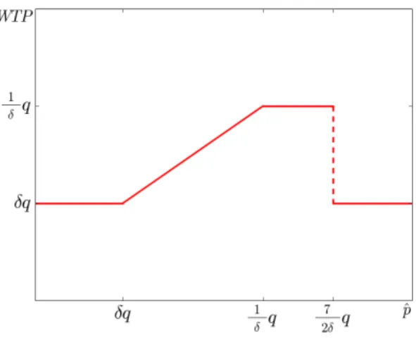
Proposition 5 The consumer’s willingness to pay for q depends on the price pˆas follows:
W T P(q|C) = δq if pb≤δq b p if δq <pb≤ 1 δ ·q q/δ if 1δ ·q <pb≤ 7 2δ ·q δq if bp > 27δ ·q (17)
As δ →1, the willingness to pay tends to q and becomes independent of context pb.
The price context pbonly affects WTP if the consumer is a local thinker, i.e. if δ < 1. If δ = 1, Equation (16) converges to the standard case where WTP equals q and does not depend on pb.
For pb ≤ 7
2δq the consumer’s WTP weakly increases in the average price of alternative
goods bp. In contexts where quality is more expensive, namely pbis higher, the consumer is willing to pay a higher pricep and still view quality as salient.27 The highest possible WTP
isq/δ, which is the consumer’s valuation when quality is salient. Through salience, a higher price pbacts like an anchor, increasing WTP.
27Put differently, as b
Interestingly, Proposition 5 suggests that when the reference price is implausibly high, this effect vanishes. Since for any evaluation of quality q the salience of quality is fixed, if pb
is too high (ˆp >> q/δ) price becomes salient and the consumer’s WTP drops. The WTP in (16) is graphically represented in Figure 4.
Figure 4: Willingness to Pay for q as a function of reference pricep1.
To see how Thaler’s example works in our model, imagine that - upon learning that the nearby location is a resort - subjects populate their evoked set by recalling beer prices that they experienced (or expect) in resorts, denoted ˆpresort. The reference price for the store is
ˆ
pstore. Naturally, ˆpresort >pˆstore. The model says that, provided the reference prices do not
preclude all trade (i.e. bpresort,pbstore < q/δ), the consumer’s WTP is weakly higher at the
resort than in the store, consistent with Thaler’s example.
This analysis shows that in our model context shapes evaluation not only through the characteristics of the alternatives of choice, as in Sections 3.1 and 3.2, but also through the reference options that enter the consumer’s evoked set. Take for example the choice of wine in a store versus at a restaurant. Although as we showed in Section 3.1 the higher prices at the restaurant induce the consumer to select high quality wines, this is unlikely to happen if wine prices are outrageous even by restaurant standards. Unexpectedly high wine prices at a restaurant will be very salient to the consumer, even if price differences among the actual options of choice are fairly small. In other words, salience is not only shaped by the actual options in the choice set, but also by the extent to which the options of choice differ from