WP 05-09
Carlos Llano
Universidad Autonoma de Madrid, Spain
Wolfgang Polasek
Institute for Advanced Studies, Vienna, Austria
and The Rimini Centre for Economic Analysis, Italy
Richard Sellner
Institute for Advanced Studies, Vienna, Austria
B
AYESIAN
M
ETHODS
FOR
C
OMPLETING
D
ATA
IN
S
PACE
-T
IME
P
ANEL
M
ODELS
Copyright belongs to the author. Small sections of the text, not exceeding three paragraphs, can be used
provided proper acknowledgement is given.
The
Rimini Centre for Economic Analysis
(RCEA) was established in March 2007. RCEA is a private,
non-profit organization dedicated to independent research in Applied and Theoretical Economics and related
fields. RCEA organizes seminars and workshops, sponsors a general interest journal
The Review of
Economic Analysis
,
and organizes a biennial conference:
Small Open Economies in the Globalized World
(SOEGW). Scientific work contributed by the RCEA Scholars is published in the RCEA Working Papers
series
.
The views expressed in this paper are those of the authors. No responsibility for them should be attributed to
the Rimini Centre for Economic Analysis
.
The Rimini Centre for Economic Analysis
Bayesian methods for completing data in space-time
panel models
ICarlos Llano∗,a, Wolfgang Polasekb, Richard Sellnerb
aUniversidad Aut´onoma de Madrid, Facultad de Ciencias Econ´omicas y Empresariales,
Departamento de An´alisis Econ´omico, 28049 Madrid
bInstitute for Advanced Studies, Stumpergasse 56, 1060 Vienna, Austria
Abstract
Completing data sets that are collected in heterogeneous units is a quite frequent problem. Chow and Lin (1971) were the first to develop a unified framework for the three problems (interpolation, extrapolation and distribution) of predicting times series by related series (the ‘indicators’). This paper develops a spatial Chow-Lin procedure for cross-sectional and panel data and compares the classi-cal and Bayesian estimation methods. We outline the error covariance structure in a spatial context and derive the BLUE for the ML and Bayesian MCMC esti-mation. Finally, we apply the procedure to Spanish regional GDP data between 2000-2004. We assume that only NUTS-2 GDP is known and predict GDP at NUTS-3 level by using socio-economic and spatial information available at NUTS-3. The spatial neighborhood is defined by either km distance, travel time, contiguity and trade relationships. After running some sensitivity analysis, we present the forecast accuracy criteria comparing the predicted values with the observed ones.
Key words: Interpolation, Spatial panel econometrics, MCMC, Spatial
IThis article has been developed in the context of a research project funded by the Spanish
Ministry of Education and Science within the ’Programa de Movilidad’, REF: SAB2006-0026,between January 2008 and March 2008.
∗Corresponding author: Universidad Aut´onoma de Madrid, Facultad de Ciencias
Econ´omicas y Empresariales, Departamento de An´alisis Econ´omico, 28049 Madrid. Phone: +34 914972910, Fax: +34 914977069.
Chow-Lin, missing regional data, Spanish provinces, ’polycentric-periphery’ relationship.
JEL:C11, C15, C52, E17, R12
1. Introduction
The use of regional (i.e. sub-national) statistics for econometric models is increasingly important for European politics. However, even in the most de-veloped statistics systems, important data restrictions arise when the aim is to obtain regional data at a lower temporal or spatial level. From a tempo-ral perspective, since the 1960’s we are confronted with the unavailability of appropriate short-term indicators (published on monthly or quarterly basis) at the regional level. This limitation restricts the possibility of an accurate follow-up of the regional economy, where an increasing share of the public budget is being managed. With the aim of overcoming this first limitation, different interpolation methods have been developed, for example, with the the aim of estimating quarterly regional accounts (e.g. OECD, 1996; Pavia-Miralles and Cabrer-Borras, 2007), using both univariate (e.g. Boot et al., 1967; Denton, 1971; Friedman, 1962; Chow and Lin, 1971; Fernandez, 1981; Litterman, 1983) and multivariate approaches (e.g. Rossi, 1982; Di Fonzo, 1990). On the other hand, from the territorial view point, it is difficult to find coherent databases covering even the most basic indicators for sub-national units at different spatial disaggregation levels (regional, provincial, local or point data). The consequence are obvious when one takes into account the heterogeneity of space and the effect of different administrative borders in the spatial concentration of the economic activity. Several examples could illustrate the importance of this issue. First, some recent papers in the field of the New Economic Geography point out that the aggregation bias affecting the measurement of economies of agglomeration
stems from the type of spatial units usually considered in the data (e.g. Duran-ton and Overman, 2005, 2008). Another illustrative example can be found in the studies of regional integration and trade (e.g. Helliwell and Verdier, 2000; Hillberry, 2002; Poncet, 2003, 2005), where the unavailability of rich databases covering different spatial levels impede the right evaluation of the integration processes occurring within a country or a group of countries. The relevance of this issue is clear in the case of the European Union, where a lot of effort is being put in the reduction of regional inequalities through the regional and cohesion policy of the EU. The evaluation of this policy, which accounts for the largest part of the EU expenses, is critically affected by the availability of good regional statistics needed for the assignment and surveillance of the EU Funds. With this aim (among others), during more than a decade, Eurostat publishes regional data on a range of different statistical topics, collected by the 27 mem-ber states, but also from the three candidate countries and from the four EFTA states. Usually, this information is collected at different spatial levels based on the nomenclature of territorial units for statistics (NUTS).
NUTS data are collected by the individual member states using common rules and methods. However, not all member states have developed the same level and speed of skills, especially after 1995 when the harmonized European economic account system started. This leads to inhomogeneous data quality and sometimes to holes in the data base, especially of it comes to smaller regional units. Thus, although in 2003 the NUTS system was acquired as a legal basis, and is enjoined on any new member country, it is common to find that the data at the lowest levels of disaggregation (NUTS-3) is missing for some countries and indicators. Moreover, periodical changes in the NUTS regulation occur since the regional classification adapts to the new administrative boundaries or economic circumstances. Consequently, these changes leads to additional
dis-connections in the time series, which can lead to breaks in the information at the lowest spatial units under consideration. Therefore, sometimes it is difficult to obtain stable panel data of all EU regions at the NUTS-3 level covering even the most basic indicators referred to demographics, labor markets, infrastructure, prices or productivity. For example, if one downloads the Eurostat information for regional GDP at the NUTS-3 level for the EU 27, including EFTA and the candidate countries for the period 1995-2005, one would find that 15% of the figures are missing. On the top of that, the problems of data restriction at the NUTS-3 level increases for more disaggregated components of the regional accounts, either from the supply (Gross Value Added by industries), the de-mand (investments, public or public expenses) or the income side (salaries or capital remuneration). Finally, as it has been described above, it could also be the case that the right spatial level for analyzing a specific economic phe-nomenon requires the use of data even at a lower level of aggregation as the NUTS-3. All these facts emphasize the importance of developing spatial inter-polation methods. Besides the temporal limitation of the data, the problem of spatial interpolation of sub-national variables has received minor attention by the official statistics systems. Furthermore, the academic literature available on this topic is less compact and rooted in the main stream of economic statistics. Although there is an abundant literature dealing with the problem of spatial interpolation (from point data to area and vice versa) of physical phenomena and environmental issues (e.g. Kyriakidis and Yoo, 2005; Yoo and Kyriakidis, 2006; Huerta et al., 2004; Guttorp et al., 1994), the number of references de-creases when we focus on the interpolation of economic data at the sub-national level. Among the exceptions, LeSage and Pace (2004) use spatial econometric techniques to estimate missing dependent data. They predict unobserved house prices by using the information of sold and unsold houses to increase the
estima-tion efficiency. LeSage and Pace (2004) predict unobserved spatially dependent data with observable at the same regional level. Our approach is more related to the classical temporal Chow-Lin procedure, but where we now observe the indicators at the disaggregated regional level and need to predict unobserved dependent variables at the same region.
In this paper we suggest two extensions of theChow and Lin (1971) method, the workhorse of the current literature on temporal interpolation: First, we will apply the procedure to regional cross-sectional data using a spatial econometrics model (see Anselin, 1988) and second we will embed the model into a Bayesian framework. We address the problem of a regional data set that is completely observed at an aggregate level (like NUTS-2) and has to be broken down into smaller regional units (e.g. NUTS-3) conditional on observable indicators. We propose a spatial econometrics model in a classical or Bayesian framework, the latter one has to be estimated by MCMC. These methods are developed both for cross-sectional and panel data.
The paper is organized as follows. Section 2 outlines the Maximum Likeli-hood (ML) model of the spatial Chow-Lin (CL) method for cross-sectional data. The classical (BLUE) estimator for the spatial autoregressive model (SAR) is derived, along with the error covariance matrix needed for the improved pre-diction of the missing values, which leads to the so-called spatial gain terms for predictions. In section 3 we extend the approach to a spatial panel model assuming a seemingly unrelated type of covariance structure. The next two sec-tions (4 and 5) consider Bayesian approaches for the spatial Chow-Lin method for cross-sectional and panel data. In these sections the MCMC algorithms and predictions densities are formalized. Applied examples for the procedures are given in section 6. We apply the spatial cross-sectional and panel Chow-Lin method to Spanish NUTS-2 and NUTS-3 data. As we observe all data on the
disaggregated level, we will evaluate the quality of the spatial Chow-Lin method by comparing the predicted values for the NUTS-3 GDP to their observed values and calculate the usual forecast accuracy criteria. A final section concludes.
2. The maximum likelihood Chow-Lin method for completing cross-sectional data
2.1. The Chow-Lin Method
High frequency time series data of the economy is a valuable information for policy makers. However, such data on a monthly or quarterly basis are rarely available. In the past a lot of attempts have been made to interpolate missing high frequency data by using related series that are known. Friedman (1962) suggested relating the series in a linear regression framework. The three prob-lems in connection of missing data are known by statisticians as interpolation, extrapolation and the distributional problem of time series by related series. Interpolation is used to generate higher frequency level (or stock) data, while extrapolation extends given series outside the sample period, and in the dis-tribution framwork one allocates lower frequency flow data, such as GDP (see Fernandez, 1981), to higher frequency observations. The path-breaking paper by Chow and Lin (1971) embedded the missing data problem to a predictive sys-tem framework of aggregate and disaggregate data, leading to boost in research on this topic.
Assuming a linear relationship for the high frequency datay=Xβ+, where
yis a (T×1) vector of unobserved high frequency data,X is a (T×k) matrix of observed regressors, β is a (k×1) vector of regression coefficients and is a vector of random disturbances, with meanE() = 0 and covariance matrix
E(0) = σΩ, Chow and Lin (1971) showed that the BLUE for the regression parameter ˆβ and the unobserved high frequency data ˆy is given by:
ˆ
β = (X0C0(CΩC0)−1CX)−1X0C0(CΩC0)−1y (1) ˆ
y = Xβˆ+ ΩC0(CΩC0)−1(y−CXβˆ), (2)
where C is an×N aggregation matrix consisting of 0’s and 1’s, indicating which cells have to be aggregated together. The essential part in the equation 1 and 2 is the residual covariance matrix Ω, which has to be estimated. The Chow-Lin construction of the BLUE requires knowledge or assumptions about this error covariance matrix. In the literature assumptions like random walk, white noise, Markov random walk or autoregressive process of order one have been suggested and tested (e.g. Fernandez, 1981; Di Fonzo, 1990; Litterman, 1983; Pavia-Miralles et al., 2003). Some authors extended the framework for the multivariate case (e.g. Rossi, 1982; Di Fonzo, 1990) covering time and space for example (e.g. Pavia-Miralles and Cabrer-Borras, 2007). Usually, constraints are imposed to restrict the predicted unobserved series to add up to the observed lower frequency series, e.g. by specifying penalty functions (e.g. Denton, 1971). In this case, the discrepancy between the sum of the predicted high frequency observations and the corresponding low frequency observation is divided up over the high frequency data through some assumptions (for examplepro rata).
There are various problems that may arise when applying the Chow-Lin procedure empirically. First, one has to find a suitable set of observable high frequency indicators. Predicted outcomes may heavily rely on the indicators chosen and their statistical properties. Seasonally adjusting the data and ag-gregating multi-collinear variables improves the quality the results (see Pavia-Miralles and Cabrer-Borras, 2007, for Monte Carlo evidence). Another crucial fact is, of course, the design of the residual covariance matrix and the restrictions
2.2. The spatial extension of the classical Chow-Lin method
Consider a cross-sectional model of nregions where we fit a spatial autore-gressive (SAR) model for the disaggregated units
y=ρW y+Xβ+, ∼ N[0, σ2In]. (3)
The reduced form is obtained by the spread matrixR=In−ρW for an
appro-priately chosen weight matrix W:
y=R−1Xβ+R−1, R−1 ∼ N[0, σ2(R0R)−1]. (4)
The aggregation of the reduced form model is obtained by multiplying with the
N×nmatrix C
Cy=CR−1Xβ+CR−1, CR−1 ∼ N[0, σ2C(R0R)−1C0]. (5)
We will write shorter for the covariance matrix:
σ2Σρ=σ2C(R0R)−1C0. (6)
In the Chow-Lin framework, the aggregated model is always observed with complete data. Therefore, we can estimate it by standard maximum likelihood methods, although the estimates can be quite unreliable because only fewer ob-servations are available in an aggregate level. Based on the coefficients estimate of the aggregated model we can forecast the missing values at the disaggregate level. This is possible in two ways: the first way neglects the system frame-work of the Chow-Lin method, i.e. the seemingly unrelated correlation of the aggregated and the disaggregated model and is therefore the usual univariate regression forecasts, in this paper called Chow-Lin without gain. This simple or
’no-gain’ forecasts is given by the point forecast at the observed low-frequency indicatorX (the mean of the conditional model 3):
y=R−1ρˆ Xβ,ˆ (7)
with the estimated spread matrixRρˆ=In−ρWˆ . For the no-gain prediction, all
theXvariables at the disaggregated level have to be known for allnregions. The second method uses the spatial correlation structure between the aggregated and the disaggregated model and we obtain forecasts with the gain, i.e. conditional normal estimates, where we condition the disaggregated forecasts on the known values of the aggregated model. This leads to the formula that is similar to the temporal Chow-Lin method:
ˆ
yj=Xjβˆ+Gˆe, (8)
where theGeˆis the ”gain-in-mean” term and is an improvement of the naive or simple forecast of the missing y-value at j: ˆyj. The gain is the product of
the estimated aggregated error vector ˆe=ya−Xaρβˆand the ’gain matrix’, first
used by Goldberger (1962)
G= Ω−1ρ C0(CΩ−1ρ C0)−1. (9)
Ω is the covariance matrix link between the aggregated and the disaggregated model and the indexajust is a reminder that it is the regressor matrix of the aggregated model. It also depends on the estimated ρ. Note that if ρ = 0 then Ωa,ρ =IT and the gain matrix reduces to a transposed projection matrix:
because CC0 gives a diagonal matrix with the number of subregions for each aggregated region. Thus, the gain component Geˆ is a vector which is in the
ρ= 0 case a down-weighted aggregated residual of the aggregated fit: A large residual will be smoothed out over n subregions and 1/n-th is added to the simple (no-gain) forecasts. For example, if a certain region has a residual that lies below average, then all the disaggregated forecasts with gains will have their simple forecasts corrected downward. The same will happen in the other direction, when the aggregated residual is positive.
The effect of a spatial ρis a ’spatial smearing out’ of these 1/n discounted aggregated residual to the spatial neighbors. Thus, these point forecasts for the disaggregated model are called ’with gain’ in this paper. First the model and estimators are derived and then a feasible estimator for the prediction is constructed. In section 4 we outline the Bayesian extension to the problem.
3. The maximum likelihood Chow-Lin method for completing panel data
In this section we consider a T×N panel matrixY0 = [y1., ..., yt.], where
each rowt can be considered as a spatial cross-sectional model. Thus, for the T time points we assume the same model as in (3):
yt=ρW yt+Xtβ+t, t∼N[0, σ2In]. (10)
The reduced form is obtained by the spread matrixR=In−ρW for an
appro-priately chosen weight matrix W:
withR−1t∼N[0, σ2(R0R)−1]. Since we assume that the regression coefficients
X are independent of time, we can construct a stacked regression system of the
T equations. This is equivalent to vectorizing the (T×N) panel matrixY into one (T N×1) column vector: y=vec(Y). The same can be done for the residual matrix: =vecE. The (T N×K) regressor matrixX need to be stacked:
y= y1 ... yT , X = X1 ... XT ,W˜ =diag(W1, ..., WT).
Then the stacked regression system can be written as the system before in (3):
y=ρW y˜ +Xβ+, ∼N[0, σΩ⊗In]. (12)
The spatial neighborhood matrix now is defined by a Kronecker product, since the neighborhood matrixW is assumed to be constant across time ˜W =
I⊗W1. The Ω : T ×T matrix is the covariance matrix between theT time
points. If we standardize Ω to a correlation matrix then we obtain in the off-diagonal elements the average time correlations across the cross-sections. The reduced form of the stacked system is given by
y= ˜R−1Xβ+ ˜R−1, R˜−1 ∼ N[0, σ2Ω⊗(R0R)−1].
Note that the covariance matrix of the term ˜R−1is given by
σ2Ωρ= ( ˜R0(Ω⊗IN) ˜R)−1= Ω⊗(R0R)−1. (13) 1If the neighborhood matrix can vary with time we can use a block diagonal matrix:
˜
W =diag(W1, ..., WT). The only difference to the above assumptions is that we assume a
since the stacked spread matrix
˜
R=I⊗I−ρI⊗W =I⊗Rρ (14)
with the spread matrix Rρ defined in the usual way Rρ = I−ρW. The
C-aggregated reduced form is obtained by multiplying with theN T ×n matrix ˜
C=IT ⊗C
˜
Cy= ˜CR˜−1Xβ+ ˜CR˜−1, C˜R˜−1 ∼ N[0,Ωρ=σ2Ω⊗Σρ].
Notice that the terms in the aggregated X matrix can be simplified: ˜y = ˜
Cy=vecY C0 or ˜yt=Cyt, sinceC is a (N×N) matrix. and
Xa = ˜CR˜−1X=I⊗CR−1X
which factors for each regressor block intoXa,t=CR−1Xt, t= 1, ..., T.
We find that the covariance matrix of ˜CR˜−1 is given by:
Ωρ= ( ˜R0(Ω⊗IN) ˜R)−1= Ω⊗σ2(R0R)−1= Ω⊗σ2Σρ. (15)
where Σρis given as in (6). Thus, we see that the covariance matrix is just a
Kronecker product between the SUR covariance matrix Ω and the usual spread precision Σρ = (R0R)−1. We can simply adapt the usual SAR algorithms for
a GLS estimation of the stacked spatial panel Chow-Lin model. Note that the covariance matrix can be estimated as ˆΩ =EaEa0/N :T×T withEa =Ya−Yˆa:
T×N and ˆYa= [X1β, ..., Xˆ Nβˆ].
model (3):
yt=R−1ρˆ Xtβ,ˆ t= 1, ..., T. (16)
where Rρˆ is given as before in (14). This is because the ˜R matrix is a block
diagonal matrix.
The conditional Chow-Lin predictions are given by
ˆ
yt=Xtβˆ+Geˆa,t t= 1, ..., T (17)
where theGeˆa,tis an improvement of the estimated aggregated error term ˆea =
(ya−Xaρβˆ) using the ’gain matrix’
Ga = Σ−1ρ C0(CΣρ−1C0)−1=IT ⊗G, (18)
and Σρis the same disaggregated covariance matrix as in the univariate case.
Interestingly, the Σρ matrix cancels out, because of (15) we have Ω−1ρ C0 =
Ω−1⊗(R0R) and reduces Ga = IT ⊗G with the univariateG given in (18).
Thus, Σρ plays no role in the Chow-Lin gain of the spatial panel completion
model. The gain matrix G is constant over time and depends only on the spread matrix R and the aggregation matrix C.
Is there a difference between stacked and simple Chow-Lin forecast? First of all, there is a better statistical basis as more data are used in the estimation process. But surprisingly, the correlation matrix between time points (Ω) seems not to be directly involved in the prediction process. But, as we will see in the next section, the Ω matrix is part in the 2-step estimation process, which is outlined in the next section. Thus, there is an indirect influence of the time correlations in the panel model on the predictions. If this bit of extra information will
improve the forecasts can not be decided on a theoretical basis. We will need forecast criteria and experience if this is the case. Note that in the Bayesian model, the Chow-Lin completion depends on the Ω matrix. In general, a better fit leads to better forecasts. It needs to be seen if this observation is also true for the Chow-Lin case: Bayesian methods and feasible GLS methods usually do not produce betterR2but might smooth out extreme observations that disturb
the link between the aggregated and the disaggregated fit in a spatial Chow-Lin model.
3.1. The 2-step feasible GLS estimator
In the section we show how we can extend the ’mixed SAR’ estimation of LeSage(1999) to incorporate the estimation of the SUR covariance matrix. The 2-step feasible GLS estimator has to be estimated by the following steps:
• OLS estimation in the modely=Xβ0+u0 • OLS estimation in the modelW y=Xβ1+u1
• Compute OLS residualse0=y−Xβˆ0 ande1=y−Xβˆ1 • ρˆ: Maximize the concentrated likelihood function
L(ρ) =ln(1/n)(e0−ρe1)0(e0−ρe1)n/2 +ln|I−ρW˜|
• Compute ˆβ= ˆβ0−ρβˆ1and ˆσ2= (e0−ρe1)0(e0−ρe1)/nT • Compute ˆΩ = ˆE0E/nˆ with ˆe=vec( ˆE) and ˆe=y−ρW yˆ −Xβˆ
• GLS estimation in the modely=Xβ0+u0 with ˆΣ = ˆΩ⊗In • GLS estimation in the modelW y=Xβ1+u1with ˆΣ = ˆΩ⊗In • Compute the GLS residualse0=y−Xβˆ0 ande1=y−Xβˆ1
• ρˆ: Maximize the concentrated likelihood function
L(ρ) =ln(1/n)(e0−ρe1)0(e0−ρe1)n/2 +ln|I−ρW˜|
• Compute ˆβGLS = ˆβ0−ρβˆ1 and ˆσGLS2 = (e0−ρe1)0(e0−ρe1)/nT
Finally the GLS estimates ˆβGLS can be used for Chow-Lin predictions of the
missing low-frequency data.
4. The Bayesian Chow-Lin model for completing cross-sectional data
We consider a cross-sectional spatial autoregressive (SAR) model as in (10)
y=ρW y+Xβ+, ∼N[0, σ2In].
The model assumes that we have a cross-sectional vectory = yt :N ×1 at a
certain point in time t, which is not observed, but we can observe a shorter, aggregated vectorCy:n×1. We consider the disaggregation spatial regression model
y=ρW y+Xβ+, t∼N[0, σ2In]. (19)
The reduced form is obtained by the spread matrix R for an appropriately chosen weight matrix W:R=In−ρW
y=R−1Xβ+R−1, R−1∼N[0, σ2(R0R)−1]. (20)
The prior distribution for the parametersθ= (β, σ−2, ρ) is proportional to
since we assume a uniform prior for ρ ∼ U[−1,1]. The C-aggregation of the reduced form model is obtained by multiplying with theN×nmatrix C
Cyt=CR−1Xβ+CR−1t, CR−1t∼N[0, σ2C(R0R)−1C0]. (21)
We will write shorter for the covariance matrix:
σ2Ωρ=σ2C(R0R)−1C0. (22)
The joint distribution ofθ= (β, ρ, σ2) of this model is given by
p(θ|y) =N[CR−1Xβ, σ2Ωρ]· N[β |β∗, H∗]·Γ(σ−2|s2∗, n∗) (23)
4.1. MCMC for the SAR-CSCL model
Consider the SAR cross-sectional Chow-Lin (SAR-CSCL) model and let us denote the 3 conditional distributions byp(ρ|θc), p(β|θc),andp(σ2|θc) where
θ= (ρ, β, σ2) denotes all the parameter of the model andθcthe complementary parameters in the f.c.d.’s, respectively. The MCMC procedure consists of 3 blocks of sampling, as is shown in the next theorem:
Theorem 1 (MCMC in the SAR-CSCL model). The MCMC es-timation for the SAR-CSCL model involves the following iterations:
Step 1. Drawβ fromN[β | b∗∗,H∗∗]
Step 2. Drawρi by a Metropolis step: ρnew=ρold+N(0, τ2)
Step 3. Drawσ−2 fromΓ[σ−2|s2∗∗n∗∗/2, n∗∗/2]
Step 4. Repeat until convergence.
Proof 1 (Proof of Theorem 1).
(a) The fcd for the beta regression coefficients is
p(β|y, θc) = N[β |b∗, H∗]·N[Cy|CR−1Xβ, σ2C(R0R)−1C0]
with the parameters
H∗∗−1 = H∗−1b∗+σ−2X0R0−1C0Ω−1ρ CR−1X,
b∗∗ = H∗∗[H∗−1b∗+σ−2X0R0−1C0Ω−1ρ Cy]
(b) For the fcd of the residual variance we find
p(σ−2|y, θc) = Γ[σ−2|s2∗∗n∗∗/2, n∗∗/2] (24)
with n∗∗ =n∗+nand s2∗∗n∗∗=s2∗n∗+ESSρ and where the error sum of
squares ESSρ is given by
ESSρ= (Cy−CR−1Xβ)0Ω−1ρ (Cy−CR
−1Xβ). (25)
(c) For the fcd of the spatial ρwe use a Metropolis step:
ρnew=ρold+N(0, τ2) with α=min
1,p(ρnew) p(ρold)
,
the acceptance ratio, and where p(ρ)is the (kernel of ) the full conditional forρ, in our case the kernel is just stemming from the likelihood function:
p(ρ) =|Ωρ|− 1
2exp(− 1
σ2ESSρ), (26)
with ESSρ given in (25).
From the MCMC simulation we obtain a numerical sample of the posterior distributionp(β, ρ, σ−2|y).
4.2. Completing data by prediction
We obtain the posterior predictive distribution in the following way, by in-tegrating over the conditional predictive distribution with the posterior distri-bution
p(yp|y) = Z Z Z
p(yp|β, σ−2)p(β, ρ, σ−2|y)dβdρdσ−2
where the posterior normal-gamma density p(β, ρ, σ−2 | y) is found numeri-cally by the MCMC sample, yielding a posterior sample of theθ parameters:
tive sample of the unknown vectoryby drawing from the reduced form (which depends on the matrix W and on the known regressorsX):
y(j)∼N[R−1j Xβj+gj, σ2j[(Rj0Rj)−1−Gj]], (27)
with Rj = In−ρjW, j = 1, ..., J and g is the gain vector and G is the gain
matrix for the mean and variance matrix, respectively, which are defined by
Gj = (R0jRj)−1C0[C(R0jRj)−1C0]−1C(Rj0Rj)−1], (28)
gj = (R0jRj)−1C0[C(Rj0Rj)−1C0]−1(yagg−yˆagg,j)], (29)
where we use the aggregated residuals ˆeagg=yagg−yˆagg and the current
pre-dictions ˆyagg,j =R−1agg,jXaggβj.
5. The Bayesian Chow-Lin model for completing panel data
We consider a panel spatial autoregressive model as in (10)
yt=ρW yt+Xtβ+t, ∼N[0,Ω⊗σ2In]
with the residuals=vecE from the stacked residual matrixE :T×n . The prior information for the parametersθ= (ρ, β, σ2,Ω) is blockwise independent
p(ρ) =U(−1,1);p(β) =N(β∗, H∗);p(σ−2) = Γ(s2∗, n∗), p(Ω−1) =W(Ω∗, ν∗),
where U is a uniform,W a Wishart and Γ a Gamma-2 distribution. Consider the SAR panel Chow-Lin model (in short SAR-PCL) and let us denote the 3 conditional distributions byp(ρ|θc), p(β |θc),andp(σ2|θc) where θc denotes
The MCMC procedure consists of 4 blocks of sampling, as given in the next theorem:
Theorem 2 (MCMC in the SAR-PCL model).
The MCMC estimation for the SAR-PCL model involves the following iterations:
Step 1. Drawβ fromN[β | b∗∗,H∗∗]
Step 2. Drawρby a Metropolis step: ρnew=ρold+N(0, τ2)
Step 3. Drawσ−2 fromΓ[σ−2|s2 ∗∗, n∗∗]
Step 4. DrawΩ−1 from W[σ−2|Ω∗∗, ν∗∗]
Step 5. Repeat until convergence.
Proof 2 (Proof of Theorem 2). The first 3 fcd’s are the same as in Theorem 1. We now show that the fcd for theΩ−1is derived in the following way. Recall that the reduced form of the panel SAR model is given by
y∼N[R−1Xβ,Ω⊗σ2(R0R)−1]. (30)
This leads to the likelihood function
p(Ω−1|y) =|Ω⊗σ2(R0R)−1|−1/2exp{− 1
2σ2e
0(Ω⊗σ2(R0R)−1)−1e}, (31)
withe=y−R−1Xβ=vec(E)the vectorisation of the residual matrixE:T×n. This leads to the compact form
p(Ω−1|y) =|Ω|−n/2σ−nT|R|exp{− 1
2σ2trEΩE
0(R0R)−1}. (32)
Now this expression has to be combined with the kernel of the prior distribution
p(Ω−1|y)∝ |Ω|−ν∗/2exp{− 1
2σ2trΩ∗Ω}=W(Ω∗∗, ν∗∗). (33)
and yields a Wishart distribution withν∗∗=ν∗+nandΩ∗∗= Ω∗+E0(R0R)−1E.
5.1. Completing data by prediction
We obtain the posterior predictive distribution in the same way as before: Using the above MCMC procedure we obtain a posterior sample of the θ pa-rameters: ΘM CM C ={(βj, ρj, σj2,Ωj), j = 1, ..., J}.Again, from this MCMC
output we find a predictive sampleyby drawing from the reduced form (which depends on the matrix W and on the known regressorsX):
withRj = (In−ρjW), j = 1, ..., J andg and Gdefined as in equation 29 and
28 respectively.
6. Application of the spatial Chow-Lin to Spanish regions
In this section, the performance of the classical and Bayesian Chow-Lin method is evaluated using actual data for the Spanish GDP at NUTS-2 and NUTS-3 level2. Spain has 18 regions (NUTS-2) and 52 provinces (NUTS-3). The associatedC matrix is constructed from the knowledge of the hierarchical structure of the NUTS-2 to NUTS-3 regions. Note that, in contrast to the temporal Chow-Lin method where each aggregated period (year) has the same number of disaggregated stretches (4 quarters, 12 months etc.), in the spatial framework the number of provinces 3) varies for each region (NUTS-2). In Spain, the number of provinces by regions range between 1 and 9, and 7 regions are single unit regions, having just 1 province. This heterogeneity in terms of size and administrative structure makes Spanish regions a real challenge and testing ground for spatial Chow-Lin methods.
6.1. The Spanish sub-national data
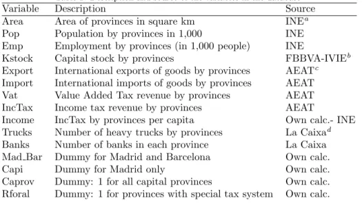
The regressors used for the aggregate model are described in Table 1. Note that the indicators should be available at the NUTS-2 and NUTS-3 level. Usu-ally, due to the data limitation problems described above, the number and quality of indicators available at this spatial level is lower than for the NUTS-2 level. However, in the Spanish case it is possible to obtain some reliable indica-tor variables that are able to proxy the GDP by the demand and supply side. All regressors enter in log levels to explain GDP (NUTS-2) for the year 2004
2All data and the hierarchical C-Matrix for spanish provinces are available from the authors
(or the years 2000-2004 in the panel case). The NUTS-2 GDP series were cal-culated by aggregating NUTS-3 GDP. Therefore, it is possible to compare the Chow-Lin predicted values with the actual data available. As a spatial weight matrixW = W1 we use the row normalized matrix for the inverse distances between the NUTS-3 provinces.
In addition, we have used three alternative spatial weight matrices: W2 is de-fined as the row normalized matrix for the inverse of the minimum travel time between provinces, computed by means of GIS software for the actual Spanish transport network and considering the speed and legal restrictions for trucks in Spain (from Gutierrez-Puebla et al. 2007). W3 is defined as a row normalized matrix for the interregional trade flows between the NUTS-3 provinces as well as between the NUTS-2 regions (these trade matrices come from the Spanish c-intereg database: www.c-intereg.es). W4 is defined as a the row normalized first order contiguity matrix.
6.2. Alternative specifications for the cross-section classical model
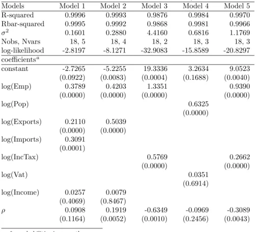
We start with the estimation of a cross-sectional SAR model and the classical Chow-Lin prediction. The first aim is to find an appropriate aggregated SAR model, using different indicator variables, which should be correlated with the ‘GDP’, both at the regional and provincial level. Table 2 shows the results obtained for the best 5 models3, using the SAR program of LeSage (1997).
The variables used in the first two models perform reasonably well, with the exception of ‘Income’. In these two models the spatial termρ is positive, but not always significant. As we will see later, these two specifications, based on the role of employment and international trade for explaining ‘GDP’ can easily be improved.
Before that, we focus on the next three models, which are characterized by the use of fiscal variables (‘Vat’, ‘IncTax’), and - surprisingly - show a negative
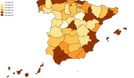
ρthat captures the spatial autocorrelation effect (although not significant for Model 4). Contrary to the intuition that spatial income effects lead to positive spillovers between neighbors, the sign obtained in these three models is negative, indicating the presence of an inverse relation between rich GDP provinces and poorer neighbors. Such a negative and significantρobtained for Model 3 and 5 can be interpreted as a form of sub-national ‘core-periphery’ structure (see Krugman, 1991) for Spanish provinces, and for some subregions, even within those. This phenomenon is a kind of a ’polycentric-periphery’ relationship, and can be seen in Figure 1, where some rich provinces like Madrid are surrounded by poor regions, and a few rich provinces are contiguous (Barcelona-Tarragona-Saragossa, Alicante-Valencia-Castell´on, Seville-C´adiz-M´alaga).
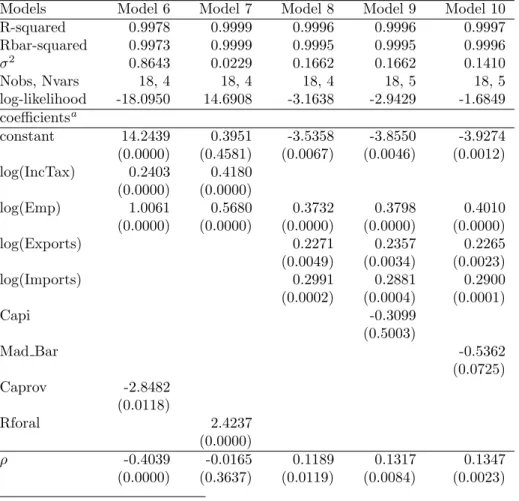
In order to test if a negative spatial correlation is generated by the ‘rich-tower-provinces’ and ‘flat-surroundings’ leading to a ‘core-periphery’ effect, we estimate two alternative specifications whose results are summarized in Table 3. In Model 6, we include a dummy variable ‘Caprov’ with 1 for capital provinces and 0 otherwise. Now, all the variables are significant and again we obtain a negative and significantρwith a much higher coefficient than in Model 5, where ‘the capital effect’ was not controlled for. However, when we move to Model 7, and the ‘Caprov’ is substituted by another dummy variable ‘Rforal’ that takes value 1 when the province belongs to an special fiscal regime within Spain and 0 otherwise, the ρ become non-significant. Thus, the cancellation of the negative and significant spatial effect in Model 7 points out to the presence of a problematic bias in the fiscal variables included (there is no alternative fiscal variables available of the same relevance and level of disaggregation). Therefore, leaving this issue for further research, we focus in three new specifications that
explore the potential of the variables included in Model 1.
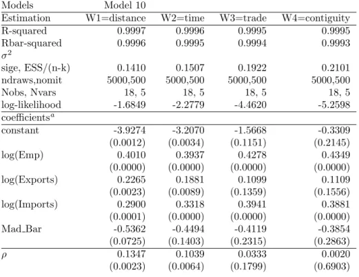
First, Model 8 consists of 3 variables (‘Employment’, international ‘Exports’ and ‘Imports’) that are able to explain by aR2 = 99.96% of the spatial dis-tribution of the ‘GDP’. Once that ‘Income’ is removed (by definition, it was also affected by the ‘fiscal bias’), all the variables are highly significant and the spatial correlation effect is positive and significant, indicating that the ‘GDP’ in a region is positively correlated with the one on their nearest neighbors. Then, in order to test if the two largest regions -‘Madrid’ and ‘Barcelona’- are causing decrements or improvements in the spatial model, we include two agglomera-tion dummy variables that take value 1 for Madrid alone (Capi) - or Madrid and Barcelona (Mad Bar), and 0 otherwise. Now, Model 9 and 10 slightly improve the results compared to Model 8. In both specifications, the agglom-eration dummy variables improve the significance of the coefficients, including the spatial term, which has higher positive coefficients and levels of significance. To explore the robustness with respect to the neighborhood matrix W, Table 4 shows the results for three alternative measures of ‘proximity’ defined in 6.1. As expected, the results for the inverse distances and travel times are very similar, obtaining high levels of significance for all variables, with the exception of the ‘Mad Bar’ dummy in the former. However, the results vary considerably when proximity is measured by ‘interregional trade’ and ‘contiguity’. In both cases, international ‘Exports’ and ‘Mad Bar’ become non-significant and the spatial effect almost disappears (low coefficients and z-values). Although this issue requires further research, it seems that the positive spatial autocorrelation effect acts in a middle ground between the ‘gravity relation’ explaining the Spanish interregional trade 4 and the ‘first order contiguity’ affected by the
4In previous papers (Llano et al. 2009; Requena et al. 2009), the interregional trade
in Spain has been analyzed using gravity equations and found important flows between dis-tant regions, like between Catalonia-Andalusia, Catalonia-Madrid or Madrid-Valencia. In the
’polycentric-periphery’ relationship suggested above.
6.3. Alternative methods of estimation
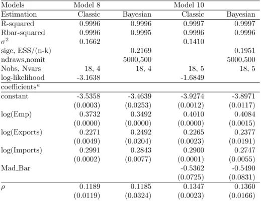
Based on Model 8 and Model 10, we estimate three additional specifications, a Bayesian cross-sectional model, a classic and a Bayesian panel model. In Table 5, we have listed the results for both specifications using classic and Bayesian cross-sectional SAR models. For both models, we obtain highR2 and levels of significance for all variables. The sign for all the variables is the right one, and theρalways have a positive coefficient within the range of 0.11 to 0.13, which is of about the same size as in Vay´a et al. (2004). Table 6 shows the results obtained for the classic and Bayesian panel SAR models. Although theR2 is
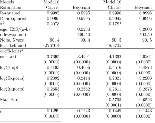
slightly lower than for the cross-section models, the level of significance for all the variables increases as well as the importance of the spatial effect, whose positive coefficients vary from 0.12 to 0.14. In all cases, the ‘Mad Bar’ variable shows negative coefficients with acceptable significance levels, pointing out to higher levels of concentration in employment and international trade in Madrid and Barcelona than in terms of ‘GDP’. Probably this result is connected with differences in productivity (GDP/employment ratios by regions) and the higher concentration of traders and headquarters in these two regions, which tends to overvalue their amount of imports and exports.
6.4. Evaluation of the spatial Chow-Lin method
The evaluation of the spatial Chow-Lin (CL) follows the evaluation methods for predictions in statistical models. This follows from the fact that unknown
y’s have to be predicted while the predictors are fully observed. In the Spanish case we are in the fortunate position of knowing the disaggregated y-values, gravity equation, proximity just explains part of the bilateral trade, and the pull and push factors linked to the origin and destination regions explain the rest.
so we can compute the prediction accuracy. This is done for the classical and Bayesian prediction as well as for the method with and without theGain (8 and 9) term. After that we compute some forecast criteria to evaluate the 4 different predictions. To evaluate the accuracy of the ML and Bayesian prediction we chose three criteria from the forecasting literature (see e.g. Chatfield, 2001): the Root Mean Squared Error (RMSE), the Mean Absolute Error (MAE) and the Mean Absolute Percentage Error (MAPE)5. The results are shown in Table 8.
According to the three criteria (RMSE, MAE and MAPE), the rankings of the models are the same. Moreover, the forecasts including the ‘gain term’, which is a function of the spatial autocorrelation, always outperform the equiv-alent methods ‘without the gain’. According to these rankings, the best method is the Bayesian cross section and panel data model ‘with gain’, followed by the classical cross-section and the classical panel model, both ‘with gain’. This shows that a spatial model will considerable improve the Chow-Lin forecasts for disaggregate data, while ignoring the spatial correlation - i.e. applying a conventional regression model instead - will lead to a considerable accuracy loss for the predicted data.
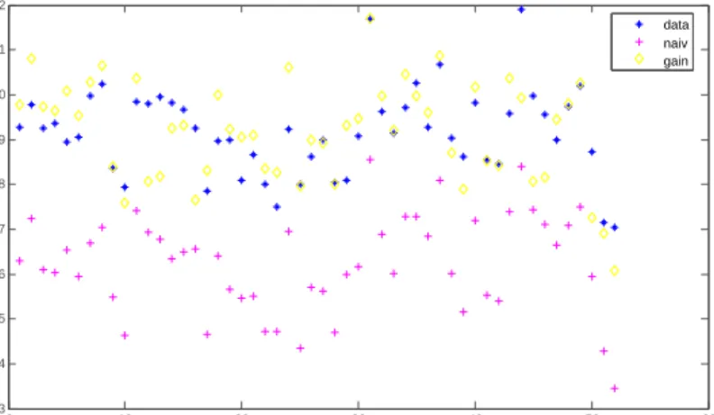
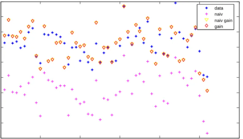
Finally, to visualize the comparisons, Figures 2 to 5 show overlay plots of the classical and Bayesian Chow-Lin predictions for model 10, with and without gain, together with the observed data, using the cross-sectional and the panel data specification. Figures 3 and 5 show clearly that the Bayesian spatial Chow-Lin forecasts lie closer to the observed values than classical predictions or non-spatial methods (denoted as ’no gain’) in Figure 4.
5The formulas areRM SE= 1
N q PN i=1(y−by) 2,M AE= 1 N PN i=1|y−by|andM AP E= 1 N PN i=1| y−yb y |respectively.
7. Conclusions
Regional econometric work in Europe has become increasingly important, especially since the integration process of the European Union puts a lot of weight on policies for regional coherence. For such evaluations NUTS data are the main source of information. They are collected by Eurostat and the individual member states using common rules and methods. But not all member states have developed the same level of skills, especially since 1995 after the harmonized European national accounting system has started. This leads to inhomogeneous data quality and sometimes to holes in the database if smaller regional units are needed. In order to apply many modern panel methods one has to complete such data sets. While the simplest method is interpolation, this gives not always satisfactory results.
In this study, we develop a new spatial Chow-Lin procedure similar to the original one used in the field of time series interpolation. The procedure uses the indicators at the disaggregated regional level to predict the disaggregated un-observed dependent variable, conditional on the complete aggregated un-observed model. We showed that the spatial Chow-Lin method can be formulated in a Bayesian framework and can be also used for completing data in a spatial panel model.
To evaluate the new method, we forecasted the GDP for the 52 Spanish provinces (at NUTS-3 level), but based only on the information for the 18 Spanish regions (i.e. NUTS-2 GDP as dependent variable), while the forecasts are based on high frequency socio-economic indicators at the NUTS-3 level. Then, to compare the results obtained with the actual series available at the NUTS-3 level, we computed forecast criteria. Interestingly, we found models also with a significant negative spatial autocorrelation effects by including the fiscal variable ‘Income Tax’, but the R2 fit is lower than for models with positive
rhos’s. Moreover, the Chow-Lin results improve if we control for the centers Madrid and Barcelona, because spatial spillovers are sensitive to the definition of the spatial neighborhood matrices and the concept of ‘proximity’.
Finally, we point out that a significant spatial lag parameter leads to an improvement (through the so called gain term) in the spatial Chow-Lin predic-tion of the disaggregated data. The Bayesian MCMC method yield the best result among the 10 models in the forecast experiment. This seems to be true for the Bayesian and classical estimation methods or cross-sectional and panel data. Our new method has shown that it pays to get a good spatial model if one is interested in good predictions of missing data in a cross-sectional or panel model. A non-trivial condition for finding a good model is the existence of good indicators, the removal of outliers and the skill to find the appropriate weight matrix to estimate the spatial effects. In future research we will explore these modeling possibilities in more detail and extend the spatial Chow-Lin method to complete large blocks of data at the national and European level, including flow data such as inter-regional trade or migration flows.
References
Anselin, L., 1988. Spatial Econometrics: Methods and Models. Dordrecht: Kluwer Academic Publishers.
Boot, J. C. G., Feibes, W., Lisman, J. H., 1967. Further methods of derivation of quarterly figures from annual data. Applied Statistics 16, 65–75.
Chatfield, C., 2001. Time-series Forecasting. Chapman & Hall.
Chow, G. C., Lin, A., 1971. Best linear unbiased interpolation, distribution, and extrapolation of time series by related series. The Review of Economics and Statistics 53 (4), 372–375.
Denton, F., 1971. Adjustment of monthly or quarterly series to annual totals: An approach based on quadratic minimization. Journal of American Statistical Association 66, 99–102.
Di Fonzo, T., 1990. The estimation of m disaggregate time series when contem-poraneous and temporal aggregates are known. The Review of Economics and Statistics 71, 178–182.
Duranton, G., Overman, H., October 2005. Testing for localization using micro-geographic data. Review of Economic Studies 4, 1077–1106.
Duranton, G., Overman, H. G., February 2008. Exploring the detailed location patterns of u.k. manufacturing industries using microgeographic data. Journal of Regional Science 48 (1), 213–43.
Fernandez, R. B., 1981. A methodological note on the estimation of time series. The Review of Economics and Statistics 53, 471–478.
Friedman, M., 1962. The interpolation of time series by related series. Journal of American Statistical Association 57, 729–757.
Guttorp, P., Meiring, W., Sampson, P., 1994. A space-time analysis of ground-level ozone data. Environmetrics 5, 241–254.
Helliwell, J. F., Verdier, G., 2000. Measuring internal trade distances: a new method applied to estimate provincial border effects in canada. Canadian Journal of Economics 34 (4), 1024–1041.
Hillberry, R., August 2002. Aggregation bias, compositional change, and the border effect. Canadian Journal of Economics 35 (3), 517–530.
Huerta, G., Sanso, B., Stroud, J. R., 2004. A spatiotemporal model for mexico city ozone levels. Applied Statistics 53 (2), 231–248.
Krugman, P. R., 1991. Increasing returns and economic geography. Journal of Political Economy 99, 183 – 199.
Kyriakidis, P. C., Yoo, E.-H., 2005. Geostatistical prediction and simulation of point values from areal data. Geography Analysis 37 (2), 124–151.
LeSage, J. P., 1997. Bayesian estimation of spatial autoregressive models. Inter-national Regional Science Review 20, 113–129.
LeSage, J. P., Pace, R. K., 2004. Models for spatially dependent missing data. Journal of Real Estate Finance and Economics 29, 233–254.
Litterman, R. B., 1983. A random walk, markov model for the distribution of time series. Journal of Business and Economic Statistics 1, 169–173.
OECD, 1996. Sources and methods used by the oecd member countries. Tech. rep., Quarterly National Accounts. OECD: Paris.
Pavia-Miralles, J. M., Cabrer-Borras, B., 2007. On estimating contemporaneous quarterly regional gdp. Journal of Forecasting 26, 155–170.
Pavia-Miralles, J. M., Vila-Lladosa, L.-E., Valles, R. E., 2003. On the perfor-mance of the chow-lin procedure for quarterly interpolation of annual data: Some monte-carlo analysis. Spanish Economic Review 5, 291–305.
Poncet, S., 2003. Measuring chinese domestic and international integration. China Economic Review 14 (1), 1–21.
Poncet, S., 2005. A fragmented china, measure and determinants of chinese domestic market disintegration. Review of International Economics 13 (3), 409–430.
Vay´a, E., L´opez-Bazo, E., Moreno, R., Art´ıs, M., 2004. Growth and external-ities across economies: an empirical analysis using spatial econometrics. In: Anselin, L., Florax, R., Rey, S. (Eds.), Advances in spatial econometrics: methodology, tools and applications. Advances in spatial Sicence. Springers. Yoo, E.-H., Kyriakidis, P. C., 2006. Area-to-point kriging with inequality-type
8. Tables and Figures
Table 1: Description and source of the variables in the database
Variable Description Source
Area Area of provinces in square km INEa Pop Population by provinces in 1,000 INE Emp Employment by provinces (in 1,000 people) INE
Kstock Capital stock by provinces FBBVA-IVIEb
Export International exports of goods by provinces AEATc Import International imports of goods by provinces AEAT Vat Value Added Tax revenue by provinces AEAT IncTax Income tax revenue by provinces AEAT
Income IncTax by provinces per capita Own calc.- INE Trucks Number of heavy trucks by provinces La Caixad
Banks Number of banks in each province La Caixa Mad Bar Dummy for Madrid and Barcelona Own calc.
Capi Dummy for Madrid only Own calc.
Caprov Dummy: 1 for all capital provinces Own calc. Rforal Dummy: 1 for provinces with special tax system Own calc.
awww.ine.es
bwww.fbbva.es,www.ivie.es cwww.aeat.es
Table 2: Cross sectional SAR model: classic estimates for GDP 2004, NUTS-2 and NUTS-3
Models Model 1 Model 2 Model 3 Model 4 Model 5
R-squared 0.9996 0.9993 0.9876 0.9984 0.9970 Rbar-squared 0.9995 0.9992 0.9868 0.9981 0.9966 σ2 0.1601 0.2880 4.4160 0.6816 1.1769 Nobs, Nvars 18, 5 18, 4 18, 2 18, 3 18, 3 log-likelihood -2.8197 -8.1271 -32.9083 -15.8589 -20.8297 coefficientsa constant -2.7265 -5.2255 19.3336 3.2634 9.0523 (0.0922) (0.0083) (0.0004) (0.1688) (0.0040) log(Emp) 0.3789 0.4203 1.3351 0.9390 (0.0000) (0.0000) (0.0000) (0.0000) log(Pop) 0.6325 (0.0000) log(Exports) 0.2110 0.5039 (0.0000) (0.0000) log(Imports) 0.3091 (0.0001) log(IncTax) 0.5769 0.2662 (0.0000) (0.0000) log(Vat) 0.0351 (0.6914) log(Income) 0.0257 0.0079 (0.4069) (0.8467) ρ 0.0908 0.1919 -0.6349 -0.0969 -0.3089 (0.1164) (0.0052) (0.0010) (0.2456) (0.0043) az-probabilities in parentheses
Table 3: Cross-sectional SAR model: classic estimates for GDP, 2004 (NUTS-2 and NUTS-3) Models Model 6 Model 7 Model 8 Model 9 Model 10
R-squared 0.9978 0.9999 0.9996 0.9996 0.9997 Rbar-squared 0.9973 0.9999 0.9995 0.9995 0.9996 σ2 0.8643 0.0229 0.1662 0.1662 0.1410 Nobs, Nvars 18, 4 18, 4 18, 4 18, 5 18, 5 log-likelihood -18.0950 14.6908 -3.1638 -2.9429 -1.6849 coefficientsa constant 14.2439 0.3951 -3.5358 -3.8550 -3.9274 (0.0000) (0.4581) (0.0067) (0.0046) (0.0012) log(IncTax) 0.2403 0.4180 (0.0000) (0.0000) log(Emp) 1.0061 0.5680 0.3732 0.3798 0.4010 (0.0000) (0.0000) (0.0000) (0.0000) (0.0000) log(Exports) 0.2271 0.2357 0.2265 (0.0049) (0.0034) (0.0023) log(Imports) 0.2991 0.2881 0.2900 (0.0002) (0.0004) (0.0001) Capi -0.3099 (0.5003) Mad Bar -0.5362 (0.0725) Caprov -2.8482 (0.0118) Rforal 2.4237 (0.0000) ρ -0.4039 -0.0165 0.1189 0.1317 0.1347 (0.0000) (0.3637) (0.0119) (0.0084) (0.0023) az-probabilities in parentheses
Table 4: Cross-sectional SAR model: classic and Bayesian estimates. GDP, 2004
Models Model 10
Estimation W1=distance W2=time W3=trade W4=contiguity
R-squared 0.9997 0.9996 0.9995 0.9995 Rbar-squared 0.9996 0.9995 0.9994 0.9993 σ2 sige, ESS/(n-k) 0.1410 0.1507 0.1922 0.2101 ndraws,nomit 5000,500 5000,500 5000,500 5000,500 Nobs, Nvars 18, 5 18, 5 18, 5 18, 5 log-likelihood -1.6849 -2.2779 -4.4620 -5.2598 coefficientsa constant -3.9274 -3.2070 -1.5668 -0.3309 (0.0012) (0.0034) (0.1151) (0.2145) log(Emp) 0.4010 0.3937 0.4278 0.4349 (0.0000) (0.0000) (0.0000) (0.0000) log(Exports) 0.2265 0.1881 0.1099 0.1109 (0.0023) (0.0089) (0.1359) (0.1556) log(Imports) 0.2900 0.3318 0.3941 0.3881 (0.0001) (0.0000) (0.0000) (0.0000) Mad Bar -0.5362 -0.4494 -0.4119 -0.3854 (0.0725) (0.1403) (0.2315) (0.2863) ρ 0.1347 0.1039 0.0333 0.0020 (0.0023) (0.0064) (0.1799) (0.6903)
Table 5: Cross-sectional SAR model: classic and Bayesian estimates. GDP, 2004
Models Model 8 Model 10
Estimation Classic Bayesian Classic Bayesian
R-squared 0.9996 0.9996 0.9997 0.9997 Rbar-squared 0.9996 0.9995 0.9996 0.9996 σ2 0.1662 0.1410 sige, ESS/(n-k) 0.2169 0.1951 ndraws,nomit 5000,500 5000,500 Nobs, Nvars 18, 4 18, 4 18, 5 18, 5 log-likelihood -3.1638 -1.6849 coefficientsa constant -3.5358 -3.4639 -3.9274 -3.8971 (0.0003) (0.0253) (0.0012) (0.0117) log(Emp) 0.3732 0.3492 0.4010 0.4084 (0.0000) (0.0000) (0.0000) (0.0015) log(Exports) 0.2271 0.2492 0.2265 0.2377 (0.0049) (0.0204) (0.0023) (0.0191) log(Imports) 0.2991 0.2843 0.2900 0.2747 (0.0002) (0.0077) (0.0001) (0.0055) Mad Bar -0.5362 -0.5490 (0.0725) (0.0831) ρ 0.1189 0.1185 0.1347 0.1360 (0.0119) (0.0324) (0.0023) (0.0166)
Table 6: Panel data SAR models: GLS and Bayesian estimates for GDP, 2000-2004
Models Model 8 Model 10
Estimation Classic Bayesian Classic Bayesian
R-squared 0.9995 0.9995 0.9996 0.9995 Rbar-squared 0.9995 0.9995 0.9995 0.9995 σ2 0.2073 0.1782 sige, ESS/(n-k) 0.2230 0.2003 ndraws,nomit 500,50 500,50 Nobs, Nvars 90, 4 90, 4 90, 5 90, 5 log-likelihood -25.7614 -18.9705 coefficientsa constant -3.7695 -3.4991 -4.1362 -4.0264 (0.0000) (0.0000) (0.0000) (0.0000) log(Emp) 0.4193 0.4066 0.4516 0.4873 (0.0000) (0.0000) (0.0000) (0.0000) log(Exports) 0.2392 0.2414 0.2321 0.2208 (0.0000) (0.0000) (0.0000) (0.0000) log(Imports) 0.2653 0.2662 0.2611 0.2576 (0.0000) (0.0000) (0.0000) (0.0000) Mad Bar -0.5765 -0.6526 (0.0001) (0.0000) ρ 0.1299 0.1223 0.1449 0.1443 (0.0000) (0.0000) (0.0000) (0.0000) az-probabilities in parentheses
Table 7: Chow-Lin Prediction Accuracy: Classical vs. Bayesian estimates
RMSEa MAEb MAPEc
Cross-section Classical gain 1.242 0.098 0.905
no gain 1.338 0.140 1.285
Bayesian gain 0.820 0.067 0.618
no gain 2.930 0.321 2.905
Panel-data Classical gain 3.166 0.348 3.146
no gain 3.209 0.352 3.187
Bayesian gain 0.822 0.067d 0.621
no gain 3.100 0.340 3.078
aRoot Mean Squared Error bMean Absolute Error
cMean Absolute Percentage Error dMinimum
Figure 1: Geographical distribution of GDP 2004 for the Spanish provinces (NUTS-3)
Figure 2: Overlay Comparison: Classical cross-sectional GDP predictions with and without gain across NUTS-3 regions
0 10 20 30 40 50 60 5 6 7 8 9 10 11 12 13 14 Disaggregate Values data naiv naiv gain gain
Figure 3: Overlay Comparison: Bayesian cross-section predictions with and without gain and across NUTS-3 regions
0 10 20 30 40 50 60 3 4 5 6 7 8 9 10 11 12 Disaggregate Values data naiv gain
Figure 4: Overlay Comparison: Classical panel-data predictions with and without gain across NUTS-3 regions 0 10 20 30 40 50 60 3 4 5 6 7 8 9 10 11 12 Disaggregate Values data naiv naiv gain gain
Figure 5: Overlay Comparison: Bayesian panel-data predictions with and without gain across NUTS-3 regions 0 10 20 30 40 50 60 3 4 5 6 7 8 9 10 11 12 Disaggregate Values data naiv naiv gain gain