Cluster-Based Estimators For Multiple And Multivariate Linear Regression Models

CLUSTER-BASED ESTIMATORS FOR

MULTIPLE AND MULTIVARIATE LINEAR

REGRESSION MODELS

EKELE ALIH

UNIVERSITI SAINS MALAYSIA

2015

CLUSTER-BASED ESTIMATORS FOR

MULTIPLE AND MULTIVARIATE LINEAR

REGRESSION MODELS

by

EKELE ALIH

Thesis submitted in fulfilment of the requirements

for the degree of

Doctor of Philosophy

DEDICATIONS

Anabel-Martha Ugbedeojo, Mummy’s death has made you unstable– I just wish I can make up for you upon my return

Gabriel-AkoEkele, Daddy left you to study just few hours after you came–I just hope you will recognize me when I return

ACKNOWLEDGEMENTS

I give honour, thanks, gratitude and appreciation to the Creator God for bringing me

into this world, for being with me in times of trouble, for providing all my needs and

above all for giving me sound wisdom, knowledge and understanding even in the face

of uncertainties in the course of this Doctorate Degree Programme.

My special appreciation goes to Associate Professor Hong Choon Ong, who welcomed

me like a father will welcome a son when I arrived in Malaysia; who guided me like a

father will guide his son during my registration process to be a PhD student of USM;

who provided for me, all I needed to do in my research when I eventually settled down

as a PhD student of PPSM, USM; who took all the pains to go through every line of this

Thesis and offered suggestions and corrections. I sincerely thank him for condoning

all my acts, both ‘the good’, ‘the bad’ and ‘the ugly’ and for heartily moderating this research project to its peak. Once, again, Remain blessed, Prof. Ong.

I thank my Parents, Mr. Stephen Ibrahim Alih and Mrs. Martha Ibrahim Alih, through

whom I came into this world. They have persistently been praying for my success and

hope to celebrate my victory in this PhD journey. Thank you, ‘MUM&DAD’.

My wife made sacrifices in no small measure in the course of my PhD pursuit. One of

those sacrifices was to allow me to travel for the PhD program barely 8 days after you

underwent a caesarian operation that gave birth to our boy, Gab. You borne the pains

is love at its peak. These gestures are indelible in my mind. Thank you, Stella-Gbelei.

The Federal Polytechnic Idah is immensely appreciated for providing my funding

through the TETFUND of the Federal Republic of Nigeria. Thank you to the

Gov-ernment of ‘myfatherland’

I appreciate my two kids, Anabel and Gabriel, who missed me dearly and whom I

dearly missed while I am away to pursue the PhD. I love you and will soon join you as

we hope to grow together in God’s path.

Colleagues and staff of Maths/Statistics Department, Federal Polytechnic Idah are also

acknowledged for their co-operation with me while pursuing the programme. Thank

you all.

Above all, I thank once more the Almighty God for His unquantifiable journey mercies

and for sustaining my life all through the period of study. Once again, I acknowledge

that I am divinely favoured.

Ekele Alih

TABLE OF CONTENTS

Acknowledgements ii

Table of Contents iv

List of Tables ix

List of Figures xii

List of Abbreviations xiv

List of Symbols xviii

List of Publications xxiii

Abstrak xxv

Abstract xxvii

CHAPTER 1 –INTRODUCTION

1.1 General Introduction 1

1.2 Motivation of the Study 3

1.3 Research Objectives 5

1.4 Thesis Organization 6

1.5 Regression background and Notation 6

1.6 The Least squares Regression-LS 10

1.6.1 Terminology 11

1.7 Leverage and the Hat Matrix 13

1.7.1 Altered Hat Matrix 15

1.8 Outlier Diagnostics 16

1.9 Influence Diagnostics 18

2.1 Introduction 20

2.2 Location and Dispersion Estimators 22 2.2.1 The Forward Search Procedures 23

2.2.1(a) The Stahel-Donoho Estimator 23 2.2.1(b) The Stalactite Plot Analysis 25

2.2.1(c) The Orthogonalized Gnanadesikan-Kettenring Estimator 27

2.2.1(d) TheBACON: Block Adaptive

Computationally-Efficient Outlier Nominators 29

2.2.2 The Elemental or Resampling Procedures 32 2.2.2(a) The Minimum Volume Ellipsoid Estimator for

Location and Dispersion in the presence of Outliers 32

2.2.2(b) The Minimum Covariance Determinant Estimator for

Location and Dispersion in the presence of Outliers 36

2.2.2(c) The Deterministic Minimum Covariance Determinant

(DetMCD)Estimator for Location and Dispersion in

the presence of Outliers 39

2.3 Robust Estimators for Multiple Linear Regression Analysis 43

2.3.1 Low Breakdown Regression Estimators 44 2.3.2 M and Bounded Influence Regression 45

2.3.3 High Breakdown Regression Estimators 49 2.4 Multivariate Linear Regression Analysis 53

2.4.1 Robust estimation in Simultaneous equation models 55

2.4.2 The MCD Robust Multivariate Regression (MCDreg) 56 2.4.3 The Multivariate RegressionS-estimators (MSreg) 57 2.4.4 The Multivariate Least-trimmed Square Estimator (MLTSreg) 59

CHAPTER 3 –THE PROPOSED MULTIVARIATE OUTLIER IDENTIFICATION WITH ITS LOCATION AND DISPERSION ESTIMATOR

3.2 The Proposed MMD Forward Search Algorithm Estimator 67

3.2.1 Definition of MMD Estimator 69 3.3 The Rationale of MMD Algorithm Estimator 73

3.4 Numerical Illustration and Monte Carlo Simulation Experiment 75 3.4.1 Artificial Dataset Illustration 75

3.4.2 Dilemma Dataset Illustration 78

3.4.3 Monte Carlo Simulation Experiment 83 3.5 Equivariance, Robustness and Efficiency Properties of MMD 87

3.5.1 Equivariance Properties 88

3.5.2 Numerical Equivariance 90

3.5.3 Breakdown Value (Robustness) of MMD Estimator 92

3.5.4 Finite Sample Efficiency 94

CHAPTER 4 –THE PROPOSED UNIVARIATE SIMPLE AND MULTIPLE REGRESSION PROCEDURE

4.1 Introduction 98

4.1.1 The Concentration Steps Algorithm 100

4.1.2 The Concept of Cluster Analysis 102 4.2 The Proposed Cluster-based L2 Robust Regression-CL2RR 106

4.2.1 TheC-step Phase 107

4.2.1(a) Definitions 107

4.2.1(b) TheCL2RRInitial Estimator Algorithm 110 4.2.2 The Sequential Regression Phase 112 4.2.3 TheCL2RRNumerical Demonstration 118 4.2.3(a) Analysis ofCL2RRInferences 126 4.2.3(b) Empirical Assessment ofCL2RRInferences 127 4.3 Numerical Example and Monte Carlo Simulation 130

4.3.1 The Stackloss Data set 130

4.3.2 The Pendleton and Hocking Data set 134 4.3.3 Monte Carlo Simulation Experiment 137

4.4 Robustness and Equivariance Properties of CL2RR 144 4.4.1 Robustness properties of CL2RR 144

4.4.2 Equivariance properties of CL2RR 146

4.5 Chapter Summary and Conclusion 148

4.5.1 Summary 148

4.5.2 Conclusion 149

CHAPTER 5 –THE PROPOSED CLUSTER-BASED MULTIVARIATE REGRESSION PROCEDURE

5.1 Introduction 151

5.2 The Proposed Cluster-based Multivariate Robust Regression-CMRR 152

5.2.1 Definitions 152

5.2.2 Robustness properties 157

5.3 CMRR Algorithm 158

5.3.1 TheCMRRNumerical Demonstration 161 5.3.2 Analysis ofCMRRInferences 170 5.4 Numerical Example and Monte Carlo Simulation 171 5.4.1 The Pulp-fibre Data set 171

5.4.2 The Milk Data set 181

5.4.3 Monte Carlo Simulation 188 5.4.4 Finite Sample Efficiency 195

5.5 Summary 196

6.2 Current Regression Methodologies 199

6.2.1 The Ordinary Least Squares 199

6.2.2 The M-regression 200

6.2.3 The Bounded Influence Regression 200 6.2.4 The Least Median of Squares Regression 200

6.2.5 The Least Trimmed Squares Regression and Least Trimmed

Absolute Value Regression 201

6.2.6 TheMMRegression 201

6.2.7 Findings and Contribution of This Thesis 202 6.2.8 Recommendations for Future Research 203

References 205

APPENDICES 210

A.1 R programming Code for Outlier Identification and Computation of

Location and Dispersion Estimator via theMMDAlgorithm. 211 B.1 R programming Code for theCL2RRNumerical Demonstration 216 C.1 R programming Code for theCMRRNumerical Demonstration 231

LIST OF TABLES

Page

Table 3.1 Artificial Dataset 76

Table 3.2 Robust Mahalanobis Distances ofMMD,MV E,DetMCDand

BACON estimators for Artificial Dataset 77

Table 3.3 Dilemma Dataset 79

Table 3.4 Robust Mahalanobis Distances ofMMD,MV E,DetMCDand

BACON estimators for Dilemma Dataset 81

Table 3.5 Performance Evaluation ofMMD,MV E,DetMCDandBACON

estimators for Dilemma Dataset 82

Table 3.6 Monte Carlo Performance Evaluation ofMMD,MV E,

DetMCDandBACON estimators 85

Table 3.7 Simulation results of Deviation from Affine Equivariance,

dCL2RR ofCL2RR 91

Table 3.8 Finite Sample Efficiency of theMMDestimators 95

Table 4.1 Simulated simple linear regression data 119

Table 4.2 The pivot point estimate,BfromLS-regression. 121

Table 4.3 Similarity matrix computed from

si j = (bi−bj)′(CD(B))−1(bi−bj) 122

Table 4.4 CL2RR Parameter estimates, Other Competitors and the True

Parameter Values 125

Table 4.5 CL2RR Analysis of Variance 127

Table 4.6 Monte Carlo Performance Evaluation on the CL2RR Inferential

Statistics 129

Table 4.7 The Stackloss Dataset 131

Table 4.8 A Summary ofCL2RREstimation and Robust ANOVA for

Stackloss Data set 133

Table 4.10 A Summary ofCL2RREstimation and Robust ANOVA for

Pendleton and Hockings Dataset 136

Table 4.11 Simulation result of estimators’ performances atd=0%(i.e. no

outlier) 139

Table 4.12 Simulation result of estimators’ performances atd=20% 140

Table 4.13 Simulation result of estimators’ performances atd=30% 140

Table 4.14 Simulation result of estimators’ performances atd=50% 141

Table 5.1 Multivariate Regression Artificial Data 163

Table 5.2 Mahalanobis distance fromMMDestimator 164

Table 5.3 Mahalanobis distance of residualsd_i2(βββˆ,ΣΣΣmˆ )and its rankR_d 165

Table 5.4 Mahalanobis distance of residualsd_i2(βββˆ,ΣΣΣmˆ )and its rankRd at

convergence of Steps 1 and 2 166

Table 5.5 The Leverage Weightsπππ(di) 168

Table 5.6 CMRR Analysis of Variance 171

Table 5.7 The Pulp-fibre Dataset 172

Table 5.8 CMRRParameter Estimates and Inferential Statistics for Pulp

Fibre Data 176

Table 5.9 MSregParameter Estimates and Inferential Statistics for Pulp

Fibre Data 177

Table 5.10 MLT SregParameter Estimates and Inferential Statistics for

Pulp Fibre Data 178

Table 5.11 MCDregParameter Estimates and Inferential Statistics for Pulp

Fibre Data 178

Table 5.12 The Milk Dataset 181

Table 5.13 CMRRParameter Estimates and Inferential Statistics for the

Milk Data 186

Table 5.14 MSregParameter Estimates and Inferential Statistics for the

Milk Data 187

Table 5.15 MLT SregParameter Estimates and Inferential Statistics for the

Table 5.16 MLT SregParameter Estimates and Inferential Statistics for the

Milk Data 188

Table 5.17 Simulation results of Bias of Coefficient Matrix 191

Table 5.18 Simulation results of MSE of Coefficient Matrix 191

Table 5.19 Simulation results of Computing Time(t in sec.)of Coefficient

Matrix 192

LIST OF FIGURES

Page

Figure 1.1 Scatter Plot Illustrating Outliers and Leverages 12

Figure 3.1 Index Plot of Location and Dispersion Estimator for Artificial Dataset: (a) Index Plot of MMD Estimator (b) Index Plot of MVE Estimator (c) Index Plot of DetMCD Estimator and (d)

Index Plot of BACON Estimator. 77

Figure 3.2 Index Plot of Location and Dispersion Estimator for Dilemma Dataset: (a) Index Plot of MMD Estimator (b) Index Plot of MVE Estimator (c) Index Plot of DetMCD Estimator and (d)

Index Plot of BACON Estimator. 82

Figure 3.3 Line Plots of Percentage Detection Rates for MMD, MVE,

DetMCD and BACON Estimators. 86

Figure 3.4 Line Plots of Percentage Swamping Rates for MMD, MVE,

DetMCD and BACON Estimators. 87

Figure 3.5 Line Plots ofMMDefficiency 96

Figure 4.1 Dendrogram Plot of Simple Linear Regression Data. 122

Figure 4.2 The FF Plot of Linear Regression Fits forOLS,LT S,MM,CBI,

andCL2RR 125

Figure 4.3 Regime Plot of computation time for Simulated Data: (bi) Time plot at zero percentage outlier(d=0%), (bii) Time plot at

d=20% outlier (biii) Time plot atd=30% outlier, and (biv)

Time plot atd=50% outlier 142

Figure 4.4 Regime Plot of bias for Simulated Data: (ai) Bias plot at zero percentage outlier(d=0%), (aii) Bias plot atd=20% outlier (aiii) Bias plot atd=30% outlier, and (aiv) Bias plot at

d=50% outlier 143

Figure 5.1 Dendrogram Plot of Multivariate Linear Regression Data. 167

Figure 5.2 Dendrogram Plot of Pulp Fibre Data. 175

Figure 5.4 Dendrogram Plot of Milk Data. 186

Figure 5.5 Regime Plot of Bias for Simulated Data: (ai) Bias plot at zero percentage outlier(d=0%), (aii) Bias plot atd=20% outlier (aiii) Bias plot atd=30% outlier, and (aiv) Bias plot at

d=40% outlier 193

Figure 5.6 Regime Plot of computing time for Simulated Data: (bi) Time plot at zero percentage outlier(d=0%), (bii) Time plot at

d=20% outlier (biii) Time plot atd=30% outlier, and (biv)

LIST OF ABBREVIATIONS

3SLS 3 Stage Least Squares

AHC Agglomerative Hierarchical Clustering

ANOVA Analysis-of-Variance

BACON Block Adaptive Computationally-efficient Outlier Nominator

BDP Break Down Point

BI Bounded Influence

BIR Bounded Influence Regression

BLUE Best Linear Unbiased Estimator

CBI Cluster-Based Bounded Influence Regression

C-Step Concentration Steps

CL2RR Cluster-based L2 Robust Regression

CLreg Cluster-based Estimator for Multiple and Multivariate Linear Regression

CMRR Cluster-based Multivariate Robust Regression

det Determinant of a Matrix

DetMCD Deterministic Minimum Covariance Determinant

df Degree of Freedom

DFFITS Difference in Fits influence diagnostics

DFFITSi Difference in Fits influence diagnostics whenith observation has been

removed

DFFITSl Difference in Fits influence diagnostics when the set oflobservations has

been removed

DHC Divisive Hierarchical Clustering

FastMCD Fast Minimum Covariance Determinant

FSA Forward Search Algorithm

GM Generalized Maximum Likelihood Estimator

iid Independently and identically distributed

IRLS Iteratively Reweighted Least Squares

LAD Least Absolute Deviation

LS Least Squares

LTA Least Trimmed Absolute Deviation

LTS Least Trimmed Squares

M A type of Maximum Likelihood Estimator

MAD Median Absolute Deviation

MCD Minimum Covariance Determinant

MCDreg Minimum Covariance Determinant Regression

MLR Multiple Linear Regression

MVE Minimum Volume Ellipsoid

MLE Maximum Likelihood Estimator

MLTSreg Multivariate Least Trimmed Squares Regression

MM A type of Maximum Likelihood Estimator in two phases

MMD Minimum Mahalanobis Distance Algorithm

MSreg Mean Squared Regression

MSres Mean Squared Residuals

MSreg Multivariate Scale Regression

OLS Ordinary Least Squares

OLSWO Ordinary Least Squares when observations identified as outliers have been removed from the dataset

PDS Positive Definite and Symmetric Matrix

PRESS Prediction Residuals

RD Robust Distances

REWLS Reweighted Least Squares

SSE Sum of Square Error

SLR Simple Linear Regression

SS Sum of Squares

SSreg Sum of Squares Regression

LIST OF SYMBOLS

α Level of significance

βββ Regression parameters

βj Element ofβββ relating to the jthregressor

ˆ

β_ββˆˆ _{An estimate ofβββ} ˆ

βj Element of ˆβββˆˆ relating to the jthregressor C Covariance matrix

⌈ ⌉ Ceil: Rounds up a float to a specified number of decimal places

Cℓ MMD’s covariance matrix

Cm Main cluster

C_τ Minor cluster

Chm Main cluster containing onlyhobservations CJ Covariance matrix ofJthsubsample

δ cutoff value for a diagnostic statistic

di(.) Theith Mahalanobis distance of an argument εεε Random error matrix

εi Theithrandom error

f(.) Model function

∀ For all

γ Breakdown point, i.e. fraction of outlier that an estimator can tolerate

H Hat matrix

h Number of observations defining a half dataset of data

hii Theithdiagonal ofH

hi j Theithrow and the jthcolumn element ofH Hy The altered hat matrix

J Subsample size

Jm Initial sample

l Size of minor clusters to be activated

L1 Least absolute deviation regression loss function

m Mean vector

˜

m Median vector

mℓ MMD’s mean vector

m Size of initial Sample or Initial subset

mJ Mean vector ofJth subsample

µµµ Population Mean ˆ µˆ µµˆ Estimate ofµµµ MMD(βββ) MMD-variance N Population size n Number of observations

p Number of predictor variables

# Paired sample with parallel and equal size

q Number of response variables

Rstudenti The Studentizedt-like diagnostics r Residual vector

ri,−i Residual values atx

′

iwhenithobservation is removed σσσ2 _{Vector of variances}

σσσ Vector of standard deviations

ΣΣΣ Population covariance matrix ˆ

Σ_ΣΣˆˆ _{Estimate ofΣΣΣ}

s Root mean square error forOLSregression

s_−i Root mean square error forOLSregression whenith observation is removed

ui Robust projection distances

v Direction vector ofk×1 or p×1 dimension

x Predictor variable of interest

xi Theithpredictor variable

xji Theithobservation for the jthpredictor X Predictor matrix including intercept

x′_i Theithrow ofX

Xy Predictor matrix with intercept and augmented with the response vector

y Response variable of interest

yi Theithresponse variable

yi,−i Fitted values atx

′

iwhenithobservation is removed

yki Theithobservation for thekthresponse ˆy Predicted response vector

Z Predictor matrix excluding intercept

z′_i Theithrow ofZ

LIST OF PUBLICATIONS

LIST OF PUBLICATIONS

[1] Alih, E., and Ong, H. C., (2015), Robust Cluster-Based Multivariate Outlier Di-agnostics and Parameter Estimation in Regression Analysis,Communications in Statistics - Simulation and Computation, Accepted: DOI 10.1080/036

10918.2014.960093. [ISI Impact Factor:0.288]

[2] Alih, E., and Ong, H. C., (2015), An Outlier-resistant Test for Heteroscedasticity in Linear Models, Journal of Applied Statistics, 42:8, 1617-1634. [ISI Impact Factor: 0.656 ].

[3] Alih, E., and Ong, H. C., (2015), Cluster-based Multivariate outlier identification and Re-weighted Regression in Linear Models, Journal of Applied Statistics,

42:5, 938-955. [ISI Impact Factor: 0.656].

[4] Alih, E., and Ong, H. C., An Outlier resistant algorithm of T2 Control Chart for Skewed Population, Statistical Methods & Applications, Under Review. [ISI Impact Factor: 0.571].

[5] Alih, E., and Ong, H. C., Cluster-based L2 Re-weighted Regression, Statistical Methodology, Accepted: DOI 10.1016/j.stamet.2015.05.005. [ISI Impact Fac-tor: 0.708].

[6] Ong, H. C., and Alih, E., Cluster-based Multivariate Regression,Pakistan Journal of Statistics, Accepted. [ISI Impact Factor: 0.336].

[7] Ong, H. C., and Alih, E.,(2015), A Control Chart Based on Cluster-Regression Adjustment for Retrospective of Monitoring Individual Characteristics, PLoS One,10(4):e0125835. [ISI Impact Factor: 3.534].

[8] Alih, E., and Ong, H. C., (2014), The performance of robust multivariate regres-sion in simultaneous dependence of variables in linear models,AIP Conference Proceedings,1606, pp 1028-1033.

[9] Alih, E., and Ong, H. C., (2015), Cluster-based Control Chart Method, National Symposium on Mathematical Sciences (SKSM22) Shah Alam, Kuala Lumpur.

PENGANGGAR BERASASKAN

KELOMPOK BAGI MODEL REGRESI

BERGANDA DAN LINEAR MULTIVARIAT

ABSTRAK

Dalam bidang pemodelan regresi linear, regresi kuasa dua terkecil (LS) klasik adalah

mudah dipengaruhi oleh titik terpencil manakala penganggar regresi rendah-kerosakan

seperti regresi M dan regresi pengaruh terbatas mampu menahan pengaruh peratusan

kecil titik terpencil. Penganggar tinggi-kerosakan seperti kuasa dua trim terkecil (LTS)

dan penganggar regresi (MM) adalah teguh terhadap sebanyak 50% daripada

pence-maran data. Masalah prosedur penganggar ini termasuklah permintaan

pengkompu-teran luas dan kebolehubahan subpensampelan, kerentanan koefisien teruk terhadap

kebolehubahan kecil dalam nilai awal, sisihan dalaman daripada trend umum dan

kebo-lehan dalam data bersih dan situasi rendah-kerosakan. Kajian ini mencadangkan suatu

penganggar regresi baru yang menyelesaikan masalah dalam model regresi berganda

dan regresi multivariat serta menyediakan maklumat berguna tentang kehadiran dan

struktur titik terpencil multivariat. Dalam model regresi berganda, prosedur yang

dica-dangkan menyeragamkan fasa langkah tumpuan (langkah-C) dengan fasa regresi

ber-jujukan. Jarak varians Mahalanobis yang minimum dirujuk sebagai MMD-algoritma

tumpuan varians yang menghasilkan penganggar awal. Selepas itu, satu analisis

ke-lompok berhierarki dilakukan dan data seterusnya disusun ke dalam keke-lompok utama

awal kuasa dua terkecil dihasilkan dari kelompok utama dengan perbezaan dalam

sta-tistik sesuai yang mengaktifkan secara jujukan kelompok minor dalam senario regresi

pengaruh terbatas. Dalam penetapan regresi multivariat, suatu penentu kovarians jarak

minimum Mahalanobis dirujuk sebagai MMCD-algoritma tumpuan kovarians

meng-hasilkan penganggar awal. Jarak reja dikira daripada penganggar awal yang menjadi

metrik jarak bagi analisis kelompok berhierarki aglomeratif (AHC). AHC menyusun

data seterusnya ke dalam kelompok utama ’set setengah’ dan kelompok minor

da-lam satu kumpulan atau lebih. Anggaran kuasa dua terkecil awal diperolehi daripada

kelompok utama. Anggaran awal kemudiannya dioptimumkan dengan

menggunak-an lmenggunak-angkah tumpumenggunak-an ymenggunak-ang menurunkmenggunak-an fungsi objektif reja disetiap lmenggunak-angkah

tumpu-an. Bagi menambahbaik kecekapan anggaran awal, statistik DFFITS digunakan bagi

mengaktifkan kelompok minor. Oleh kerana langkah yang dicadangkan bercampur

fasa kelompok dengan ulangan fasa regresi kuasa dua terkecil ia dikenali sebagai

pe-nganggar berasaskan kelompok bagi model Regresi Berganda dan Linear Multivariat

(singkatannya CLreg). CLreg mencapai titik kerosakan-tinggi yang dapat ditentukan

oleh pengguna. Ia mewarisi sifat normal asimptot regresi kuasa dua terkecil dan

ju-ga varians samaan. Perbandinju-gan kajian kes dan eksperimen simulasi Monte Carlo

menunjukkan kelebihan prestasi berbanding cara kerosakan-tinggi lain daripada segi

kestabilan koefisien. Satu plot dendogram yang diperolehi daripada analisis

kelom-pok digunakan bagi pengenalpastian titik terpencil multivariat. Secara keseluruhannya,

prosedur yang dicadangkan merupakan suatu sumbangan dalam bidang regresi teguh

yang menawarkan sudut pandangan berbeza terhadap analisis data dan gabungan

CLUSTER-BASED ESTIMATORS FOR

MULTIPLE AND MULTIVARIATE LINEAR

REGRESSION MODELS

ABSTRACT

In the field of linear regression modelling, the classical least squares (LS) regression is susceptible to a single outlier whereas low-breakdown regression estimators likeM re-gression and bounded influence rere-gression are able to resist the influence of a small

per-centage of outliers. High-breakdown estimators like the least trimmed squares (LT S) and MM regression estimators are resistant to as much as 50% of data contamina-tion. The problems with these estimation procedures include enormous computational

demands and subsampling variability, severe coefficient susceptibility to very small

variability in initial values, internal deviation from the general trend and capabilities

in clean data and in low breakdown situations. This study proposes a new high

break-down regression estimator that addresses these problems in multiple regression and

multivariate regression models as well as providing insightful information about the

presence and structure of multivariate outliers. In the multiple regression model, the

proposed procedures unify a concentration step (C-step) phase with a sequential regres-sion phase. A minimum Mahalanobis distance variance referred to as (MMD)-variance concentration algorithm produces a preliminary estimator. Thereafter, a hierarchical

cluster analysis is performed and then the data is partitioned into a main cluster of “half

es-timate arises from the main cluster with a difference in fit statistic (DFFIT S-statistic) that sequentially activates the minor clusters in a bounded influence regression

sce-nario. In the multivariate regression setting, a minimum Mahalanobis distance

covari-ance determinant referred to as (MMCD)-covariance concentration algorithm produces a preliminary estimator. Residual distances computed from this preliminary estimator

serves as a distance metric for agglomerative hierarchical cluster(AHC)analysis. The

AHC then partition the data into a main cluster of “half set” and a minor cluster of one or more groups. An initial least squares estimate is obtained from the main

clus-ter. The initial estimate is thereafter, optimized using concentration steps that lower

the objective function of the residuals at each concentration step. To improve the

ef-ficiency of the initial estimates, a difference in fit statistic (DFFIT S-statistic) is used to activate the minor cluster. Since the proposed method blends the cluster phase with

repeated least squares regression phase, it is called the Cluster-based estimators for

Multiple and Multivariate Linear regression Models (CLreg for short). CLreg achieves

a high breakdown point which can be determined by the user. It inherits the

asymp-totic normal properties of the least squares regression and is also equivariant. Case

studies comparisons and Monte Carlo simulation experiments depict the performance

advantage of CLreg over the other high breakdown methods for coefficient stability. A

dendrogram plot obtained from cluster analysis is used for multivariate outlier

detec-tion. Overall, the proposed procedure is a contribution in the area of robust regression,

offering a distinct philosophical viewpoint towards data analysis and the marriage

CHAPTER 1

INTRODUCTION

1.1 General Introduction

While least squares methods have dominated the statistical literature on regression for

many years, a significant interest in alternative methods has emanated in the last few

years. One reason for the interest is an increasing awareness of and sensitivity to the

problems that occur with the naive application of least squares. In the professional

statistical domain, there is a ‘usual tale’ that the world is fundamentally linear and

nor-mal. Interestingly, the ‘usual tale’ translated into two assumptions viz a viz linearity

and normality assumptions. These two assumptions form the bedrock of many

statis-tical procedures over the wide range of fields where statistics is applied. Under these

assumptions, there exist in abundance, of attractive statistical theory that is carefully

put together into a broad weapon store that can be exploited to analyse data. It may

even propose to the analyst, the experimental design pattern needed to optimize a given

criteria. This is an outstanding prospect to analysts and researchers, but may as well,

produce misleading inferences, or assurances, in the desired output.

Experimental data are usually contaminated data. According to Hampel et al. (2011),

real data are presumed to contain between 1% to 10% gross contamination. In

inevitable. The resulting effect is that such contaminated data points may indicate that

the regression model is misspecified, that the presumed linear model is not suitable, or

better still, human error occurred during experimental stage or in data recording stage.

In the long run, a statistical analyst is left at the mercy of the validity of the assumptions

being made when conducting analysis. Conditioning a linear model for an experiment

as well as restricting outcomes to an independently and identically distributed random

error is an assumption of convenience because then, the accompanying analysis to be

performed is fixed. On the other hand, assumptions of convenience may not essentially

be the valid assumption. Moreover, adapting a given analytical approach exclusively

because it is very ‘popular’ will arbitrarily restrict the quality of desired results.

The advent of computer science has been the reason for a kind of breakthrough in

the field of Applied Statistics. Due to the discovery of the personal computer in the

1970s, applications involving computer technology have been growing upwards at a

geometric rate. Entree to computer programs and softwares has become almost

triv-ial. Procedures and approximation algorithms that were once seen as too complex to

compute are now viable alternatives. Computational confidence is now developed to

emphatically pursue new techniques and new algorithms in applied statistics.

Statisti-cal procedures that rely on the assumption of Gaussian paradigm such as the classiStatisti-cal

methodologies are no longer the only viable option. To an extent, convenience has

1.2 Motivation of the Study

Identification of influential observation often referred to as outliers is a common goal

of a data analyst. Classical methods using euclidean and Mahalanobis distances have

been developed to detect such spurious observations but they fail to detect them

be-cause they are affected by the observations they are supposed to identify. Billor et al.

(2000) presented an algorithm for selecting the initial subset in a forward search

proce-dure for multivariate outlier identification. Fan et al. (2013) used the hierarchical

clus-tering procedure to improve the capability of certain multivariate control chart methods

in identifying the presence of multivariate outliers. Hubert et al. (2012) proposed the

deterministic algorithm for robust location and scatter. It turns out that the robust

Ma-halanobis distance computed from the robust location and scatter matrix forms the

ba-sis for outlier identification. The problem with these estimators is that they are

imprac-tical to compute exactly in large samples. As a result, approximation algorithms are

used. The algorithms generally produce estimators with lower consistency rates and

breakdown values than the exact theoretical estimator. This discrepancy grows

spo-radically with sample size, with the implication that huge computations are required

for good approximations in large high-dimensional samples. In the end, masking and

swamping effects lead to false identification of observation as either outlying or

other-wise. This phenomenon motivated this study to investigate and propose an alternative

outlier identification procedure.

The classical least squares(LS)regression produces the ‘best’ estimates when assump-tions of Gaussian paradigm are all valid. However, the presence of outliers influence

gener-alized regression M-estimator reported in Huber and Ronchetti (2011) is an example

of robust regression alternative for small percentage of outliers in the y-dimension. Hamzah and Nasser (2014) discussed various types of high breakdown M-regression estimation in the context of generalized linear models; while the least median of

squares (LMS) estimator reported in Rousseeuw and Leroy (2003), least trimmed squares (LT S) estimator reported in Rousseeuw and Leroy (2003) and the MM es-timator reported in Maronna et al. (2006) are examples of high breakdown regression

estimators that can resist up to 50% contaminations in datasets. The problem with

these robust alternatives is that the generalized regressionM-estimator can only han-dle small percentage of outliers in the y-dimension and breaks down whenx-outliers are present. According to Hawkins and Olive (2002), the high break down regression

estimators such asLMS,LT SandMMon the other hand implement ‘elemental set ’ or ‘resampling algorithms’ . These algorithms turn out to be completely ineffective in

high dimensions with high level of outlier observations. This is because the algorithm

involves combinatoric-based analysis which becomes completely overwhelmed even

with modest sample size. The phenomenon injects some sort of random sample

vari-ability into the analysis. Hence, reproducibility or lack thereof, becomes a real issue.

Accordingly, the need for an alternative robust regression in multiple regression model

is desirable.

According to Rousseeuw et al. (2004), the classical multiple regression is highly

sus-ceptible to little contaminations in datasets. This setback also occurs in multivariate

regression analysis. Methods such as MCD regression, multivariate S-estimator for robust estimation and inferences, and multivariate least trimmed squares regression

These robust alternatives like their multiple regression counterparts implement

‘resam-pling algorithms ’ and ‘elemental subset’. The drawback is that methods that

imple-ment ‘resampling algorithms’ and ‘eleimple-mental subset’ are ineffective and fail to produce

estimators that are reliable in high dimension. They are characterized with poor

effi-ciency and lack of reproducibility. This research is motivated by these ill-effects to

investigate and propose an alternative multivariate robust regression estimator to

ad-dress the inherent issue with existing alternatives.

1.3 Research Objectives

This research is centered on the study of robust, high breakdown estimators for

loca-tion and dispersion in multivariate outlier identificaloca-tion and its extension to regression

modeling in the multiple and multivariate scenarios with the following objectives.

1. To develop a new estimator for outlier identification that is:

(a) Robust and utilizes substantial information about the sampling distribution,

(b) Able to handle masking and swamping effect in the presence of extreme

observations,

(c) Not computationally intensive.

2. To develop a new regression procedure in the multiple and multivariate models

(b) Offers informative summary about likely multivariate outlier structure,

1.4 Thesis Organization

The remaining parts of chapter 1 discuss the background of classical regression

ap-proach alongside some classical outlier diagnostic in regression analysis. A case study

is presented for the purpose of illustration and comparisons. Chapter 2 deals with

lit-erature review of robust methods such as the various robust procedures for computing

location and dispersion estimators and outlier identification procedures, followed by a

review of robust regression methods with emphasis on low breakdown and high

break-down scenarios for multiple regression. A review of existing robust alternatives toLS

multivariate regression concludes chapter 2. The proposed method for outlier

iden-tification is presented in chapter 3 alongside its equivariance property, Monte Carlo

simulation experiment and numerical examples. The proposed algorithm for multiple

regression method is presented in chapter 4 alongside its numerical illustrations, Monte

Carlo simulation and theoretical properties. Chapter 5 introduces the proposed

multi-variate regression method, its theoretical robustness, Monte Carlo simulation

experi-ment and real data application. Chapter 6 concludes the research work with summary

of findings, and areas for future research.

1.5 Regression background and Notation

Regression study can be seen as the study of how two sets of variables are related. The

first set of variables defines the p-predictors denoted asxji=x1i,x2i,x3i, ···,xpi;i=

are fixed. They are sometimes called regressor or independent variables. Their

nu-merical values are either experimental outcomes or sometimes designed in advance

of the experiment. The second set of variables contains the q-responses denoted as

yki =y1i,y2i,y3i,···,yqi;i=1,···,n; k=1,···,q. They are often called dependent

variables since their values depend on the regressor variables. Three scenarios can be

described by the aggregation of regressor and response variables. Scenario 1 describes

a situation where p=q=1 and is referred to as the simple linear regression model. The second scenario is when p>1,q=1 and it is referred to as the multiple linear re-gression model. Scenario 3 is whenp>1,q>1 and it is referred to as the multivariate linear regression model.

The generalized statistical model that expresses the response as a function of the

re-gressor variables with the addition of an error term arising from the random experiment

is given as

yi= f(x1i,x2i,x3i,···,xpi) +εi,i=1,···,n (1.1)

where n is the sample size. The specific form of the model in Equation (1.1) is re-stricted to a family of linear function given by

yi=β0+β1x1i+β2x2i+β3x3i,···,βpxpi+εi. (1.2)

Note that Equation (1.2) is linear in terms of the unknown parametersβββj∈Rp×1.

In line with the typical linear regression notation, the data are displayed in an n×1 response vector,y, and ann×pregressor matrix,X. Defineβββj∈Rp×1as the parameter

vector, andε as then×1 error vector, the linear regression model is given by

y=Xβββ+εεε (1.3)

The model in Equation (1.3) can be written elementwise as

                y1 y2 y3 .. . yn                 =                 1 x11 x21 x31 ··· xp1 1 x12 x22 x32 ··· xp2 1 x13 x23 x33 ··· xp3 .. . ... ... ... . .. ... 1 x1n x2n x3n ··· xpn                                 β0 β1 β2 .. . βp                 +                 ε1 ε2 ε3 .. . εn                 .

For easy understanding, it is important to define some matrices that are pivotal in the

computational process of various regression methods. Create then×(p+2)matrixXy

by augmenting the vector ofyto the matrixXto obtain

Xy=                 1 x11 x21 x31 ··· xp1 y1 1 x12 x22 x32 ··· xp2 y2 1 x13 x23 x33 ··· xp3 y3 .. . ... ... ... . .. ... ... 1 x1n x2n x3n ··· xpn yn                 .

In Chapter 3 where the proposed method for outlier identification will be discussed, as

well as location and dispersion estimators, it becomes crucial to remove the column of

ones from the design matrixXand the augmented matrixXy. LetZbe then×pmatrix

Z=                 x11 x21 x31 ··· xp1 x12 x22 x32 ··· xp2 x13 x23 x33 ··· xp3 .. . ... ... . .. ... x1n x2n x3n ··· xpn                 ,

such thatZyrepresents then×(p+1)matrix formed by augmenting the vectorytoZ, given by Zy=                 x11 x21 x31 ··· xp1 y1 x12 x22 x32 ··· xp2 y2 x13 x23 x33 ··· xp3 y3 .. . ... ... . .. ... ... x1n x2n x3n ··· xpn yn                 .

In order to be able to reference each of the individual observations, theith row of X

will be referred to as the 1×prow vectorx′_i, and the 1×prow ofz′_iwill represent the

ithrow ofZ. When the dependent variable is augmented, the notation becomesx′_y,iand

z′_y,ifor theith row ofXy andZyrespectively.

The ‘hat ’ symbol is used to denote estimates of parameters. For instance, ˆβββˆˆ denotes the estimates of the parameter vectorβββ and then×1 vector of predicted responses is obtained as ˆy=Xβββˆˆˆ such that ˆyi represents the predicted response at theith regressor

space. Also, then×1 vector of residuals is computed as r=y−yˆ such thatri is the

1.6 The Least squares Regression-

LS

The classical least squares(LS)-regression procedure is a method of estimating the pa-rameter vectorβββ of the regression model that is based on the assumption of Gaussian paradigm. Apart from the model specification assumption, the LShas other assump-tions concerning the error term. It assumes that the errors are independent and

identi-cally distributed(iid)random variables whose distribution is that of a normal random variable with mean 0 and a constant varianceσ2. The vector of parameter estimates,

ˆ

β_ββˆˆ_{, is computed from the loss function popularly referred to as Ordinary Least Squares}

(OLS): min ∀β n

∑

The expression describes the deviation between the observed response values, yi and

their corresponding predicted response values, ˆyiwhich is a function ofx′i. Hence, the

ordinary least squares(OLS)minimizes the sum of squared residuals, as a result, it is named least squares(LS).

When the assumptions of Gaussian paradigm are all valid, the LS-estimator is said to be the ‘best’ linear unbiased estimator, orBLUE. This implies that theLS-estimator has the least deviation among all other linear unbiased estimators. Moreover, the maximum

likelihood estimator(MLE)turns out to be theLS-estimator under the validity of these assumptions.

1.6.1 Terminology

Robust regression deals mainly with the tendency of an estimator to resist the influence

of extreme observations in datasets. The terms outliers and leverages are often used to

describe these extreme observations, thus, they are defined below.

An outlier can be described as an observation that is extreme in the response space in

relation to the general pattern exhibited by the bulk of the data. Leverage on the other

hand is the term used to define the location of an observation in the predictor space.

A low leverage observation is the data point located near the central tendency of the

predictors while a high leverage observation stays in some extreme position far away

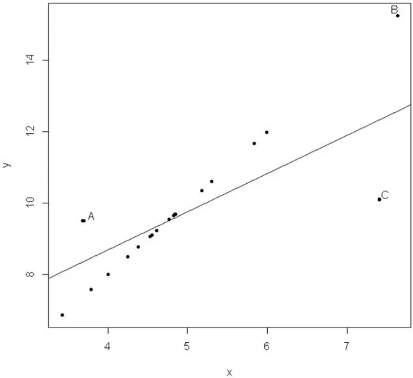
from the central tendency of the predictors. In a concise term a point (y′_i,x′_i) which does not follow the linear pattern of the bulk of the data but whose x′_iis not outlying is called vertical outlier. A point(y′_i,x′_i)whose correspondingx′_i is outlying is called a leverage point. A point (y′_i,x′_i)is a bad leverage point when it does not follow the pattern of the bulk of the data; otherwise, it is a good leverage point (this is because it

Figure 1.1: Scatter Plot Illustrating Outliers and Leverages

Figure 1.1 depicts the differences between outliers, good leverage points and bad

lever-age points. PointAis an outlier, pointBis a good leverage observation, and pointCis a bad leverage observation.

TheLSregression is extremely susceptible to influential observations. This is because an outlier may have a large residual which, when squared, it wrecks theLS objective function. This is illustrated in theLSregression fit of Figure 1.1 where pointsAandC

pulled theLSregression line from passing through pointBwhere the bulk of the data trend follows.

To summarize, theLSregression is susceptible to as little as one influential observation. As a consequence, parameter estimates and inferential statistics about the estimation

process turns out to be misleading. If LS regression is blindly implemented without any exploratory data analysis, it may be unknown when the analysis has severe flaws.

The phenomenon may lead to a conclusion that does not support the data in the actual

sense. It is therefore, necessary to make a right choice of regression methodology in

data analysis.

With the intent to curtail the drawbacks and risks of failure of Gaussian assumptions

in LS procedure, diagnostic approaches have been proposed for the identification of contaminated observations. These diagnostic tools are applicable in the framework of

robust regression as well.

1.7 Leverage and the Hat Matrix

By definition, the tendency for an observation to overwhelm an estimator relative to

its position in the predictor hyperplane, irrespective of whether the corresponding

re-sponse variable is an outlier or not is referred to as an observation’s leverage. The major

difference between conventional regression and robust regression lies in the

quantifi-cation of this concept.

To begin with, for a p-dimensional predictor variables in a regression model without intercept parameter, the Mahalanobis distance metric, di, for the ith observation is

given by

di=

√

wheremis the p×1 mean vector andCis the p×pcovariance matrix.

Furthermore, consider the scenario in which the intercept parameter is included in the

model, the ‘hat matrix’ replaces the Mahalanobis distances. This matrix (hat matrix) described as the p×p matrix H= X(X′X)−1X′, acquired the name hat matrix be-cause it maps the observed response variable into the predicted values of the response

variables as ˆy=X ˆβ =Hy. This matrix plays an important role in classical outlier diagnostics. Myers (2000) enumerated the properties of theHat matrixas follows:

1. The hat matrix is symmetric and idempotent.

2. The trace ofHequalsp, the dimensional size: i.e ∑n

i=1

hii=p.

3. Theith hat diagonalhii is bounded such that:

(a) For models with intercept, 1_n≤hii≤1,∀i,

(b) For models without intercept, 0≤hii≤1,∀i.

4. Ifhii =1, thenhi j=hji=0,∀i̸= j.

5. Every row ofH(and by symmetry, every column) sums to one i.e.

n ∑ j=1

hi j=1,∀i.

6. Theith hat diagonal,hii is monotonically related to theith Mahalanobis distance

disuch hii= d_i2 n−1+ 1 n. (1.5)

ten-dency in the predictor space (Myers, 2000). As a result, theLS-regression procedure uses the hat diagonal to measure its leverage. Since the sum of all n hat diagonals equals p, and thus 2p_n is twice the mean hat diagonal, Myers (2000) proposed a rule of thumb for identifying leverage points as any observation withhii ≥2p_n .

The main drawback of the hat diagonals and the Mahalanobis distance is that they are

both functions of the mean. As a result they are affected by the observation they are

supposed to identify. As can be seen from Equation (1.5), describing the relationship

of hat diagonal to the Mahalanobis distances, these hat diagonals are functions of the

classical mean denoted asm, and the corresponding sample covariance denoted asC. According to Billor et al. (2000), both m and C are susceptible to influential obser-vations, and hence, they are not reliable estimators. Consequently, the discussion of

more resistant estimator for m and C is hitherto a desirable alternative. Precisely, a robust Mahalanobis distance metric will be proposed by substitutingmandCby more resistant estimators of multivariate location and dispersion.

1.7.1 Altered Hat Matrix

The hat matrix is based on the predictor variables only. As a result, it does not account

for outlying observations in they-subspace. In order to account for the likely presence of outliers in the response variable, the n×n altered hat matrix, Hy is described as Hy=Xy(Xy′Xy)−1X′y. Myers (2000) reported that the altered hat matrix also have the

pfor the usual hat matrix. Myers (2000) has shown that

Hy=H+ rr′

SSE, (1.6)

whereris the residual vector andSSEthe sum of squares error, both computed from theLS-regression. SinceHyis based onH,LSresiduals andSSE, its diagonal elements are susceptible to outliers or high leverage points.

1.8 Outlier Diagnostics

In searching for outliers in the response variable, it is ideal to begin with residual

analysis. However, Myers (2000) stated that high leverage points tend to have small

residuals because they overwhelm the fitted values and are masked by it. Consequently,

a cautionary approach when making inferences from the set of residuals is ideal.

Given that residuals constitute the units of the response variable, the extent of what

constitutes a large residual is a function of the scale parameter. Hence, an estimate

forσ, denoted bySis used to re-scale the residuals. Myers (2000) suggested the root mean square error(RMSE)obtained from the classical regression analysis of variance

(ANOVA) table. The RMSE is then, defined in terms of an internally studentized residualgiven by

r′_i= ri

s√1−hii

. (1.7)

where ri is the ith element of the residual vector r. Lest for lack of independence,

Equation (1.7) follows a Studentt-distribution. Given that the numerator and denomi-nator are not independent andr_i′ does not follow a truet-distribution. However, Myers

(2000) deemed it to be nearlyt-like, and suggested that anith observation is deemed outlier if the corresponding|r_i′| ≥2.

The performance of a regression procedure can be assessed by viewing the regression

analysis when a particular observation is included and when it is removed and then

measure the change in both scenarios. This type of assessment is called ‘single point

deletion analysis’ or the ‘prediction residual(PRESS)approach’. For purpose of no-tation, ‘−i’ subscript could mean that the analysis is carried out without the ith data point. Therefore, ˆyi,−idenotes the fitted value atx′i when the regression is carried out

withoutx′_iandyi. Ordinarily, thePRESSanalysis appears to involve the computation

ofnseparate regressions, each with a reduced sample sizen−1. As a result of manip-ulations, only the full data regression is required. That is, the residualri,−i=yi−yˆi,−i

usually referred to as thePRESSresidual can be computed asri,−i=₍₁₋ri_h

ii).

The presence of outlier in the response space tends to inflate the estimate of scale,

s2 . To deflate such inflation, an alternative to the internally studentized residual is desirable. Myers (2000) suggested to compute,s2_−i, in thePRESSprocedure, where

s₋i=

√

(n−p)s2−_r2

i/(1−hii)

n−p−1 (1.8)

is used to compute theexternally studentized residualsdefined as

Rstudenti= yi−yˆi s₋i √ 1−hii . (1.9)

numerator and denominator are now independent. An outlier is identified by a Rstudent

value if|Rstudenti|>t(1−α),(n−p−1). When the effect of theith data point is high, the data point will have a larger Rstudent value than the internally studentized residual.

This is because the estimate of scale s2_−i used in the denominator without this data point tends to be smaller than the estimate of scale obtained when using all of the data.

1.9 Influence Diagnostics

Huber (1981) defines the term influence, as the relative effect of a particular observa-tion’s presence on the resulting estimator. Since high leverage outlier has a distorting

effect on theLSestimator, their deletion has a significant effect on the estimator. There-fore, they are said to be substantially influential. Armed with this definition, one can

infer that single point deletion analysis plays a significant role in influence diagnostics.

The influence of the ith observation can be measured using the statistic referred to as ‘difference in fits’ (DFFITS)-statistic, given as

DFFIT Si= ˆ yi−yˆi,−i s₋i √ hii . (1.10)

Myers (2000) have shown that theDFFIT S-statistic can be written as

DFFIT Si=Rstudenti[

hii

1−hii

]12 _(1.11)

The advantage of theDFFIT S-statistic as an influential diagnostic tool is that it con-stitutes an outlier diagnostic component,Rstudenti, and a leverage diagnostic

compo-nent, [ hii (1−hii)]

1

the outliers and leverages in its evaluation of an observation’s influence on an

estima-tor (Atkinson et al., 2004). For this reason, theDFFIT S-statistic is used as a measure to determine the influence of an outlier cluster on the proposed multiple regression

model.

More robust outlier identification, location and dispersion estimator as well as

outlier-resistant regression methodologies are now discussed in Chapter 2. These estimators

are resistant to contaminations of various sorts and can work well in data analysis when

CHAPTER 2

LITERATURE REVIEW

2.1 Introduction

This chapter discusses the various robust procedures for computing location and

dis-persion estimators and outlier identification procedures. In what follows is the review

of robust regression methods with emphasis on low breakdown and high breakdown

scenarios for multiple regression. A review of existing robust alternatives toLS multi-variate regression concludes this chapter.

Traditionally, nearly all robust outlier identification procedures are based on the

loca-tion and dispersion estimators. This accounts for why the two (localoca-tion and dispersion

estimator and outlier identification methods) are jointly discussed. Outlier

identifica-tion methods can be broadly classified into two groups, namely, the forward search

algorithms and the elemental or resampling set algorithms. The forward search

proce-dure heuristically searches for a ‘half subset’ from a data set through a forward stepping

algorithm. The method involves selecting an initial subset that is outlier-free and then

load it (initial subset) according to a decision criterion until the initial subset contains

‘half subset’. Observations with indexes corresponding to the half subset is used to

compute the robust location and dispersion. The robust location and dispersion

esti-mators are in turn, used to compute the Mahalanobis distance. Observations whose

as an outlier. The coordinatewise median, the Stahel-Donoho estimator, the Stalactite

plot analysis, the Orthogonalized Gnanadesikan-Kettenring estimator (OGK) and the block adaptive computationally efficient outlier nominator(BACON)are examples of the forward search algorithm procedure. The elemental or resampling set procedures

on the other hand computes the location and dispersion estimators by taking a subset

from a data set based on a given objective function that minimizes the error in the

subset selection criterion. A resampling step then optimizes this criterion by

lower-ing the objective function at each resampllower-ing step until an optimum subset which is

free is obtained. A location and dispersion estimator arising from this

outlier-free subset is then used to compute a Mahalanobis distance. A candidate outlier is that

observation whose index corresponds to the Mahalanobis distance that is greater than a

specified threshold (sayδ). The minimum volume ellipsoid(MV E), the minimum co-variance determinant(MCD)and the Deterministic minimum covariance determinant

(DetMCD)are members of robust outlier identification that implement the elemental or resampling procedure.

The goal of robust statistics in outlier identification is the desire to obtain a robust

multivariate location estimator, denoted bym, and a multivariate dispersion estimator, also denoted as C in such a way that the influence of spurious observations can be subdued. The significance of these techniques to robust regression arena hinges on the

ability to extract information about outlier presence as well as its structures especially

in multivariate settings. This implies a transformation from the Gaussian approach

of ‘equal weight assignment’ into another optimistic more robust approach of weight

p+1)/2]-observations in outlier identification as well as multiple regression settings. It is modified as h = [(n+k+1)/2];k= p+q in multivariate regression settings. The outlier identification procedures based on the location and dispersion estimators

discussed below is relative to the data matrixZy.

2.2 Location and Dispersion Estimators

Suppose that Zy is taken from a population with a multivariate normal distribution,

then the classical mean and covariance estimators are computed, respectively, as the

k×1 sample mean vector,

m= n ∑ i=1 zy,i n (2.1)

and thek×ksample covariance (dispersion) matrix,

C= n ∑ i=1 (zy,i−m)(zy,i−m)′ n−1 (2.2)

Equations (2.1) and (2.2) are apparently, functions of the mean and hence, any outlier

observation can erratically deflate or inflate them. The repercussions are that

infer-ences drawn from these estimators, such as the hat diagonals, for instance, are severely

unreliable in the presence of unusual or extreme observations. Therefore, it is

imper-ative to think of alternimper-ative estimators that can resist the influence of these extreme

observations.

One simple way to estimate m and Cis to adopt a robust multivariate location esti-mator in a coordinatewise manner. In the same way as the univariate location

estima-tion, replace the sample mean by the sample median for each of thek-variables. The covariance matrix turns out to be the covariance estimation that is centered by this

co-ordinatewise median. According to Billor et al. (2000), the coco-ordinatewise median is

thought to be more robust as much as 50% than the mean. Although the

coordinate-wise median and the dispersion estimator computed from it is robust, computational

convenience appears to have determined the choice of the median in the past. This is

because in the multivariate setting, the coordinatewise median location estimator is not

affine equivariant. According to Rousseeuw and Leroy (2003), this estimator is not

affine equivariant, implying that linear transformations of the data are not equivalently

transformed by the estimator. The procedures discussed below combine outlier

identi-fication with estimation of location and dispersion estimators. They are classified into:

the forward search procedures and elemental or resampling procedures.

2.2.1 The Forward Search Procedures

Several estimators exist that can replace the non robust sample mean vector and

dis-persion matrix estimators. Some of these estimators differ mainly in terms of their

objective functions and theoretical properties. The following are major outlier

resis-tant estimators for multivariate location and dispersion that adopt the forward search

procedure.

2.2.1(a) The Stahel-Donoho Estimator

Proposed independently by Stahel (1981), Donoho (1982) and Dodge (2002) described

es-ferently from the bulk of the data when they are outlying in a correct metrics. The

procedure is implemented in two stages. A projection computation is used to

deter-mine a robust distance in the first stage. At the second stage, the robust distances serve

as a weight function with a weighted mean vector and weighted dispersion matrix.

According to Rousseeuw and Leroy (1987), this approach is affine equivariant, and

at-tains high breakdown point when the data are in general position. The algorithm itself

is presented below.

Algorithm 2.1: The Stahel-Donoho Projection-based Location and Dispersion Al-gorithm;Source: Rousseeuw and Leroy (1987)

1. Obtain a robust distance, denoted byui, for theith observationzy,i, as:

ui= sup ||v||=1 |z′_y,iv−m ∀jed(z ′ y,jv)| m ∀ked|z ′ y,kv−_∀m_jed(z ′ y,jv)| , (2.3)

where v is the k×1 directional vector, through which the projections of all n

observations are made. The robust distance that is a function of weights obtained

from ui is used to classify outliers into a different cluster while the clean data

points remain in the main cluster.

2. Using thenrobust distances,uiand the data setZythe robust location estimator

is computed as m= n ∑ i=1 w(ui)zy,i n ∑ i=1 w(ui) , (2.4)