Classification on Open Ended Data Sets
Thomas Mensink, Jakob Verbeek, Florent Perronnin, Gabriela Csurka
To cite this version:
Thomas Mensink, Jakob Verbeek, Florent Perronnin, Gabriela Csurka. Large Scale Metric
Learning for Distance-Based Image Classification on Open Ended Data Sets. Farinella,
Gio-vanni Maria and Battiato, Sebastiano and Cipolla, Roberto. Advanced Topics in Computer
Vision, Springer, pp.243-276, 2013, 978-1-4471-5519-5.
<
10.1007/978-1-4471-5520-1 9
>
.
<
hal-00949416
>
HAL Id: hal-00949416
https://hal.inria.fr/hal-00949416
Submitted on 19 Feb 2014
HAL
is a multi-disciplinary open access
archive for the deposit and dissemination of
sci-entific research documents, whether they are
pub-lished or not.
The documents may come from
teaching and research institutions in France or
abroad, or from public or private research centers.
L’archive ouverte pluridisciplinaire
HAL
, est
destin´
ee au d´
epˆ
ot et `
a la diffusion de documents
scientifiques de niveau recherche, publi´
es ou non,
´
emanant des ´
etablissements d’enseignement et de
recherche fran¸
cais ou ´
etrangers, des laboratoires
publics ou priv´
es.
Image Classification on Open Ended Data Sets
Thomas Mensink, Jakob Verbeek, Florent Perronnin, and Gabriela Csurka
AbstractMany real-life large-scale datasets are open-ended and dynamic: new im-ages are continuously added to existing classes, new classes appear over time, and the semantics of existing classes might evolve too. Therefore, we study large-scale image classification methods that can incorporate new classes and training images continuously over time at negligible cost. To this end we consider two distance-based classifiers, the k-nearest neighbor (k-NN) and nearest class mean (NCM) clas-sifiers. Since the performance of distance-based classifiers heavily depends on the used distance function, we cast the problem into one of learning a low-rank metric, which is shared across all classes. For the NCM classifier we introduce a new met-ric learning approach, and we also introduce an extension to allow for met-richer class representations.
Experiments on the ImageNet 2010 challenge dataset, which contains over one million training images of thousand classes, show that, surprisingly, the NCM clas-sifier compares favorably to the more flexible k-NN clasclas-sifier. Moreover, the NCM performance is comparable to that of linear SVMs which obtain current state-of-the-art performance. Experimentally we study the generalization performance to classes that were not used to learn the metrics. Using a metric learned on 1,000 classes, we show results for the ImageNet-10K dataset which contains 10,000 classes, and ob-tain performance that is competitive with the current state-of-the-art, while being orders of magnitude faster.
Keywords Metric Learning, k-Nearest Neighbors Classification, Nearest Class Mean Classification, Large Scale Image Classification, Transfer Learning, Zero-Shot Learning, Image Retrieval
Thomas Mensink and Jakob Verbeek
LEAR Team - INRIA Grenoble, 655 Avenue de l’Europe, 38330 Montbonnot, France e-mail:[email protected]
Florent Perronnin and Gabriela Csurka
Xerox Research Centre Europe, 6 chemin de Maupertuis, 38240 Meylan, France e-mail:[email protected]
This chapter is largely based on previously published work [30,31].
1 Introduction
In the last decade we have witnessed an explosion in the amount of images and videos that are digitally available,e.g. in broadcasting archives or social media shar-ing websites. Scalable automated methods are needed to handle this huge volume of data, for retrieval, annotation and visualization purposes. This need has been rec-ognized in the computer vision research community and large-scale methods have become an active topic of research in recent years. The introduction of the Ima-geNet dataset [10], which contains more than 14M manually labeled images of 22K classes, has provided an important benchmark for large-scale image classification and annotation algorithms.
In this chapter we focus on the problem of large-scale, multi-class image classifi-cation, where the goal is to assign automatically an image to one class out of a finite set of alternatives,e.g. the name of main object appearing in the image, or a general label like the scene type of the image. The predominant approach to this problem is to treat it as a classification problem. To ensure scalability, often linear classifiers such as linear SVMs are used [39,27]. Additionally, to speed-up classification, di-mension reduction techniques could be used [46], or a hierarchy of classifiers could be learned [2,12]. Recently, impressive results have been reported on 10,000 or more classes [9,46,39]. For all these methods hold that they are trained by using stochastic gradient descend (SGD) algorithms, which access only a small fraction of the training data at each iteration [3].
Many real-life large-scale datasets are open-ended and dynamic: new images are continuously added to existing classes, new classes appear over time, and the se-mantics of existing classes might evolve too. At first glance, one-vs-rest classifiers (such as SVMs) trained with SGD algorithms appear to be the perfect solution. In-deed, classes can be trained independently, thus enabling to easily add new classes. Also since SGD algorithms are online algorithms they can accommodate for new samples easily. However, in order to apply these algorithms successfully we need to address several challenging problems. First, it is unclear to which classifier a new training sample should be fed; surely the sample should be used for the corre-sponding class, however feeding it as a negative sample to all other classes is not only costly but also suboptimal [35]. Second, for state-of-the-art performance the parameters of the SVM (such as the regularizer and the balance between positive and negative samples) are set by cross validation. The optimal value of these param-eters depend, among others, on the number of training samples and classes, and it is unclear how these should be adapted when applied on open ended datasets to allow for an increasing number of samples and classes over time. Therefore, we believe that standard one-vs-rest SVM classifiers are unsuitable for this task.
In this work, as an alternative, we explore distance-based classifiers which en-able the addition of new classes and new images to existing classes at (near) zero cost. These methods can be used continuously as new data becomes available, and additionally alternated from time to time with a computationally heavier method to learn a good metric using all available training data. In particular we consider two distance-based classifiers.
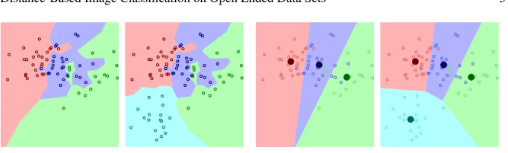
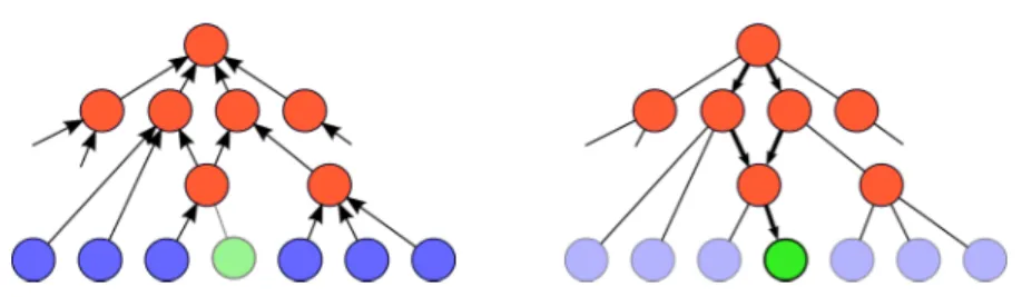
(a) K-NN Classification (b) NCM Classification
Fig. 1: Illustration of the classification rules of k-NN (a) and NCM (b). We also illustrate the effect of adding data from a new class to the data set.
The first is the k-nearest neighbor (k-NN) classifier, which uses all examples to represent a class, and is a highly non-linear classifier that has shown competitive performance for image classification [9,46,18]. New images (of new classes) are simply added to the database, and can be used for classification without further processing, see Figure1afor an illustration.
The second is the nearest class mean classifier (NCM), which represents classes by their mean feature vector of its elements, seee.g. [42]. Contrary to the k-NN classifier, this is an efficient linear classifier. To incorporate new images (of new classes), the relevant class means have to be adjusted or added to the set of class means, see Figure1bfor an illustration. In Section3, we introduce an extension which uses several prototypes per class, allowing a trade-off between the model complexity and the computational cost of classification.
The success of these methods critically depends on the used distance functions. Therefore, we cast our classifier learning problem as one of learning a low-rank Mahalanobis distance which is shared across all classes. The dimensionality of the low-rank matrix is used as regularizer, and to improve computational and storage ef-ficiency. In this chapter we explore several strategies for learning such a metric. For the NCM classifier, we propose a novel metric learning algorithm based on multi-class logistic discrimination (NCMML), where a sample from a multi-class is enforced to be closer to its class mean than to any other class mean in the projected space. We show qualitatively and quantitatively the advantages of our NCMML approach over the classical Fisher Discriminant Analysis [42]. For k-NN classification, we rely on the Large Margin Nearest Neighbor (LMNN) framework [44] and investigate two variations similar to the ideas presented in [44,6] that significantly improve classi-fication performance.
Most of our experiments are conducted on the ImageNet Large Scale Visual Recognition Challenge 2010 (ILSVRC’10) dataset, which consists of 1.2M training images of 1,000 classes. To apply the proposed metric learning techniques on such a large-scale dataset, we employ stochastic gradient descend (SGD) algorithms, which access only a small fraction of the training data at each iteration [3]. To allow metric learning on high-dimensional image features of datasets that are too large to fit in memory, we use in addition product quantization [17], a data compression technique
that was recently used with success for large-scale image retrieval [21] and classifier training [39]. As a baseline approach, we use the state-of-the-art approach of [39], which was also the winning entry in the 2011 edition of the challenge: Fisher vector image representations [36] are used to describe images and one-vs-rest linear SVM classifiers are learned independently for each class.
Surprisingly, we find that the NCM classifier outperforms the more flexible k-NN classifier, after learning a low-rank metric on the Fisher vector image repre-sentations. Moreover, the NCM classifier performs on par with the SVM baseline, and results are improved when we use the extension to allow for multiple centroids per class. Further we consider, among others, the generalization performance to new classes on the ImageNet-10K dataset (which consist of 4.5M training images of 10K classes) [9], a zero-shot setting where we estimate the mean of novel classes based on related classes in the ImageNet hierarchy, and image retrieval where we use a metric learned with our NCM classifier on the ILSVRC’10 dataset, to retrieve the most similar images for a given query on the INRIA Holidays [20] or the University of Kentucky Benchmark dataset (UKB) [32].
The rest of the chapter is organized as follows. In Section2we discuss a selec-tion of related work which is most relevant to this chapter. In Secselec-tion3we introduce the NCM classifier and the NCMML metric learning approach, together with an ex-tension to use multiple centroids (NCMC). In Section4we review LMNN metric learning for k-NN classifiers, and present two variants. We present extensive experi-mental results in Section5, analyzing different aspects of the proposed methods and comparing them to the current state-of-the-art in different application settings such as large scale image annotation, transfer learning and image retrieval. Finally, we present our conclusions in Section6.
2 Related work
In this section we review related work on large-scale image classification, metric learning, and transfer learning.
2.1 Large-scale image classification
The ImageNet dataset [10] has been a catalyst for research on large-scale image annotation. The current state-of-the-art [39,27] uses efficient linear SVM classi-fiers trained in a one-vs-rest manner in combination with high-dimensional bag-of-words [8,47] or Fisher vector representations [36]. Besides one-vs-rest training, large-scale ranking-based formulations have also been explored in [46]. Interest-ingly, their WSABIE approach performs joint classifier learning and dimensionality reduction of the image features. Operating in a lower-dimensional space acts as a regularization during learning, and also reduces the cost of classifier evaluation at
test time. Our proposed NCM approach also learns low-dimensional projection ma-trices but the weight vectors are constrained to be the projected class means. This allows for efficient addition of novel classes.
In [9,46] k-NN classifiers were found to be competitive with linear SVM clas-sifiers in a very large-scale setting involving 10,000 or more classes. The drawback of k-NN classifiers, however, is that they are expensive in storage and computa-tion, since in principle all training data needs to be kept in memory and accessed to classify new images. The storage issue is also encountered when SVM classifiers are trained since all training data needs to be processed in multiple passes. Product quantization (PQ) was introduced in [21] as a lossy compression mechanism for local SIFT descriptors in a bag-of-features image retrieval system. It has been sub-sequently used to compress bag-of-words and Fisher vector image representations in the context of image retrieval [22] and classifier training [39]. We also exploit PQ encoding in our work to compress high-dimensional image signatures when learning our metrics.
2.2 Metric learning
There is a large body of literature on metric learning, but in this section we limit ourselves to highlight just several methods that learn metrics for (image) classifi-cation problems. Other methods aim at learning metrics for verificlassifi-cation problems and essentially learn binary classifiers that threshold the learned distance to decide whether two images belong to the same class or not, seee.g. [33,19,23]. Yet an-other line of work concerns metric learning for ranking problems, i.e. to learn a metric between a query and the documents in the database, for example to address text retrieval tasks as in [1].
Among those methods that learn metrics for classification, the Large Margin Nearest Neighbor (LMNN) approach of [43,44] is specifically designed to sup-port k-NN classification. It tries to ensure that for each image a predefined set of target neighbors from the same class are closer than samples from other classes. Since the cost function is defined over triplets of points —that can be sampled in an SGD training procedure— this method can scale to large datasets. The set of target neighbors is chosen and fixed using theℓ2metric in the original space; this can be problematic as theℓ2distance might be quite different from the optimal metric for image classification. Therefore, we explore two variants of LMNN that avoid using such a pre-defined set of target neighbors, similar to the ideas presented in [6,44], both variants leading to significant improvements.
The large margin nearest local mean classifier [5] assigns a test image to a class based on the distance to the mean of its nearest neighbors in each class. This method was reported to outperform LMNN but requires computing all pairwise distances between training instances and therefore does not scale well to large datasets.
The TagProp method of [18] is a probabilistic nearest neighbor classifier; it con-sists in assigning weights to training samples based on their distance to the test
in-stance and in computing the class prediction by the total weight of samples of each class in a neighborhood. However, similar as [5], for training also TagProp requires pairwise distances between all training examples. Other closely related methods are metric learning by collapsing classes [14] and neighborhood component analy-sis [15]. As TagProp, for each data point these define weights to other data points proportional to the exponent of negative distance. In [14] the target is to learn a distance that makes the weights uniform for samples of the same class and close to zero for other samples. While in [15] the target is only to ensure that zero weight is assigned to samples from other classes. These methods also require computing distances between all pairs of data points, and therefore we do not consider any of these methods in our experiments.
Closely related to our NCMML metric learning approach for the NCM classi-fier is the LESS model of [41]. They learn a diagonal scaling matrix to modify theℓ2distance by rescaling the data dimensions, and include anℓ1penalty on the weights to perform feature selection. However, in their case, NCM is used to ad-dress small sample size problems in binary classification,i.e. cases where there are fewer training points (tens to hundreds) than features (thousands). Our approach differs significantly in that (i) we work in a multi-class setting and (ii) we learn a low-dimensional projection which allows efficiency in large-scale.
Another closely related method is the Taxonomy-embedding method of [45], where a nearest prototype classifier is used in combination with a hierarchical cost function. Documents are embedded in a lower dimensional space in which each class is represented by a single prototype. In contrast to our approach, they use a predefined embedding of the images and learn low-dimensional classifies, and therefore their method resembles more to the WSABIE method of [46].
The centroid-based classification method explored in [48] is also related to our method. It uses a NCM classifier and anℓ2distance in a subspace that is orthog-onal to the subspace with maximum within-class variance. To obtain the optimal subspace, it computes the first eigenvectors of the within-class covariance matrix, which has a computational cost betweenO(D2)andO(D3), this is undesirable for high-dimensional feature vectors. Moreover, this metric is heuristically obtained, rather than directly optimized for maximum classification performance.
2.3 Transfer learning
The term transfer learning is used to refer to methods that share information across classes during learning. Examples of transfer learning in computer vision include the use of part-based or attribute class representations. Part-based object recognition models [11] define an object as a spatial constellation of parts, and share the part de-tectors across different classes. Attribute-based models [24] characterize a category (e.g. a certain animal) by a combination of attributes (e.g. is yellow, has stripes, is carnivore), and share the attribute classifiers across classes. Other approaches in-clude biasing the weight vector learned for a new class towards the weight vectors
of classes that have already been trained [40]. Zero-shot learning [25] is an extreme case of transfer learning where for a new class no training instances are available but a description is provided in terms of parts, attributes, or other relations to already learned classes. Transfer learning is related to multi-task learning, where the goal is to leverage the commonalities between several distinct but related classification problems, or classifiers learned for one type of images (e.g. ImageNet) are adapted to a new domain (e.g. imagery obtained from a robot camera), seee.g. [38,34].
In [37] various transfer learning methods were evaluated in a large-scale setting using the ILSVRC’10 dataset. They found transfer learning methods to have little added value when training images are available for all classes. In contrast, transfer learning was found to be effective in a zero-shot learning setting, where classifiers were trained for 800 classes, and performance was tested in a 200-way classification across the held-out classes.
In this chapter we also aim at transfer learning, in the sense that we allow only a trivial amount of processing on the data of new classes (storing in a database, or averaging), and rely on a metric that was trained on other classes to recognize the new ones. In contrast to most works on transfer learning, we do not use any intermediate representation in terms of parts or attributes, nor do we train classifiers for the new classes. While also considering zero-shot learning, we further evaluate performance when combining a zero-shot model inspired by [37] with progressively more training images per class, from one up to thousands. We find that the zero-shot model provides an effective prior when a small amount of training data is available.
3 The nearest class mean classifier
The nearest class mean (NCM) classifier assigns an image to the classc∗∈ {1, . . . ,C}
with the closest mean:
c∗= argmin c∈{1,...,C} d(xxx,µµµc), (1) µ µ µc= 1 Nci:
∑
yi=c xxxi, (2)whered(xxx,µµµc)is the Euclidean distance between an imagexxxand the class mean
µ µ
µc, andyi is the ground-truth label of imagei, andNc is the number of training
images for classc. The NCM classifier is a linear classifier, which allows for efficient evaluation at test time, see Figure1bfor an illustration.
Next, we introduce our NCM metric learning approach, and its relations to exist-ing models. Then, we present an extension to use multiple centroids per class, which transforms the NCM into a non-linear classifier. Finally, we explore some variants of the objective which allow for smaller SGD batch sizes, and we give some insights in the critical points of the objective function.
3.1 Metric learning for the NCM classifier
In this section we introduce our metric learning approach, which learns a metric by maximizing the log-likelihood of correct classification. We will refer to our method as “nearest class mean metric learning” (NCMML). In our method we replace the Euclidean distance in NCM, Eq. (1), by a learned (squared) Mahalanobis distance:
dM(xxx,xxx′) = (xxx−xxx′)⊤M(xxx−xxx′), (3)
wherexxxandxxx′ areDdimensional vectors, andM is a positive definite matrix. We focus on low-rank metrics withM=W⊤W andW ∈IRd×D, whered≤Dacts as regularizer and improves efficiency for computation and storage. The Mahalanobis distance induced byW is equivalent to the squaredℓ2distance after linear projection of the feature vectors on the rows ofW:
dW(xxx,xxx′) = (xxx−xxx′)⊤W⊤W(xxx−xxx′)
=kW xxx−W xxx′k22. (4) In this chapter, we do not consider using the more general formulation ofM=
W⊤W+S, whereSis a diagonal matrix, as in [1]. While this formulation requires onlyDadditional parameters to estimate, it still requires computing distances in the original high-dimensional space. This is costly for the dense and high-dimensional (4K-64K) Fisher vectors representations we use, as detailed in Section5.
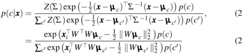
We formulate the NCM classifier using a probabilistic model based on multi-class logistic regression and define the probability for a multi-classcgiven a feature vector xxxas: p(c|xxx) = exp − 1 2dW(xxx,µµµc) ∑Cc′=1exp −12dW(xxx,µµµc′) . (5)
This definition may also be interpreted as giving the posterior probabilities of a generative model, wherep(xxx|c) =N (xxx;µµµc,Σ), is a Gaussian with meanµµµc, and a covariance matrixΣ= W⊤W−1
, which is shared across all classes1. Using Bayes rule we obtain: p(c|xxx) = p(xxx|c)p(c) p(xxx) = N (xxxi;µµµ c,Σ)p(c) ∑c′N (xxxi;µµµc′,Σ)p(c′) , (6) = Z(Σ)exp − 1 2(xxx−µµµc)⊤Σ−1(xxx−µµµc) p(c) ∑c′Z(Σ)exp −12(xxx−µµµc′)⊤Σ−1(xxx−µµµc′)p(c′) , (7) = exp − 1 2dW(xxx,µµµc) ∑Cc′=1exp −12dW(xxx,µµµc′) , (8)
1 Strictly speaking the covariance matrix is not properly defined as the low-rank matrixW⊤Wis
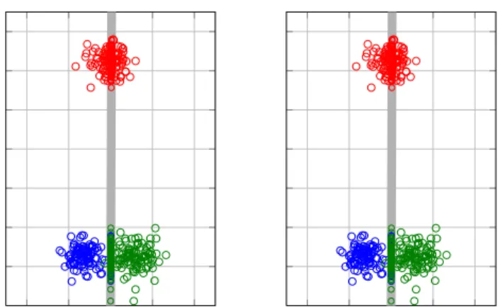
Fig. 2: Illustration to compare FDA (left) and NCMML (right), the obtained projec-tion direcprojec-tion is indicated by the gray line on which also the projected samples are plotted. For FDA the result is clearly suboptimal since the blue and green classes are collapsed in the projected space. While the proposed NCMML method finds a projection which separates the classes reasonably well.
where the class probabilities p(c)are set to be uniform over all classes. Later, in Eq. (27), we formulate an NCM classifier with non-uniform class probabilities.
We learn the projection matrixWin a discriminative manner, by maximizing the log-likelihood of the correct predictions of the training images:
L = 1 N N
∑
i=1 lnp(yi|xxxi). (9)The gradient of the NCMML objective Eq. (9) is:
∇WL = 1 N N
∑
i=1 C∑
c=1 αicW zzziczzz⊤ic, (10)whereαic=p(c|xxxi)−[[yi=c]],zzzic=µµµc−xxxi, and we use the Iverson brackets[[·]]
that equals one if its argument is true and zero otherwise.
Although not included above for clarity, the terms in the log-likelihood in Eq. (9) could be weighted in cases where the class distributions in the training data are not representative for those when the learned model is applied.
3.2 Relation to existing linear classifiers
In this section we related the NCM classifier and the proposed NCMML approach to other linear models.
First we compare the NCMML objective with the classical Fisher Discriminant Analysis (FDA). The objective of FDA is to find a projection matrixW that maxi-mizes the ratio of between-class variance to within-class variance:
LFDA=tr W S BW⊤ W SWW⊤ , (11)
whereSB=∑Cc=1NNc(µµµ−µµµc)(µµµ−µµµc)⊤ is the weighted covariance matrix of the
class centers (andµµµis the data center), andSW=∑Cc=1NNcΣcis the weighted sum of
within class covariance matricesΣc. Also to obtain a well-defined problem,W has
a constraint on the norms of its columns. Seee.g. [42] for more details on the FDA. In the case where the within class covariance for each class equals the identity matrix, the FDA objective seeks the direction of maximum variance in SB. This
equals to a PCA projection on the class means, which has the objective to maximize tr W⊤SBW
, also with a constraint on the norms ofW. The result of using the unsupervised PCA technique, is that it ignores the class information in the projected space, it just maximizes the variance between all class means. To illustrate this, we show an example of a two-dimensional problem with three classes in Figure2. In contrast to FDA, our NCMML method only aims at separating class means which are nearby in the projected space, so as to ensure correct predictions. The resulting projection direction separates the three classes reasonably well.
To relate the NCM classifier to other linear classifiers, we represent them with the class specific score function:
f(c,xxx) =www⊤cxxx+bc, (12)
that assigns a sample xxxto the class with maximum score. NCM can be seen as a linear classifier by defining fNCMwith bias and weight vectors given by:
bc=−12kWµµµck22, (13) wwwc=W⊤Wµµµc. (14)
This is proportional to the Mahalanobis distance up to an additive constant that is constant with respect to the classc, and therefore irrelevant for classification.
These definitions allows us relating the NCM classifier to other linear methods. For example, we obtain standard multi-class logistic regression, if the restrictions onbcandwwwcare removed. Note that these are precisely the restrictions that allows
us adding new classes at near-zero cost, since the class specific parametersbcand w
wwcare defined by just the class meansµµµcand the class-independent projectionW.
In the WSABIE method [46], the classifier fWSABIE, is defined usingbc=0 and, w
w
wc=W⊤vvvc (15)
whereW ∈IRd×D is also a low-rank projection matrix shared between all classes, andvvvcis a class specific weight vector of dimensionalityd, both learned from data.
This is similar to NCM if we setvvvc=Wµµµc. As in multiclass logistic regression,
however, for WSABIE thevvvcneed to be learned from scratch for new classes.
The NCM classifier can also be related to the solution of ridge-regression (RR, or regularized linear least-squares regression), which also uses a linear score function. The parametersbcandwwwcare learned by optimizing the squared loss:
LRR= 1 N
∑
i fRR(c,xxxi)−yic 2 +λkwwwck22, (16)whereλ acts as regularizer, and whereyic=1, if imageibelongs to classc, and yic=0 otherwise. The lossLRRcan be minimized in closed form and leads to:
bc= Nc N, (17) w w wc= Nc N µµµ ⊤ c(Σ+λI)−1, (18)
whereΣis the (class-independent) data covariance matrix,seee.g. [42]. Just like the NCM classifier, the RR classifier also allows to add new classes at low cost, since the class specific parameters can be found from the class means and counts once the data covariance matrix Σ has been estimated. Moreover, ifNc is equal for all
classes, RR is similar to NCM withW set such thatW⊤W = (Σ+λI)−1.
Finally, the Taxonomy-embedding method of [45], can be rewritten such that it equals the linear classifier fTAXusing:
bc=−12kvvvck22, (19) w
w
wc=W⊤W vvvc, (20)
where the class-specific weight vectorsvvvcare learned from the data andW ∈IRC×D
projects the data to aCdimensional space. The projection matrixW is set using a closed-form solution based on ridge-regression. This method relates to the WSABIE method since it also learns the classifier in low-dimensional space (ifC<D), how-ever in this case the projection matrixW is given in closed-form. It also shares the disadvantage of the WSABIE method: it cannot generalize to novel classes without retraining the low-dimensional class-specific vectorsvvvc.
3.3 Non-linear NCM with multiple class centroids
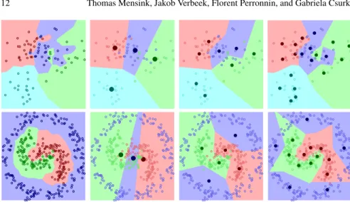
In this section we extend the NCM classifier to allow for more flexible class repre-sentations, which result in non-linear classification, see Figure3for an illustration. The idea is to represent each class by a set of centroids, instead of only the class mean. Assume that we have obtained a set ofkcentroids{mmmc j}k
j=1for each classc. We define the posterior probability for a centroidmmmc jas:
Fig. 3: Illustration of non-linear classification using multiple centroids on not lin-early separable data. From left to right we show, k-NN classification (k=1), NCM classification, and NCMC classification with 2 and 5 centroids respectively.
p(mmmc j|xxx) = 1 Zexp − 1 2dW(xxx,mmmc j) , (21) whereZ=∑c∑jexp −21dW(xxx,mmmc j)
is the normalizer. The posterior probability for classcis then given by:
p(c|xxx) =
k
∑
j=1p(mmmc j|xxx). (22)
This model also corresponds to a generative model, where the probability for a feature vectorxxx, to be generated by classc, is given by a Gaussian mixture distribu-tion: p(xxx|c) = k
∑
j=1 πc jN (xxxi;mmmc j,Σ), (23)with equal mixing weightsπc j=1/k, and the covariance matrixΣ shared among
all classes. We refer to this method as the nearest class multiple centroids (NCMC) classifier. A similar model was independently developed recently for image retrieval in [29]. Their objective, however, is to discriminate between different senses of a textual query, and they use a latent model to select the sense of a query.
To learn the projection matrixW, we again maximize the log-likelihood of cor-rect classification, for which the gradient w.r.t.W in this case is given by:
∇WL = 1
Ni
∑
,c,jαic jW zzzic jzzz⊤
wherezzzic j=mmmc j−xxxi, and
αic j=p(mmmc j|xxxi)−[[c=yi]]
p(mmmc j|xxxi) ∑j′p(mmmc j′|xxxi)
. (25)
To obtain the centroids of each class, we apply k-means clustering on the features xxxbelonging to that class, using theℓ2distance. The valuekoffers a transition be-tween NCM (k=1), and a weighted k-NN (kequals all images per class), where the weight of each neighbor is defined by the soft-min of its distance,c.f. Eq. (21). This is similar to TagProp [18], used for multi-label image annotation, which assigns a probability to a classcbased on the class labels and distances of the images in the training set: p(c|xxxi) =
∑
j πi j[[yj=c]], πi j= exp −1 2dW(xxxi,xxxj) ∑j′exp −1 2dW(xxxi,xxxj′) (26)In Figure3we illustrate the influence of increasingkon the obtained classification boundaries, and made the comparison with the k-NN (k=1) classifier.
Instead of using a fixed set of class means, it could be advantageous to iterate the k-means clustering and the learning of the projection matrixW. Such a strat-egy allows the set of class centroids to represent more precisely the distribution of the images in the projected space, and might further improve the classification per-formance. However the experimental validation of such a strategy falls beyond the scope of this paper.
3.4 Alternative objective for small SGD batches
Computing the gradients for NCMML in Eq. (10) and NCMC in Eq. (24) is rel-atively expensive, regardless of the number ofmsamples used per SGD iteration. The cost of this computation is dominated by the computation of the squared dis-tancesdW(xxx,µµµc), required to compute them×Cprobabilitiesp(c|xxx)forCclasses
in the SGD update. To compute these distances we have two options. First, we can compute them×Cdifference vectors(xxx−µµµc), project these on thed×Dmatrix W, and compute the norms of the projected difference vectors, at a total cost of O dD(mC) +mC(d+D)
. Second, we can first project both themdata vectors and Cclass centers, and then compute distances in the low dimensional space, at a total cost ofO dD(m+C) +mC(d)
. Note that the latter option has a lower complexity, but still requires projecting all class centers at a costO(dDC), which will be the dominating cost when using small SGD batches withm≪C. Therefore, in practice we are limited to using SGD batch sizes withm≈C=1,000 samples.
In order to accommodate for fast SGD updates based on smaller batch sizes, we replace the Euclidean distance in Eq. (5) by the dot-product plus a class specific bias sc. The probability for classcis now given by:
Distances inDdimensionsO dD(mC) +mC(d+D)
Distances inddimensions O dD(m+C) +mC(d)
Dot product formulation O dD(m) +mC(D)
Table 1: Comparison of complexity of the considered alternatives to compute the class probabilitiesp(c|xxx). p(c|xxxi) = 1 Zexp xxx⊤i W⊤Wµµµc+sc , (27)
whereZdenotes the normalizer. The objective is still to maximize the log-likelihood of Eq. (9). The efficiency gain stems from the fact that we can avoid projecting the class centers onW, by twice projecting the data vectors: ˆxxxi=xxx⊤iW⊤W, and then
computing dot-products in high dimensional spacehxxxˆi,µµµci. For a batch ofmimages,
the first step costs O(mDd), and the latterO(mCD), resulting in a complexity of O dD(m) +mC(D)
. This complexity scales linearly withm, and is lower for small batches withm≤d, since in that case it is more costly to project the class vectors onW than on the double-projected data vectors ˆxxxi. For clarity, we summarize the
complexity of the different alternatives we considered in Table1.
A potential disadvantage of this approach is that we need to determine the class-specific biasscwhen data of a new class becomes available, which would require
more training than just computing the data mean for the new class. However, we expect a strong correlation between the learned biasscand the biased based on the
norm of the projected meanbc. Similar as used for Eq. (5), we could interpret the
class probabilities in Eq. (27) as those being generated by a generative model where the class-conditional modelsp(xxx|c)are Gaussian with a shared covariance matrix. We continue from Eq. (7) and obtain:
p(c|xxx) = Z(Σ)exp − 1 2(xxx−µµµc)⊤Σ−1(xxx−µµµc) p(c) ∑c′Z(Σ)exp −12(xxx−µµµc′)⊤Σ−1(xxx−µµµc′)p(c′) , (28) = exp xxx ⊤ i W⊤Wµµµc−21kWµµµck22 p(c) ∑c′exp xxx⊤iW⊤Wµµµc′−21kWµµµc′k22p(c′) (29) In this interpretation, the class specific biasesscdefine class prior probabilities given
by p(c)∝exp 21kWµµµck2
2+sc. Therefore, a uniform prior is obtained by setting sc=−12kWµµµck22=bc. A uniform prior is reasonable for the ILSVRC’10 data, since
the classes are near uniform in the training and test data.
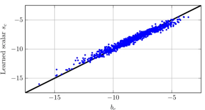
Experimentally we find that using this formulation yields comparable results as using the Euclidean distance. As expected we find a strong correlation between the learned biasscand the norm of the projected meanbc, shown in Figure4. Indeed, the
classification performance differs insignificantly if at evaluation time we setsc=bc
−15 −10 −5 −15 −10 −5 bc Le ar n e d s c al ar sc
Fig. 4: The learned class-specific biasesscand the norm of the projected meansbc
are strongly correlated.
Thus, even if we train the metric by using class-specific biases, we can use the learned metric in the NCM classifier with the bias based on the norm of the projected mean, which is easily computed for data of new classes.
3.5 Critical points of low rank metric learning
We use a low-rank Mahalanobis distance whereM=W⊤W, as a way to reduce the number of parameters and to gain in computational efficiency. Learning a full Ma-halanobis distance matrixM, however, has the advantage that the distance is linear inMand that the multi-class logistic regression objective of Eq. (9) is therefore con-cave inM[4, page 74]. Using a low-rank formulation, on the other hand, yields a distance which is quadratic in the parametersW, therefore the objective function is no longer concave. In this section we investigate the critical-points of the low-rank formulation by analyzingW when the optimization reaches a (local) minimum, and considering the gradient for the corresponding full matrixM=W⊤W.
The gradient of the objective of Eq. (9) w.r.t. toMis:
∇ML = 1
N
∑
i,cαiczzziczzz⊤
ic≡H, (30)
whereαic=p(c|xxxi)−[[yi=c]], andzzzic=µµµc−xxxi. Then Eq. (10) follows from the
matrix chain rule, and we re-define∇WL ≡2W H. From the gradient w.r.t.W we immediately observe thatW=0 leads to a degenerate case to obtain a zero gradient, and similarly for each row ofW. Below, we concentrate on the non-degenerate case. We observe thatHis a symmetric matrix, containing the difference of two posi-tive definite matrices. Further, we observe that whenH=0,i.e. when we reach the minimum of the full Mahalanobis distance, we obtain zero gradient forW. Here we analyzeHwhen the gradient w.r.t.W reaches a zero point. In the analysis below we
use the eigenvalue decomposition ofH=VΛV⊤, with the columns ofV being the eigenvectors, and the eigenvalues are on the diagonal ofΛ.
We can now express the gradient forW as
∇WL =2WVΛV⊤≡G. (31)
Thus the gradient of thei-th row ofW, which we denote bygggi, is a linear combi-nation of the eigenvectors ofH:
gggi≡
∑
jλjhwwwi,vvvjivvvj, (32)
wherewwwi andvvvj denote thei-th row ofW and the j-th column ofV respectively.
Thus an SGD gradient update will drive a row ofW towards the eigenvectors ofH that (i) have a large positive eigenvalue, and (ii) are most aligned with that row of W. This is intuitive, since we would expect the low-rank formulation to focus on the most significant directions of the full-rank metric.
Moreover, the expression for the gradient in Eq. (32) shows that at a critical pointW∗ of the objective function, all linear combination coefficients are zero:
∀i,j:λjhwww∗i,vvvji=0.This indicates that at the critical point, for each rowwww∗i and
each eigenvectorvvvjit holds that eitherwww∗i is orthogonal tovvvj, or thatvvvjhas a zero
associated eigenvalue,i.e.λj=0. Thus, at a critical pointW∗, the corresponding
gradient for the full rank formulation at that point, withM∗=W∗⊤W∗, is zero in the subspace spanned byW∗.
Given this analysis, we believe it is unlikely to attain poor local minima using the low rank formulation. Indeed, the gradient updates forW are aligned with the most important directions of the corresponding full-rank gradient, and at convergence the full-rank gradient is zero in the subspace spanned byW. To confirm this, we have also experimentally investigated this by training several times with different random initializations ofW. We observe that the classification performance differs at most
±.1% on any of the error measures used in Section5, and that the number of SGD iterations selected by the early stopping procedure are of the same order.
3.6 Transfer Learning with the Nearest Class Mean Classifier
In this section we describe how we can use the NCM classifier in a zero-shot setting. Inspired by [37], we propose to use the ImageNet hierarchy to estimate the mean of novel classes from the means of related training classes, see Figure 5 for an illustration. We follow ideas of [37] and estimate the mean of a novel classµµµzusing the means of its ancestor nodes in the ImageNet class hierarchy:µµµz= 1 |Az|
∑
a∈Az µ µ µa, (33)Fig. 5: Illustration of the estimation of the zero-shot prior on a mean. In the first step (left) the means of train classes (blue) are propagated upwards in the ImageNet hierarchy to the internal nodes (red). In the second step (right) the prior is estimated as the average of all the ancestor nodes of the new class (green).
whereAzdenotes the set of ancestors of nodez, andµµµais the mean of ancestora. The mean of an internal node,µµµa, is computed as the average of the means of all its descendant training classes. In our experiments, the classes of interest are always leaf-nodes of the hierarchy.
In the setting where we also have a few images of the new class, we can combine the zero-shot prior with the mean of the sample images. If we view the estimation of each class mean as the estimation of the mean of a Gaussian distribution, then the mean of a sample of imagesµµµscorresponds to the Maximum Likelihood (ML) esti-mate, while the zero-shot estimateµµµzcan be thought of as a prior. We can combine the prior with the ML estimate to obtain a maximum a-posteriori (MAP) estimate
µ µ
µpon the class mean. The MAP estimate of the mean of a Gaussian is obtained by:
µµµp=nµµµs+mµµµz
n+m , (34)
wheren is the number of images used to compute the ML estimate of the sample meanµµµs, and the prior obtains a weightmdetermined on the validation set [13].
4 K-NN Metric Learning
We compare the NCM classifier to the k-NN classifier, a frequently used distance based classifier. The k-NN classifier is attractive since it is very intuitive, just as-signing the class of the nearest neighbors to a test image, see Figure1afor an il-lustration. Just as for the NCM classifier, the k-NN classifier relies on distances, and thus it is essential to use a metric in which nearby images are also semantically related. In this section we discuss metric learning for k-NN classifiers, used to learn a low-rank Mahalanobis distanceM=W⊤W, whereW ∈IRd×D.
For successful k-NN classification, the majority of the nearest neighbors should be of the same class. This is reflected in the Large Margin Nearest Neighbors (LMNN) metric learning objective of [43,44]. LMNN is defined over triplets
con-sisting of a query imageq, a positive image pfrom the same class, and a negative imagenfrom another class. The objective is to get the distance betweenqand p smaller than the distance betweenqandn, using the hinge-loss to upper bound the zero/one loss:
Lqpn=1+dW(xxxq,xxxp)−dW(xxxq,xxxn)+, (35)
where[z]+=max(0,z)is the positive part ofz. The hinge-loss for a triplet is zero
if the negative imagenis at least one distance unit farther from the queryq than the positive imagep, and the loss is positive otherwise. The final learning objective sums the losses over all triplets:
LLMNN= N
∑
q=1∑
p∈Pq∑
n∈Nq Lqpn, (36)wherePqandNqdenote a predefined set of positive and negative images for each
query imageq. An important design choice is how to setPqandNqfor each query.
For the set of negative imagesNq, we follow [44] and use all images not belonging
to the class of the query image. Below, we describe several variants for the set of positive imagesPq.
Also in this case we can weight the terms in the loss function to account for non-representative class proportions in the training data.
4.1 Choice of target neighbors
For LMNN a set of targetPqfor a queryqis set to some images from the same class.
The rationale is that if we ensure that these targets are closer than the instances of the other classes, then the k-NN classification will succeed. To select the set of targets we consider three alternatives:
1. In the basic version of LMNN the set of targetsPqis set to the query’sknearest
neighbors from the same class, using theℓ2distance. Since this selection method tries to ensure that theℓ2-targets will also be the closest points using the learned metric, it implicitly assumes that theℓ2distance in the original space is a good similarity measure. In practice, however, this might not be the case.
2. The set of targets Pq is defined to contain all images of the same class asq,
hence the selection is independent on the metric. This is similar to [6] where the same type of loss was used to learn image similarity defined as the scalar product between feature vectors after a learned linear projection.
3. The set of targetsPqis dynamically updated to contain thekimages of the same
class that are closest toqusing the current metricW. Hence different target neigh-bors can be selected depending on the current metric. This method corresponds to minimizing the loss function also with respect to the choice ofPq. A
simi-lar approach has been proposed in [44], where everyT iterationsPqis redefined
using target neighbors according to the current metric.
A potential disadvantage of the the last method is that it requires frequent re-computation of the target neighbors. However, below we describe an efficient gra-dient evaluation method, which allows to approximate the dynamic set ofPqat each
iteration at a negligible additional cost compared to using a fixed set of target neigh-bors or using all images of the same class as targets.
Next, we will discuss an efficient triplet sampling and gradient evaluation algo-rithms to increase the efficiency of the SGD training.
4.2 Triplet sampling strategy.
Here, we describe a sampling strategy which obtains the maximal number of triplets frommimages selected per SGD iteration. Using a smallmis advantageous since the cost of the gradient evaluation is in large part determined by computing the projectionsW xxxof the images, and the cost of decompressing the PQ encoded sig-natures, if these are used.
To generate triplets we first select uniformly at random a classc, that will provide the query and positive images. WhenPqis set to contain all images of the same class,
we sampleρmimages from classc, with 0<ρ <1, and the remaining(m−ρm)
images are uniformly sampled from the other classes. We can consider the number of tripletstwe can generate as a function ofρfor a given ‘budget’ ofmimages to be accessed. In the case wherePqis set to contain all images from the same class,
the number of tripletstwe can generate for a specificρ is given by:
t(ρ) = (ρm)(ρm−1)(m−ρm), (37) since we can pair theρmimages with theρm−1 other images from the same class, and each pair forms a triplet with any of them−ρmnegative sampled images. The number of tripletstcan be approximated by:
t(ρ)≈m3ρ2(1−ρ), (38) and hence, the number of triplets is maximized when we chooseρ ≈2
3, in which case we can construct about 274m3triplets. In our experiments, we useρ =2
3 and m=300 images per iteration, leading to about 4 million triplets per iteration.
For other choices ofPqwe do the following:
• For a fixed set of target neighbors, we still sample13mnegative images, and take as many query images together with their target neighbors until we obtain 23m images allocated for the positive class.
• For a dynamic set of target neighbors we simply select the closest neighbors among the 23msampled positive images using the current metricW. Although
approximate, this avoids computing the dynamic target neighbors among all the images in the positive class.
An alternative to obtain roughly 4 million triplets is to sample two images from each of theC=1,000 classes. In this case, there are two query images per class, each forming a pair with the other positive image, and each pair can form a triplet with the 2(C−1)images of other classes, leading to 4C(C−1)≈4 million triplets. A potential advantage of this method is that the gradient is computed in each iteration from triplets generated using all possible combinations of classes, and therefore, the gradient might be more informative. However, this sampling strategy does not allow for fast approximation of the dynamic neighbors, and we would need to access m=2,000 images, which is about 7 times more costly than using the described approach withm=300.
4.3 Efficient gradient evaluation.
For either choice of the target setPq, the gradient can be computed without explicitly
iterating over all triplets. In this section we introduce an efficient gradient evaluation method, which uses sorting of the distances w.r.t. query images.
The sub-gradient of the loss of a triplet is given by:
∇WLqpn= [[Lqpn>0]]2W
xxxqpxxx⊤qp−xxxqnxxx⊤qn
, (39)
wherexxxqp=xxxq−xxxp, andxxxqn=xxxq−xxxn. By observing that the gradient takes the
form of outer products of the feature vectors, we can write the gradient w.r.t.Lq= ∑p,nLqpnin matrix form as:
∇WLq=2W X AX⊤, (40)
whereXcontains themfeature vectors used in an SGD iteration, andAis a coeffi-cient matrix. This shows that onceAis available, the gradient can be computed in timeO(m2), even if a much larger number of triplets is used.
WhenPq contains all images of the same class, the gradient per query can be
rewritten as: ∇WLq= +2W
∑
p∑
n [[Lqpn>0]] (xxxpxxx⊤p−xxxqxxx⊤p−xxxpxxx⊤q) −2W∑
n∑
p [[Lqpn>0]] (xxxnxxx⊤n−xxxqxxx⊤n−xxxnxxx⊤q). (41)Which shows that the coefficient matrix Acan be computed from the number of hinge-loss generating triplets in which each p∈Pqand eachn∈Nqfor a queryq
Algorithm 1Compute coefficientsAqnandAqp.
1. For positive images redefinedW(xxxq,xxxp)←dW(xxxq,xxxp) +1 to account for the margin.
2. Sort distances w.r.t.qin ascending order.
3. Cn(i)←∑ij=1[[j∈Nq]], the number of negative images up to each position.
4. Cp(i)←∑mj=i+1[[j∈Pq]], the number of positive images after each position.
5. Read-off the number of hinge-loss generating triplets of imageporn: Aqn=−2Cp(rnk(q,n)) Aqp=2Cn(rnk(q,p)),
where rnk(q,p)indicates the rank of documentpfor the queryq, and similar for rnk(q,n).
Aqn=2
∑
p [[Lqpn>0]], Apq=−2∑
n [[Lqpn>0]], (42) Aqq=∑
p Aqp−∑
n Aqn, App=∑
q Aqp, Ann=∑
q Aqn. (43)In Algorithm1we describe how to efficiently compute the coefficients, which sorts the distances w.r.t. the queryqand then can read of the number of hinge-loss generating triplets. The same algorithm can be applied when using a small set of fixed, or dynamic target neighbors. In particular, the sorted list allows to dynami-cally determine the target neighbors at a negligible additional cost. In this case only the selected target neighbors obtain non-zero coefficients, and we only accumulate the number of target neighbors after each position in step 3 of the algorithm.
The cost of this algorithm isO(mlogm)per query, and thusO(m2logm)when using O(m)query images per iteration. This is significantly faster than explicitly looping over allO(m3)triplets.
Note that while this algorithm enables fast computation of the sub-gradient of the loss, the value of the loss itself cannot be determined using this method. However, this is not a problem when using an SGD approach, as it only requires gradient evaluations, not function evaluations.
5 Experimental Evaluation
In this section we experimentally validate our models described in the previous sec-tions. We first describe the dataset and evaluation measures used in our experiments, followed by the presentation of the experimental results.
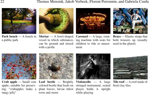
Park bench—A bench in a public park
Mortar—A bowl-shaped vessel in which substances can be ground and mixed with a pestle
Carousel—A large, rotat-ing machine with seats for children to ride or amuse-ment
Brace—Elastic straps that hold trousers up (usually used in the plural)
Crab apple—Small sour apple; suitable for preserv-ing; “crabapples make a tangy jelly”
Leaf beetle — Brightly colored beetle that feeds on plant leaves; larvae infest roots and stems
Violoncello — A large stringed instrument; seated player holds it upright while playing
Tile roof—A roof made of fired clay tiles
Fig. 6: Example images from the ILSVRC’10 data set, with their class names and descriptions. The data set contains 1.2M training images of 1,000 different classes.
5.1 Experimental Setup and Baseline Approach
In this section we describe the experimental setup, our image representations and our baseline methods.
Dataset. In most of our experiments we use the dataset of the ImageNet Large Scale Visual Recognition 2010 challenge (ILSVRC’10)2, see Figure 6 for a few examples. This dataset contains 1.2M training images of 1,000 object classes (with between 660 to 3047 images per class), a validation set of 50K images (50 per class), and a test set of 150K images (150 per class).
In some of the experiments, we use the ImageNet-10K dataset introduced in [9], which consists of 10,184 classes from the nodes of the ImageNet hierarchy with more than 200 images. We follow [39] and use 4.5M images as training set, 50K as validation set and the rest as test set.
Image representation. We represent each image with a Fisher vector (FV) [36] computed over densely extracted 128 dimensional SIFT descriptors [28] and 96 di-mensional local color features [7], both projected with PCA to 64 dimensions. FVs are extracted and normalized separately for both channels and then combined by concatenating the two feature vectors. We do not make use of spatial pyramids. In our experiments we use FVs extracted using a vocabulary of either 16 or 256 Gaus-sians. For 16 Gaussians, this leads to a 4K dimensional feature vector, which
quires about 20GB for the 1.2M training set (using 4-byte floating point arithmetic). This fits into the RAM of our 32GB servers.
For 256 Gaussians, the FVs are 16 times larger,i.e. 64K dimensional, which would require 320GB of memory. To fit the data in memory, we compress the feature vectors using product quantization [17,21]. In a nutshell, it consists in splitting the high-dimensional vector into small vectors, and vector quantizing each sub-vector independently. We compress the dataset to approximately 10GB using 8-dimensional sub-vectors and 256 centroids per sub-quantizer, which allows storing each sub-quantizer index in a single byte, combined with a sparse encoding of the zero sub-vectors,c.f. [39]. In each iteration of SGD learning, we decompress the features of a limited number of images, and use these (lossy) reconstructions for the gradient computation.
Evaluation measures. We report the average top-1 and top-5 flat error used in the ILSVRC’10 challenge. The flat error is one if the ground-truth label does not correspond to the top-1 label with highest score (or any of the top-5 labels), and zero otherwise. The motivation for the top-5 error is to allow an algorithm to identify multiple objects in an image and not being penalized if one of the objects identified was in fact present but not included in the ground truth of the image which contains only a single object category per image. Unless specified otherwise, we report the top-5 flat error on the test set using the 4K dimensional features; we use the validation set for parameter tuning only.
Baseline approach. For our baseline, we follow the state-of-the-art approach of [35] and learn weighed one-vs-rest SVMs with SGD, where the number of neg-ative images in each iteration is sampled proportional to the number of positive images for that class. The proportion parameter is cross validated on the validation set. The results of the baseline can be found in Table3and Table6. We see that the 64K dimensional features lead to significantly better results than the 4K ones, despite the lossy PQ compression.
In Table 3 the performance using the 64K features is slightly better than the ILSVRC’10 challenge winners [27] (28.0 vs. 28.2 flat top-5 error), and very close to the results of [39] (25.7 flat top-5 error), wherein a much higher dimensional image representation of more than 1M dimensions was used. In Table6our baseline shows state-of-the-art performance on ImageNet-10K when using the 64K features, obtaining 78.1 vs 81.9 flat top-1 error [35]. We believe this is due to the use of the color features, in addition to the SIFT features used in [35].
SGD training and early stopping. To learn the projection matrixW, we use SGD training and sample at each iteration a fixed number ofmtraining images to estimate the gradient. Following [1] , we use a fixed learning rate and do not include an explicit regularization term, but rather use the projection dimensiond, as well as the number of iterations as an implicit form of regularization. For all experiments we use the following early stopping strategy:
• the performance on the validation set is computed every 50k iterations (for the k-NN) or every 10k iterations (for the NCM), and
• the metric which yields the lowest top-5 error on the validation set is selected. In case of a tie, the metric giving the lowest top-1 error is chosen. Similarly, all hyper-parameters, like the value ofkfor the k-NN classifiers, are validated in this way. Unless stated otherwise, training is performed using the ILSVRC’10 training set, and validation using the described early stopping strategy on the provided 50K validation set.
It is interesting to notice that while the compared methods (k-NN, NCM, and SVM) have different computational complexities, the number of images seen by each algorithm before convergence is rather similar. For example, training of the SVMs, on the 4K features, converge afterT ≈100 iterations, and each iteration takes about 64 negative images per positive image, per class. In the ILSVRC’10 dataset, each class has roughlyp=1,200 positive images, and consist ofC=1,000 classes. Therefore the total number of images seen during training of the SVMs isTC(65p) =7.800M images. The NCM classifier requires much more iterations, T ≈500K, but uses at each iteration only m=1,000 images, and trains only a single metric. Therefore the total number of images seen during training is roughly T m=500M. Finally, the k-NN classifier, requires even more iterations,T ≈2M, but uses onlym=300 images per iteration, the total number of images seen before convergence is therefore aboutT m=600M.
5.2 k-NN metric learning results
We start with an assessment of k-NN classifiers in order to select a baseline for comparison with the NCM classifier. Given the cost of k-NN classifiers, we focus our experiments on the 4K dimensional features, and consider the impact of the different choices for the set of target imagesPq(see Section4), and the projection
dimensionality.
We initializeW as a PCA projection, and determine the number of nearest bors to use for classification on the validation set. Typically using 100 to 250 neigh-bors is optimal, which is rather large for k-NN classification, for example in [44] k=3 is used, and indicates that the classification function is rather smooth.
5.2.1 Target selection for k-NN metric learning
In the first experiment we compare the three different options of Section4to de-fine the set of target imagesPq, while learning projections to 128 dimensions. For
LMNN and dynamic targets, we experimented with various numbers of targets on the validation set and found that using 10 to 20 targets yields the best results.
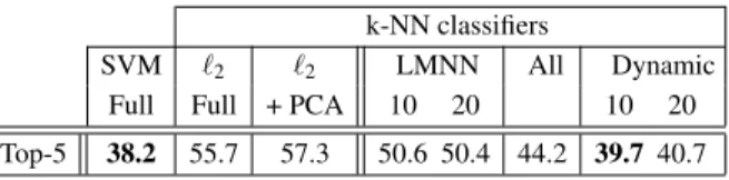
The results in Table2show that all methods lead to metrics that are better than the ℓ2metric in the original space, or after a PCA projection to 128 dimensions.
k-NN classifiers
SVM ℓ2 ℓ2 LMNN All Dynamic
Full Full + PCA 10 20 10 20 Top-5 38.2 55.7 57.3 50.6 50.4 44.2 39.7 40.7
Table 2: Comparison of flat error for different k-NN classification methods using 4K dimensional features. For all methods, except those indicated by ‘Full’, the data is projected to a 128 dimensional space.
Furthermore, we can improve over LMNN by using all within-class images as tar-gets, or even further by using dynamic targets. The success of the dynamic target selection can be explained by the fact that among the three alternatives, the learning objective is the most closely related to the k-NN classification rule. The best perfor-mance on the flat top-5 error of 39.7 using 10 dynamic targets is, however, slightly worse than the 38.2 error rate of the SVM baseline.
5.2.2 Impact of projection dimension on k-NN classification
Next, we evaluate the influence of the projection dimensionalityd on the perfor-mance, by varyingdbetween 32 and 1024. We only show results using 10 dynamic targets, since this performed best among the evaluated k-NN methods. From the re-sults in Table3we see that a projection to 256 dimensions yields the lowest error of 39.0, which still remains somewhat inferior to the SVM baseline.
5.3 Nearest class mean classifier results
We now consider the performance of NCM classifiers and the related methods de-scribed in Section3. In Table3we show the results for various projection dimen-sionalities.
We first consider the results for the 4K dimensional features. As observed for the k-NN classifier, using a learned metric outperforms using theℓ2distance (68.0), which is far worse than using the k-NN classifier (55.7, see Table2). However, un-expectedly, with metric learning we observe that our NCM classifier (37.0) outper-forms the more flexible k-NN classifier (39.0), as well as the SVM baseline (38.2) when projecting to 256 dimensions or more. Our implementation of WSABIE [46] scores slightly worse (38.5) than the baseline and our NCM classifier, and does not generalize to new classes without retraining.
We also compare our NCM classifier to several algorithms which do allow gener-alization to new classes. First, we consider two other supervised metric learning ap-proaches, NCM with FDA (which leads to 50.2) and ridge-regression (which leads to 54.6). We observe that NCMML outperforms both methods significantly.
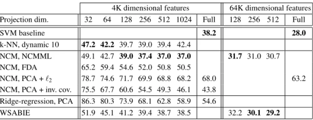
Sec-4K dimensional features 64K dimensional features Projection dim. 32 64 128 256 512 1024 Full 128 256 512 Full
SVM baseline 38.2 28.0
k-NN, dynamic 10 47.2 42.2 39.7 39.0 39.4 42.4
NCM, NCMML 49.1 42.7 39.0 37.4 37.0 37.0 31.7 31.0 30.7 NCM, FDA 65.2 59.4 54.6 52.0 50.8 50.5
NCM, PCA +ℓ2 78.7 74.6 71.7 69.9 68.8 68.2 68.0 63.2
NCM, PCA + inv. cov. 75.5 67.7 60.6 54.5 49.3 46.1 43.8 Ridge-regression, PCA 86.3 80.3 73.9 68.1 62.8 58.9 54.6
WSABIE 51.9 45.1 41.2 39.4 38.7 38.5 32.2 30.1 29.2
Table 3: Flat top-5 error of k-NN and NCM classifiers, as well as baselines, us-ing the 4K and 64K dimensional features, for various projection dimensions, and comparison to related methods, see text for details.
ond, we consider two unsupervised variants of the NCM classifier where we use PCA to reduce the dimensionality. In one case we use theℓ2metric after PCA. In the other, inspired by ridge-regression, we use NCM with the metricWgenerated by the inverse of the regularized covariance matrix, such thatW⊤W = (Σ+λI)−1, see Section3.2. We tuned the regularization parameterλ on the validation set, as was also done for ridge-regression. From these results we can conclude that, just like for k-NN, theℓ2metric with or without PCA leads to poor results (68.0) as compared to a learned metric. Also, the feature whitening implemented by the inverse covariance metric leads to results (43.8) that are better than using theℓ2metric, and also sub-stantially better than ridge-regression (54.6). The results are however significantly worse than using our learned metric, in particular when using low-dimensional pro-jections.
When we use the 64K dimensional features, the results of the NCM classifier (30.8) are somewhat worse than the SVM baseline (28.0); again the learned metric is significantly better than using theℓ2distance (63.2). WSABIE obtains an error of 29.2, in between the SVM and NCM.
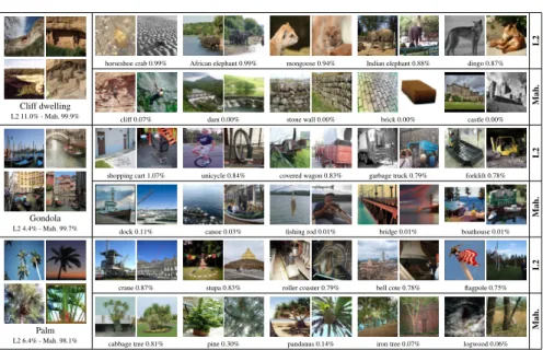
5.3.1 Illustration of metric learned by NCMML.
In Figure7we illustrate the difference between theℓ2and the Mahalanobis metric induced by a learned projection from 64K to 512 dimensions. For three reference classes we show the five nearest classes, based on the distance between class means. We also show the posterior probabilities on the reference class and its five neighbor classes according to Eq. (5). The feature vectorxxxis set as the mean of the reference class,i.e. a simulated perfectly typical image of this class. For theℓ2metric, we used our metric learning algorithm to learn a scaling of theℓ2metric to minimize Eq. (9). This does not change the ordering of classes, but ensures that we can compare prob-abilities computed using both metrics. We find that, as expected, the learned metric
Cliff dwelling L2 11.0% - Mah. 99.9%
horseshoe crab 0.99% African elephant 0.99% mongoose 0.94% Indian elephant 0.88% dingo 0.87%
L2
cliff 0.07% dam 0.00% stone wall 0.00% brick 0.00% castle 0.00%
Mah.
Gondola L2 4.4% - Mah. 99.7%
shopping cart 1.07% unicycle 0.84% covered wagon 0.83% garbage truck 0.79% forklift 0.78%
L2
dock 0.11% canoe 0.03% fishing rod 0.01% bridge 0.01% boathouse 0.01%
Mah.
Palm L2 6.4% - Mah. 98.1%
crane 0.87% stupa 0.83% roller coaster 0.79% bell cote 0.78% flagpole 0.75%
L2
cabbage tree 0.81% pine 0.30% pandanus 0.14% iron tree 0.07% logwood 0.06%
Mah.
Fig. 7: The nearest classes for two reference classes using the theℓ2distance and metric learned by NCMML. Class probabilities are given for a simulated image that equals the mean of the reference class, see text for details.
has more visually and semantically related neighbor classes. Moreover, we see that using the learned metric most of the probability mass is assigned to the reference class, whereas theℓ2metric leads to rather uncertain classifications.
5.3.2 Non-linear classification using multiple class centroids.
In these experiments we use the non-linear NCMC classifier, introduced in Sec-tion 3.3, where each class is represented by a set of kcentroids. We obtain thek centroids per class by using thek-means algorithm in theℓ2space.
Since the cost of training these classifiers is much higher, we run two sets of experiments. In Figure8, we show the performance of using the NCMC classifier only at test time withk= [2, . . . ,30], while using a metric obtained by the NCM objective (k=1). This method is denoted as NCMC-test. In Table4, we show the performance of the NCMC classifier, trained with the NCMC objective, using the 4K features. In the same table we compare the results to the NCM method and the best NCMC-test method.
From the results we observe that a significant performance improvement can be made by using the non-linear NCMC classifier, especially when using a low number of projection dimensionalities. When learning the NCMC classifier we can further improve the performance of the non-linear classification, albeit for a higher training cost. When using as little as 512 projection dimensions, we obtain a performance of
0 5 10 15 20 25 30 36 37 38 39 128d 256d 512d 1024d 0 5 10 15 20 25 30 29 .5 30 30 .5 31 31 .5 32 128d 256d 512d
Fig. 8: The flat top-5 error of the NCMC-test classifier, which at test time uses k>1 on a metric obtained withk=1, for the 4K features (left) and the 64k (right) features. NCM NCMC-test NCMC Proj. Dim. (k) 5 10 15 128 39.0 36.3 (30) 36.2 35.8 36.1 256 37.4 36.1 (20) 35.0 34.8 35.3 512 37.0 36.2 (20) 34.8 34.6 35.1
Table 4: The flat top-5 error of the NCMC classifier using the 4K features, compared to the NCM baseline and the best NCMC-test classifier (withkin brackets).
34.6 on the top-5 error, usingk=10 centroids. That is an improvement of about 2.4 absolute points over the NCM classifier (37.0), and 3.6 absolute points over SVM classification (38.2),c.f. Table3.
For the 64K features learning for the NCMC objective (with,k=10 andd=512) improves the performance to 29.4, about 1.3 points over the NCM classifier.
5.4 Generalizing to new classes with few samples
Given the encouraging classification accuracy of the NCM classifier observed above —and its superior efficiency as compared to the k-NN classifier— we now explore its ability to generalize to novel classes. We also consider its performance as a func-tion of the number of training images available to estimate the mean of novel classes.
Generalization to classes not seen during training.
In this experiment we use approximately 1M images corresponding to 800 random classes to learn metrics, and evaluate the generalization performance on 200
held-4K dimensional features 64K dimensional features
SVM k-NN NCM SVM NCM
Projection dim. Full 128 256 ℓ2 128 256 512 1024 ℓ2 Full 128 256 512 ℓ2
Trained on all 37.6 39.0 38.4 38.6 36.8 36.4 36.5 27.7 31.7 30.8 30.6 Trained on 800 42.2 42.4 54.2 42.5 40.4 39.9 39.6 66.6 39.3 37.8 37.8 61.9
Table 5: Flat top-5 error for 1,000-way classification among test images of 200 classes not used for metric learning, and control setting with metric learning using all classes.
4K dimensional features 64K dimensional features Previous Results
Method NCM SVM NCM SVM [9] [39] [35] [26]
Proj. dim. 128 256 512 1024 Full Full 128 256 512 Full Full 21K 128K 128K Top-1 err. 91.8 90.6 90.5 90.4 95.5 86.0 87.1 86.3 86.1 93.6 78.1 93.6 83.3 80.9 80.8 Top-5 err. 80.7 78.7 78.6 78.6 89.0 72.4 71.7 70.5 70.1 85.4 60.9
Table 6: Flat error rate of the NCM classifier on the ImageNet-10K dataset, us-ing metrics learned on the ILSVRC’10 dataset, with comparison to the baseline SVM, the NCM usingℓ2distance (denoted as full), and previously reported SVM results [9,39,35] and the Deep Learning framework of [26].
out classes. The error is evaluated in a 1,000-way classification task, and computed over the 30K images in the test set of the held-out classes. The early stopping strat-egy uses the validation set of the 200 unseen classes. Performance among test im-ages of the 800 train classes changes only marginally and would obscure the changes among the test images of the 200 held-out classes.
In Table5we show the performance of NCM and k-NN classifiers, and compare it to the control setting where the metric is trained on all 1,000 classes. The results show that both classifiers generalize remarkably well to new classes. For compari-son we also include the results of the SVM baseline, and the k-NN and NCM clas-sifiers using theℓ2distance, evaluated over the 200 held-out classes. In particular for 1024 dimensional projections of the 4K features, the NCM classifier achieves an error of 39.6 over classes not seen during training, as compared to 36.5 when using all classes for training. For the 64K dimensional features the drop in performance is larger, but still surprisingly good considering that training for the novel classes consists only in computing their means.
To further demonstrate the generalization ability of the NCM classifier using learned metrics, we also compare it against the SVM baseline on the ImageNet-10K dataset. We use projections learned and validated on the ILSVRC’10 dataset, and only compute the means of the 10K classes. The results in Table6show that even in this extremely challenging setting the NCM classifier performs remarkably well compared to earlier mentioned SVM-based results of [9,39,35] and our baseline, all of which require training 10K classifiers. We note that, to the best of our knowledge,