A framework to generate synthetic multi-label datasets

Universidade de São Paulo

2014-02-25

A framework to generate synthetic multi-label

datasets

Electronic Notes in Theoretical Computer Science, Amsterdam, v.302, p.155-176, 2014

http://www.producao.usp.br/handle/BDPI/44788

Downloaded from: Biblioteca Digital da Produção Intelectual - BDPI, Universidade de São Paulo

A Framework to Generate

Synthetic Multi-label Datasets

Jimena Torres Tom´as

Newton Spolaˆor

Everton Alvares Cherman

Maria Carolina Monard

a _{Laboratory of Computational Intelligence}

Institute of Mathematics and Computer Science University of S˜ao Paulo

13560-970 S˜ao Carlos, SP, Brazil

Abstract

A controlled environment based on known properties of the dataset used by a learning algorithm is useful to empirically evaluate machine learning algorithms. Synthetic (artificial) datasets are used for this purpose. Although there are publicly available frameworks to generate synthetic single-label datasets, this is not the case for multi-label datasets, in which each instance is associated with a set of labels usually correlated. This work presentsMldatagen, a multi-label dataset generator framework we have implemented, which is publicly available to the community. Currently, two strategies have been implemented inMldatagen: hypersphere and hypercube. For each label in the multi-label dataset, these strategies randomly gener-ate a geometric shape (hypersphere or hypercube), which is populgener-ated with points (instances) randomly generated. Afterwards, each instance is labeled according to the shapes it belongs to, which defines its multi-label. Experiments with a multi-label classification algorithm in six synthetic datasets illustrate the use ofMldatagen.

Keywords: data generator, artificial datasets, multi-label learning, publicly available framework, Java, PHP

1

Introduction

Classical supervised learning algorithms are single-label, in which only one label from a disjoint set of labelsLis associated to each example in the dataset. IfL= 2, the task is called binary classification, and it is called multi-class classification if

1 _{This research was supported by the S˜ao Paulo Research Foundation (FAPESP), grants 2011/02393-4,} 2010/15992-0 and 2011/12597-6. The authors would like to thank Victor Augusto Moraes Carvalho for his help in additional analysis, as well as the anonymous reviewers for their helpful comments.

2 _{Email: jimenat.tomas@gmail.com} 3 _{Email: newtonspolaor@gmail.com} 4 _{Email: echerman@icmc.usp.br} 5 _{Email: mcmonard@icmc.usp.br}

Available online at www.sciencedirect.com

Electronic Notes in Theoretical Computer Science 302 (2014) 155–176

1571-0661/© 2014 Elsevier B.V. All rights reserved.

www.elsevier.com/locate/entcs

L >2. However, an increasing number of applications in which examples are anno-tated using more than one label, such as bioinformatics, emotion analysis, semantic annotation of media and text mining [15], requires different algorithms to extract patterns from data. These applications, in which the examples can be associated to several labels simultaneously, characterize a multi-label learning problem.

In practice, the effectiveness of machine learning algorithms depends on the quality of the generated classifiers. This makes fundamental research in machine learning inherently empirical [6]. To this end, the community carries out exten-sive experimental studies to evaluate the performance of learning algorithms [9]. Synthetic (artificial) datasets are useful in these empirical studies, as they offer a controlled environment based on known properties of the dataset used by the learn-ing algorithm to construct the classifier [2]. A good classifier is generally considered to be one that learns to correctly identify the label(s) of new examples with a high probability. Thus, synthetic datasets can be used instead of real world datasets to derive rigorous results for the average case performance of learning algorithms.

Several frameworks to generate synthetic single-label datasets are publicly avail-able to the community6 7 8. However, despite some proposals of strategies to generate synthetic multi-label datasets [17,18,3,11], to the best of our knowl-edge, there is a lack of publicly available frameworks to generate data for multi-label learning. Thus, this work contributes to bridging this gap by proposing

the Mldatagen framework, which we have implemented and it is hosted at http:

//sites.labic.icmc.usp.br/mldatagen.

The remainder of this work is organized as follows: Section 2 briefly de-scribes multi-label learning concepts and strategies to generate synthetic multi-label datasets. The proposed framework is presented in Section3and illustrated in Sec-tion 4. Section5presents the conclusions and future work.

2

Background

This section presents basic concepts and terminologies related to multi-label learn-ing, including the evaluation measures used in this work, as well as some strategies proposed in the literature to generate synthetic multi-label datasets.

2.1 Basic concepts of multi-label learning

LetD be a dataset composed ofN examplesE_i= (xi, Yi),i= 1..N. Each example

(instance) E_i is associated with a feature vector xi = (xi1, xi2, . . . , xiM) described

by M features (attributes) X_j, j = 1..M, and a subset of labels Y_i ⊆ L, where

L = {y₁, y₂, . . . y_q} is the set of q labels. Table 1 shows this representation. In this scenario, the multi-label classification task consists in generating a classifierH

which, given an unseen instance E = (x,?), is capable of accurately predicting its subset of labels (multi-label)Y, i.e.,H(E)→Y.

6 _{http://archive.ics.uci.edu/ml/machine-learning-databases/dgp-2} 7 _{http://www.datasetgenerator.com}

Table 1 Multi-label data. X₁ X₂ . . . X_M Y E₁ x₁₁ x₁₂ . . . x_1M Y₁ E₂ x₂₁ x₂₂ . . . x_2M Y₂ .. . ... ... . .. ... ... E_N x_N1 x_N2 . . . x_{N M} Y_N

Multi-label learning methods can be organized into two main categories: algo-rithm adaptation and problem transformation [15]. The first one consists of methods which extend specific learning algorithms to handle multi-label data directly, such as the Multi-label Naive Bayes (MLNB) algorithm [18]. The second category is algorithm independent, allowing one to use any state of the art single-label learn-ing method. Methods which transform the multi-label classification problem into several single-label classification problems, such as the Binary Relevance (BR) ap-proach, fall within this category. Specifically,BR transforms a multi-label dataset intoq single-label datasets, classifies each single-label problem separately and then combines the outputs.

2.1.1 Evaluation measures

The evaluation of single-label classifiers has only two possible outcomes, correct or incorrect. However, evaluating multi-label classification should also take into account partially correct classification. To this end, several multi-label evaluation measures have been proposed, as described in [15]. In what follows, we briefly describe the example-based and label-based evaluation measures used in this work. All these performance measures range in [0..1].

Example-based evaluation measures Let Δ be the symmetric difference between two sets; Yi andZi be, respectively, the set of true and predicted labels;

I(true) = 1 and I(false) = 0. The Hamming-Loss, Subset-Accuracy, Precision,

Hamming Loss(H, D) = 1 N N i=1 |YiΔZi| |L| . (1) Subset Accuracy(H, D) = 1 N N i=1 I(Zi=Yi). (2) P recision(H, D) = 1 N N i=1 |Yi∩Zi| |Z_i| . (3) Recall(H, D) = 1 N N i=1 |Yi∩Zi| |Y_i| . (4) Accuracy(H, D) = 1 N N i=1 |Y_i∩Z_i| |Y_i∪Z_i|. (5)

Unlike all other evaluation measures described in this section, for

Hamming-Loss, the smaller the value, the better the multi-label classifier

perfor-mance is. Moreover, it is worth observing that Subset-Accuracy is a very strict evaluation measure as it requires an exact match of the predicted and the true set of labels.

Label-based evaluation measures In this case, for each single-label y_i ∈L, theqbinary classifiers are initially evaluated using any one of the binary evaluation measures proposed in the literature, such as Accuracy, F-Measure, ROC and others, which are afterwards averaged over all labels. Two averaging operations, macro-averaging and micro-macro-averaging, can be used to average over all labels.

Let B(TP_yi, FP_yi, TN_yi, FN_yi) be a binary evaluation measure calculated for a

label yi based on the number of true positive (TP), false positive (FP), true

nega-tive (TN) and false negative (FN). The macro-average version of B is defined by

Equation 6and the micro-average by Equation7.

Bmacro= 1 q q i=1 B TP_yi, FP_yi, TN_yi, FN_yi . (6) Bmicro=B _q i=1 TP_yi, q i=1 FP_yi, q i=1 TN_yi, q i=1 FN_yi . (7)

Thus, the binary evaluation measure used is computed on individual labels first and then averaged for all labels by the macro-averaging operation, while it is com-puted globally for all instances and all labels by the micro-averaging operation. This means that macro-averaging would be more affected by labels that partici-pate in fewer multi-labels, i.e., fewer examples, which is appropriate in the study of unbalanced datasets [5].

In this work, we use Precision (PC), Recall (RL) and F-Measure (FM), defined by Equations8to 10respectively, as binary evaluation measures.

P C(H, D) = TP

TP+FP

. (8) RL(H, D) = TP

TP +FN

F M(H, D) = 2TP

2T_P +F_P +F_N. (10)

2.2 Strategies to generate synthetic multi-label datasets

As already mentioned, few strategies to generate synthetic multi-label datasets have been proposed in the literature. In what follows, some of these strategies are briefly described.

In [3] it is proposed to build a synthetic multi-label dataset based on specific functions to label instances which extends an earlier proposal for single-label learn-ing [1]. Many of theM = 9 features of the dataset are defined according to uniform distribution.

Synthetic datasets with different properties are generated in [11] to study multi-label decision trees. In this study, the power to identify good features, related to the feature selection task [10], was also verified. The strategy used to generate the datasets considers several functions to define feature values related to the labels.

To illustrate a new multi-label learning algorithm, a synthetic dataset is specified in [17]. Given three labels and a covariance matrix, instances are labeled according to seven Gaussian distributions, such that each distribution is related to one multi-label. The number of instances per multi-label is arbitrarily defined.

Hyperspheres are used to generate twelve synthetic datasets in [18]. First, a hypersphere HS with radius r is generated in RM2 . For each label in a dataset, a smaller hypersphere hsi, i = 1..q, is also randomly generated. Then, the small

hyperspheres are populated with points (instances) randomly generated. The di-mension of these points increases by adding M₄ irrelevant features, with random values, and M₄ redundant ones, which copy the original features. Finally, each in-stanceEi is labeled according to the small hyperspheres it belongs to, which define

the multi-labelYi.

3

Synthetic multi-label dataset generator proposed

Mldatagen, implemented in Java9 and PHP10.

The framework outputs a compressed file which contains a noiseless synthetic dataset with the characteristics specified by the user, as well as similar datasets in which noise has been inserted. Mldatagen will generate as many datasets with noise as the number of different noise levels requested by the user. Each dataset is in the Mulan format11, which consists of two files: an ARFF file and a XML file. These

9 _{http://www.oracle.com/technetwork/java/index.html} 10_{http://php.net}

files can be directly submitted to the multi-label learning algorithms available in the Mulan library [16].

3.1 The HyperSpheres strategy

This strategy has 9 input parameters to generate datasets withM =M_rel+M_irr+

M_red features.

• M_rel - Number of relevant features.

• M_irr - Number of irrelevant features.

• M_red - Number of redundant features.

• q - Number of labels in the dataset.

• N - Number of instances in the dataset.

• maxR- Maximum radius of the small hyperspheres.

• minR- Minimum radius of the small hyperspheres.

• μ- Noise level(s).

• name - Name of the relation in the header of the ARFF file.

As mentioned, a dataset with noise is generated by Mldatagen for each noise level. Moreover, the optional parameters maxR, minR, μandname have default values inMldatagen, as described in Section3.3.

To prevent the user setting invalid values, the following constraints are assigned to the parameters.

Mrel >0 q >0 minR >0 minR < maxR≤0.8

M_irr≥0 N >0 μ≥0 0< minR≤

q

10+ 1

q

Mred≥0 maxR >0 Mred≤Mrel

It should be emphasized that Mldatagen extends the strategy proposed in [18] by enabling the user to choose the number of different kinds of features, i.e., rel-evant, irrelevant and redundant, the maximum and minimum radius of the small hyperspheres, as well as the noise level of the datasets generated.

The main steps to generate the synthetic datasets are: (i) Generating the hypersphereHS inRMrel_.

(ii) Generating theq small hyperspheres hsi,i= 1..q insideHS.

(iii) Generating theN points (instances) inRM.

(iv) Generating the multi-labels based on the q small hyperspheres and inserting the noise level(s)μ.

3.1.1 Generating the hypersphereHS

A hypersphere HS in RMrel_{, centered on the origin of the Cartesian coordinate}

system and with radiusr_HS = 1, is created.

3.1.2 Generating theq small hyperspheres

All the small hyperspheres are generated in such a way that they are inside the hypersphereHSinRMrel_{. In addition, each hyperspherehsi= (ri, Ci) is defined by}

a specific radiusri and centerCi= (ci1, ci2, ci3, . . . , ciM_rel). This radius is randomly

generated and ranges fromminRtomaxR. On the other hand, theCi coordinates

must fulfill the initial requirement defined by Equation 11 to generate hsi inside

HS.

∀i∈[1..q] cij ≤(1−ri), j= 1..Mrel. (11)

Nevertheless, this requirement is insufficient to ensure thaths_iis insideHS. For example, if a valuec_i1 = (1−r_i) were generated, the otherc_ij values forj= 1 would be zero,i.e., the remainingM_rel−1 features have to be zero. Thus, all coordinates of eachC_i,i= 1..q, must range in the restricted domain defined by Equation12.

M_rel j=1

cij2≤(1−ri)2. (12)

The filled area in Figure 1 shows the domain of the Ci coordinates of a

hyper-spherehsi forMrel= 2, such that hsi is insideHS.

Fig. 1. Domain to defineCi, givenri, inR2

As specified in Equation 12, setting the coordinates of Ci, i = 1..q, must take

into account its radius ri, as well as the already set coordinate values of the hsi

hypersphere center. This requirement is defined by Equation13for each randomly generated coordinate cij, j= 1..Mrel, in which only coordinates cis, s=j, already

set are considered.

− (1−ri)2− Mrel s=1,s=j (cis)2 ≤cij ≤ (1−ri)2− Mrel s=1,s=j (cis)2. (13)

As the possible range to define each coordinate of Ci reduces whenever a new

coordinate is set, it is necessary to avoid determinism during the generation of the

Ci coordinates of the hypersphere hsi, i.e., to avoid always generating ci1 as the

first coordinate andciM_rel as the last one. To this end, the index of the coordinates

j to be set,j= 1..M_rel, is randomly defined.

Algorithm 1 summarizes the generation of the hypersphereshs_i = (r_i, C_i), i = 1..q. In this algorithm, the function random(x, y) outputs a value ranging from

x to y according to the uniform distribution. The functions updateminC(x) and

updatemaxC(x) respectively refresh the lower and upper bounds of the next C_i

coordinate to be defined using Equation 13. These procedures are useful to avoid generating instances with empty multi-labels.

Algorithm 1 Generation of the small hyperspheres

1: for i= 1→q do 2: C_i ← ∅

3: r_i ←random(minR, maxR) 4: maxC←(1−ri)

5: minC ← −(1−ri)

6: for j= 1→M_rel (j randomly def ined)do 7: cij ←random(minC, maxC)

8: Ci ←Ci∪ {cij}

9: minC ←updateminC(minC)

10: maxC←updatemaxC(maxC)

11: end for 12: hsi←(ri, Ci)

13: end for

14: return {hs1, hs2, . . . , hsq}

3.1.3 Generating the points

After defining the q small hyperspheres, the main hypersphere HS is populated with N points (instances). Recall that in each instance Ei = (xi, Yi), i = 1..N,

xi denotes the vector of feature values and Yi ⊆L the multi-label of the instance.

Thus, to populateHSinRM, it is required to generate the values (xi1, xi2, . . . , xiM)

and the multi-label Yi for each instanceEi.

To ensure that the multi-labels contain at least one of theq possible labels, the generation of theN instances is oriented, such that, for each instanceE_i, the point with coordinates (x_i1, x_i2, . . . , x_iMrel) is at least inside one small hypersphere. By using this procedure, none of the instances will have an empty multi-label. All small hypersphereshs_i, i= 1..q, are populated using this criterion.

Moreover, as the radiuses of the small hyperspheres are different, the distribution (balance) of instances in each hypersphere should be kept, i.e., an hypersphere with greater radius should be proportionally more crowded than an hypersphere with smaller radius. To this end, the framework uses the balance factor defined by Equation 14. Therefore, Ni = round(f ×ri) points are generated inside each

hyperspherehsi, i= 1..q.

f = _qN

i=1ri

. (14)

As the procedure to generate the small hypersphere centers does, a random point x_k = (x_k1, x_k2, . . . , x_kMrel) inside hsi = (ri, Ci) must be generated obeying

the restrictions given by Equation15.

Mrel

j=1

(x_kj−c_ij)2≤r2_i. (15) However, the domain to generate the x_k coordinates is different, and is reduced to the region inside hs_i. As the hs_i center is not on the origin, it is required to take into account the coordinates of this center. Figure2exemplifies, forM_rel= 2, that a random pointx_k must be inside the filled area to belong to the hypersphere

hs_i = (r_i, C_i).

Fig. 2. Domain to definexk, givenriandCi, inR2

Therefore, to randomly generate each coordinate x_kj, j = 1..M_rel, of point x_k, it is required to assure that |x_kj−c_ij| ≤ r_i. However, in an extreme case, if the first coordinate were x_k1 = c_i1+r_i, then the remaining x_kj values, j = 1, would be mandatorily equal to c_ij to ensure that point x_k is inside hs_i. Thus, the x_kj

coordinate, ∀j ∈[1..M_rel], should be randomly generated taking into account the already set coordinates. To this end, the range should be constrained as defined by Equation16for each randomly generated coordinatex_kj, j = 1..M_rel, in which only coordinatesx_ks, s=j, already set are considered.

cij− r_i2− Mrel s=1,s=j (xks−cis)2 ≤xkj≤cij+ r2_i − Mrel s=1,s=j (xks−cis)2, ∀i∈[1..q]e∀k∈[1..N]. (16) As the procedure to generate the Ci coordinates does, it is required to avoid

determinism during the specification of the coordinates of point xk, i.e., to avoid

always generatingxk1 as the first coordinate andxkMrel as the last one. Thus, the

Algorithm 2 summarizes the generation of the instances x_k, k = 1..N, in-side the small hyperspheres hsi = (ri, Ci), i = 1..q. Similar to Algorithm 1, the

updateminX(x) andupdatemaxX(x) functions refresh respectively the lower and upper bounds of the nextx_k coordinate to be defined inside the corresponding hy-perspherehsi. The already set coordinates are also taken into account to randomly

generate the remaining coordinates.

Algorithm 2 Generation of the points inside the hyperspheres

1: for k= 1→N do 2: xk ← ∅

3: maxX←cij −ri

4: minX ←cij+ri

5: for j= 1→Mrel (j randomly def ined)do

6: xkj ←random(minX, maxX)

7: xk←xk∪ {xkj}

8: minX ←updateminX(minX)

9: maxX←updatemaxX(maxX)

10: end for 11: end for

12: return {x1,x2, . . . ,xN}

After generating theN points related toM_rel,M_irrandM_redfeatures are set by addingM_irr irrelevant features, with random values, and M_red redundant features. The features to be replicated as redundant are chosen randomly. In the end, theN

points are inRM_{, M =M}

rel+Mirr+Mred.

3.1.4 Generating the multi-labels

Any instancex_k ∀k ∈[1..N] has the labely_i, i= 1..q, in its multi-labelY_k, if x_k is inside the hypersphere hs_i. The final multi-label Y_k consists of all labels fulfilling this condition, which can be easily verified according to the distance between x_k

and each center C_i, i= 1..q. If this distance is smaller than the radiusr_i, then x_k

is inside hs_i and y_i ∈Y_k; otherwise, y_i ∈/ Y_k. The procedure to assign the labely_i

to the multi-label Y_k of x_k ∀k ∈[1..N] is implemented as defined by Equation 17. Note that only theM_rel features have to be considered.

(x_kj−c_ij)2_≤r

i, (17)

∀i∈[1..q], ∀j∈[1..M_rel],∀k∈[1..N].

After constructing this dataset, if requested by the user, the noisy dataset(s) are generated. To this end, for each instance E_i, the procedure to insert noise in the constructed dataset flips the label y_j ∈ Y_i, j = 1..q, with probability μ. In other words, if the label y_j is in the multi-label Y_i, the flip will remove y_j from the multi-label Y_i with probabilityμ. Otherwise, the labely_j will be inserted with probabilityμ.

Based on theHyperSpheres strategy, we propose a similar strategy named

3.2 The HyperCubes strategy

The main motivation behind this strategy is that hypercubes could be appropriate to evaluate multi-label learning algorithms, such as decision trees [4], which classify instances by dividing the space using hyperplanes.

The HyperCubes strategy also has 9 parameters and the corresponding

con-straints to generate synthetic datasets without and with noise. However, different from the HyperSpheres strategy, maxR and minR denote, respectively, the maxi-mum and minimaxi-mum half-edges (edge₂ ) of the small hypercubes.

The main steps considered to generate synthetic datasets according to the

Hy-perCubes strategy are similar to the ones required byHyperSpheres.

(i) Generating the hypercube HC in RMrel_.

(ii) Generating the q small hypercubeshc_i, i= 1..q insideHC. (iii) Generating theN points (instances) inRM_.

(iv) Generating the multi-labels based on theq small hypercubes and inserting the noise level(s) μ.

3.2.1 Generating the hypercube HC

A hypercubeHCinRMrel_{, centered on the origin of the Cartesian coordinate system}

with half-edgeeHC = 1, is created.

3.2.2 Generating theq small hypercubes

As HyperSpheres does, HyperCubes generates q small hypercubes hci = (ei, Ci),

i = 1..q, such that they are inside HC in RMrel_{. Each small hypercube is defined}

by a specific half-edge ei and center Ci = (ci1, ci2, ci3, . . . , ciMrel). This half-edge is

randomly generated and ranges fromminR to maxR. On the other hand, the Ci

coordinates must fulfill the initial requirement defined by Equation 18to generate

hci insideHC.

∀i∈[1..q] cij ≤(1−ei), j= 1..Mrel. (18)

Different from HyperSpheres, this requirement is enough to ensure that hc_i is inside HC. Therefore, the domain in which the C_i coordinates range is given by Equation18. The filled area in Figure3shows the domain of theC_i coordinates of a hypercubehc_i forM_rel= 2, such that hc_i is insideHC.

Different from HyperSpheres, the possible ranges to define each coordinate cij

are the same for all coordinates. Thus, Algorithm3is simpler than Algorithm1, as the functionsupdateminC(x) andupdatemaxC(x) are not needed to generate the hypercubeshci= (ei, Ci),i= 1..q.

3.2.3 Generating the points

As HyperSpheres does, after defining theq small hypercubes, the main hypercube

HC is populated withN points (instances). To populateHC inRM, it is required to generate the values (xi1, xi2, . . . , xiM) and the multi-label Yi for each instance

Fig. 3. Domain to defineCi, givenei, inR2

Algorithm 3 Generation of the small hypercubes

1: for i= 1→q do 2: C_i ← ∅

3: e_i ←random(minR, maxR) 4: maxC←(1−e_i)

5: minC ← −(1−e_i) 6: for j= 1→M_rel do

7: c_ij ←random(minC, maxC) 8: C_i ←C_i∪ {c_ij} 9: end for 10: hc_i←(e_i, C_i) 11: end for 12: return {hc₁, hc₂, . . . , hc_q} Ei.

In addition, HyperCubes also oriented the generation of points, such that each point is at least inside one small hypercube. By using this procedure, no instances have empty multi-labels and all small hypercubes hc_i,i= 1..q, are populated.

To ensure that the distribution of instances inside each small hypercube is pro-portional to the corresponding half-edge, the framework uses a balance factor similar to the one in Equation 14. However, instead of summing radiuses, half-edges are summed. Thus,Ni=round(f×ei) points are generated inside each hypercubehci,

i= 1..q.

As the procedure to generate the small hypercube centers does, a random point

x_k = (x_k1, x_k2, . . . , x_kMrel) inside hc_i = (e_i, C_i) must be generated as defined by Equation 19.

|(xkj−cij)| ≤ei,∀i∈[1..q]e∀j∈[1..Mrel]. (19)

Similar to Section 3.1.3, the domain to generate thexk coordinates is different,

being reduced to the region inside hci. As the hci center is not on the origin, it is

required to take into account the coordinates of this center. Figure 4 exemplifies, forMrel = 2, that a random pointxk must be inside the filled area to belong to the

Fig. 4. Domain to definexk, givenei, inR2

Algorithm 4 summarizes the generation of the instances xk, k = 1..N, inside

a small hypercube hci = (ei, Ci), i = 1..q. This algorithm is simpler than

Algo-rithm 2 by discarding the functions updateminX(x) and updatemaxX(x), as the coordinates range in the same domain.

Algorithm 4Generation of the points inside the hypercubes

1: fork= 1→N do 2: x_k ← ∅

3: maxX←c_ij−e_i 4: minX←c_ij+e_i 5: forj= 1→M_rel do

6: x_kj←random(minX, maxX) 7: x_k ←x_k∪ {x_kj}

8: end for 9: end for

10: return {x₁,x₂, . . . ,x_N}

As HyperSpheres does, after generating the N points related toM_rel, the M_irr

andM_red features are set by adding M_irr irrelevant features, with random values, andM_redredundant features. The features to be replicated as redundant are chosen randomly. In the end, theN points are inRM_{,M =M}

rel+Mirr+Mred.

3.2.4 Generating the multi-labels

Similar to HyperSpheres, any instance x_k ∀k ∈ [1..N] has the label yi, i = 1..q,

in its multi-label Y_k, if x_k is inside the hypercube hci. The final multi-label Yk

is thus composed of all labels fulfilling this condition, which can be easily verified according to the distance betweenx_k and each centerCi,i= 1..q. If this distance is

smaller than the half-edgeei, thenxk is insidehci and yi ∈Yk; otherwise,yi∈/Yk.

The procedure to assign the label yi to the multi-label Yk of xk ∀k ∈ [1..N] is

implemented as defined by Equation 20. Note that only the M_rel features have to be considered.

After constructing this dataset, if requested by the user the noisy dataset(s) are generated in the same way as theHyperSpheres strategy does.

3.3 The Mldatagen framework

Currently, both strategies HyperSpheres and HyperCubes (Sections 3.1 and 3.2) are implemented in theMldatagen framework, which is publicly available athttp: //sites.labic.icmc.usp.br/mldatagen. In this web site, the user finds a short introduction to Mldatagen, as well as the interface to configure the framework pa-rameters and download the output.

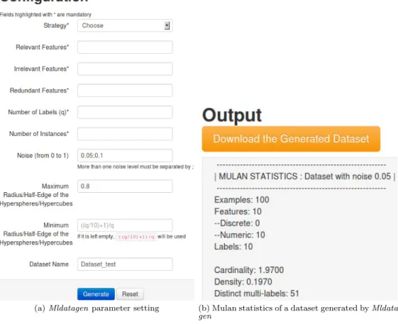
Figure 5a shows the parameter setting interface, which considers mandatory and optional parameters. The user can set one or more noise levels in parameterμ

by separating them with the “;” character. Furthermore, the optional parameters

maxR, minR, μandname have default values: 0.8, (₁₀q + 1)/q, {0.05; 0.1}and “Dataset test”, respectively. After filling in the fields, the user should click on the “Generate” button.

(a)Mldatagenparameter setting (b) Mulan statistics of a dataset generated by

Mldata-gen

Fig. 5. Framework screenshots

To avoid setting invalid values, the constraints described in Section3.1 are ver-ified. If any constraint is not fulfilled, Mldatagen will display an error message indicating the parameter that should be reviewed.

After execution, Mldatagen displays information about the generated dataset, such as the distribution of instances inside the geometrical shape used and multi-label statistics, which are calculated by Mulan, as shown in Figure5b.

To download the Mldatagen output, the user should click on the “Download the generated dataset” button. The output consists of a compressed file named according to the pattern

<x>_<y>_<w>_<z>.tar.gz

in which<x> is the strategy (HyperSpheres or HyperCubes),<y>, <w>and<z> are numbers denoting, respectively, the number of relevant, irrelevant and redundant features. As already mentioned, this compressed file contains the user specified synthetic dataset without noise, as well as one synthetic dataset per noise level set in theμparameter. Each dataset can be directly submitted to Mulan for learning purposes.

4

Illustrative example

Mldatagenwas used to generate 6 synthetic multi-label datasets, 3 using the

Hyper-Spheresstrategy and the other 3 theHyperCubesstrategy. To generate the datasets,

different values of theMrel,MirrandMredparameters were used. These values were

chosen to analyze how the number of features (M = Mrel+Mirr+Mred) and the

number of unimportant features (Mirr andMred) influence the performance of the

multi-labelBRkNN-b learning algorithm [13], available in Mulan. In what follows, information about the synthetic datasets generated,BRkNN-band the classification results are presented.

4.1 Dataset description

The parametersMrel, Mirr andMred were set with different values. Table 2shows

these values and the generation strategy used for each dataset.

Table 2

Number of relevant, irrelevant and redundant features in the six synthetic datasets

Dataset Strategy M_rel M_irr M_red M

A HyperSpheres 20 0 0 20 B HyperCubes 20 0 0 20 C HyperSpheres 10 5 5 20 D HyperCubes 10 5 5 20 E HyperSpheres 5 0 0 5 F HyperCubes 5 0 0 5

Aside the features, Mldatagen was executed with default value parameters, ex-cept for the noise levelμ, the number of instances N and the number of labels q,

which were set as shown in Table3.

Table 3

Setting of otherMldatagen parameters

q N maxR minR μ

10 1000 0.8 (₁₀q + 1)/q 0

Table 4 shows, for each dataset, the single-label frequencies; the lowest and the highest single-label frequencies, as well as the first, second (median) and third quartiles, as suggested by [14]; the Label Cardinality (LC), which is the average number of single-labels associated with each example defined by Equation 21; and the Label Density (LD), which is the normalized cardinality (LD(D) =LC(D)/|L|) defined by Equation 22. LC(D) = 1 |D| |D| i=1 |Yi|. (21) LD(D) = 1 |D| |D| i=1 |Y_i| |L|. (22)

Figure 6 depicts dispersion of the single-label frequencies by boxplots, with a dashed line at frequency = 500 (50%). As can be observed, all single-label frequen-cies are not higher than 50% for datasets A and B. Furthermore, the datasets with less features (E and F) have higher single-label frequencies, with the 3rd quartiles above the dashed line.

A B C D E F

200

400

600

800

Fig. 6. Boxplots of the single-label frequencies

Table 5shows, for each synthetic dataset, the percentage of multi-labels in the dataset with number of labels ranging from 1 to 10. For example, in dataset A, 45.90% of the multi-labels have only one single label, 30.90% have two single-labels and this percentage reduces to 0.50% for 6 single-labels. Moreover, there is no multi-label with more than 6 single-labels.

As can be observed, in the four datasets with M = 20 features, the higher the number of single-labels, the lower the percentage in the multi-label is. On the other hand, the datasetsEandF withM = 5 features show a better frequency distribu-tion. These different behaviors could be explained by the curse of dimensionality [8], which can harm analyses of high-dimensional data.

Table 4

Single-label frequencies and multi-label statistics of the synthetic datasets

Datasets A B C D E F y₁ 65 382 553 109 284 40 y₂ 476 130 63 97 274 633 y₃ 249 94 88 225 729 361 y₄ 69 97 588 67 726 648 y₅ 500 155 78 553 446 810 y₆ 57 209 171 53 210 187 y₇ 151 342 177 75 294 461 y₈ 48 77 468 504 258 55 y₉ 221 66 116 236 577 76 y₁₀ 49 97 69 319 197 326 lowest 48 66 63 53 197 40 1st quartile 59 94.8 80.5 80.5 262 103.8 2nd quartile 110 113.5 143.5 167 289 343.5 3rd quartile 242 195.5 395.3 298.3 544.3 590 highest 500 382 588 553 729 810 LC 1.89 1.65 2.37 2.24 4.00 3.60 LD 0.19 0.17 0.24 0.22 0.40 0.36

4.2 The multi-label BRkNN-b learning algorithm

Lazy algorithms are useful in the evaluation of datasets with irrelevant features, as the classifiers built by these algorithms are usually susceptible to irrelevant features. The multi-label learning algorithmBRkNN is an adaptation of the single-label lazyk

Nearest Neighbor (kNN) algorithm to classify multi-label examples proposed in [13]. It is based on the well-knownBinary Relevanceapproach, which transforms a multi-label dataset intoqsingle-label datasets, one per label. After transforming the data,

kNN classifies each single-label problem separately and thenBRkNN aggregates the prediction of each one of the q single-label classifiers in the corresponding multi-label, which is the one predicted. Despite the similarities between the algorithms,

BRkNN is much faster thankNN applied according to theBRapproach, asBRkNN

Table 5

Percentage of multi-labels with different number of labels

Datasets |Y| A B C D E F 1 45.90 58.60 33.70 37.90 16.20 14.50 2 30.90 25.80 25.70 29.00 16.60 16.70 3 14.40 9.80 20.00 15.20 12.50 20.30 4 6.90 3.90 13.30 10.40 16.40 16.90 5 1.40 1.70 5.20 4.70 11.10 14.20 6 0.50 0.20 1.90 2.40 10.80 10.40 7 0.00 0.00 0.20 0.70 8.20 6.10 8 0.00 0.00 0.00 0.00 5.10 0.90 9 0.00 0.00 0.00 0.00 2.50 0.00 10 0.00 0.00 0.00 0.00 0.60 0.00

To improve the predictive performance and to tackle directly the multi-label problem, the extensions BRkNN-a andBRkNN-b were also proposed in [13]. Both extensions are based on a label confidence score, which is estimated for each label from the percentage of thek nearest neighbors having this label. BRkNN-aclassifies an unseen exampleE using the labels with a confidence score greater than 0.5, i.e., labels included in at least half of thek nearest neighbors ofE. If no label satisfies this condition, it outputs the label with the greatest confidence score. On the other hand, BRkNN-b classifies E with the [s] (nearest integer of s) labels which have the greatest confidence score, where s is the average size of the label sets of the k

nearest neighbors of E.

In this work, we use theBRkNN-bextension proposed in [7] and implemented in Mulan, which was executed withk= 11 and the remaining parameters with default values.

4.3 Results and discussion

All the reported results were obtained by Mulan using 5x2-fold cross-validation, which randomly repeats 2-fold cross-validation five times.

The evaluation measures described in Section 2.1.1 were used to evaluate the classifiers constructed by BRkNN-b. Table 6 shows the average and the standard deviation (in brackets) of the evaluation measure values. The example-based eval-uation measures are denoted in Table6 as: Hamming-Loss (HL); Subset-Accuracy (SAcc); Precision (Pr); Recall (Re); Accuracy (Acc). The label-based evaluation measures are denoted as: Micro-averaged Precision (Pμ); Micro-averaged Recall

(Rμ); Micro-averaged F-Measure (F1μ) and Macro-averaged Recall (RM). Best re-sults among the datasets with M = 20, as well as between the two datasets with

M = 5 are highlighted in gray.

Table 6 Classification performance Example-based measures HL SAcc Pr Re Acc A 0.20 (0.00) 0.06 (0.01) 0.48 (0.01) 0.54 (0.01) 0.37 (0.00) B 0.16 (0.01) 0.12 (0.01) 0.53 (0.01) 0.75 (0.02) 0.47 (0.01) C 0.20 (0.01) 0.08 (0.01) 0.55 (0.02) 0.66 (0.01) 0.45 (0.01) D 0.17 (0.00) 0.10 (0.01) 0.60 (0.01) 0.81 (0.02) 0.52 (0.00) E 0.19 (0.01) 0.12 (0.01) 0.68 (0.01) 0.80 (0.02) 0.61 (0.01) F 0.12 (0.01) 0.23 (0.02) 0.76 (0.01) 0.93 (0.01) 0.71 (0.01) Label-based measures Pμ Rμ F1μ RM A 0.49 (0.01) 0.57 (0.01) 0.52 (0.00) 0.29 (0.01) B 0.52 (0.02) 0.71 (0.02) 0.60 (0.01) 0.73 (0.02) C 0.57 (0.02) 0.69 (0.01) 0.62 (0.01) 0.36 (0.01) D 0.60 (0.01) 0.76 (0.02) 0.67 (0.01) 0.75 (0.02) E 0.73 (0.02) 0.85 (0.01) 0.78 (0.01) 0.78 (0.01) F 0.79 (0.01) 0.91 (0.01) 0.85 (0.01) 0.89 (0.01)

It can be observed that between the two datasets with M = 5 features, dataset

F, which was created using theHyperCubesstrategy, shows the best results. Among the four datasets withM = 20, dataset B obtained the best example-based mea-sure values for Hamming-Loss (HL) and Subset-Accuracy (SAcc), while dataset D

obtained the best results for the remainder of the example-based measures and for all the label-based measures considered. Both datasets were also created using the

HyperCubes strategy.

In what follows, spider graphs summarizing the results of the performance mea-sures in Table 6 (except Hamming-loss) are shown. Thus, greater values indicate better performance. These graphs were generated using the R framework12_.

Fig-ure 7 shows the graphs for datasets A, B, C and D (M = 20), while Figure 8 shows the graphs for datasets E andF (M = 5). Each colored line plots the per-formance of the classifier built with an specific dataset, while each axis represents an evaluation measure.

As stated before, for M = 20 the classifiers build with datasetsB andD show better performance than the ones build with datasets A and C. Moreover, for

M = 5 the classifier build with dataset F shows better results than the one build with dataset E. Observe that these datasets (B, D and F) were generated using

theHyperCubes strategy.

One possible cause of this behavior is that in the HyperSpheres strategy the volume of the main hypersphereHS increases with the dimensionality up to a max-imum value, which depends on the initial volume of the hypersphere. Afterwards, the volume decreases with the dimensionality, tending to zero. As the main hyper-sphereHSused by theHyperSpheres strategy has radius one, its maximum volume

Subset.Accuracy Precision Recall Accuracy 0.2 0.4 0.6 0.8 1 A B C D

(a) Example-based measures

Micro.Precision Micro.Recall Micro.F.Measure Macro.Recall 0.3 0.4 0.5 0.6 0.7 0.8 A B C D (b) Label-based measures Fig. 7. Spider graphs for theA,B,CandDdatasets

Subset.Accuracy Precision Recall Accuracy 0.2 0.4 0.6 0.8 1 E F

(a) Example-based measures

Micro.Precision Micro.Recall Micro.F.Measure Macro.Recall 0.75 0.8 0.85 0.9 0.95 E F (b) Label-based measures Fig. 8. Spider graphs for theEandF datasets

is reached forM = 5, decreasing afterwards. This problem is well described in [12]. On the other hand, in theHyperCubes strategy the volume of the main hypercube

HC always increases with the dimensionality. Both cases are related to the curse of dimensionality.

5

Conclusion

This work proposes two strategies to generate synthetic multi-label datasets. Both strategies were implemented in the framework Mldatagen, which is publicly avail-able, improving the lack of publicly available multi-label generators. Although these

strategies are based on one initial proposal described in [18] for a specific problem, we have extended the initial proposal by offering the user ofMldatagenthe flexibility to choose the number of unimportant features and the noise level for the datasets to be generated, as well as avoiding the occurrence of empty multi-labels. Further-more,Mldatagenoutputs the generated datasets in the Mulan format, a well-known framework for multi-label learning, which is frequently used by the community.

To illustrate Mldatagen, multi-label classifiers were built from six synthetic datasets. The results suggest that the datasets generated by theHyperCubes strat-egy provide better classification results than the ones based on HyperSpheres. In fact, despite both strategies being sensitive to the curse of dimensionality, the vol-ume of a hypercube always increases with the dimensionality, showing better behav-ior than a hypersphere, whose volume decreases from one dimension upwards. As future work, we plan to implement more strategies into the Mldatagen framework and make them available to the community.

References

[1] Agrawal, R., S. Ghosh, T. Imielinski, B. Iyer and A. Swami,An interval classifier for database mining applications, in:International Conference on Very Large Databases, 1992, pp. 560–573.

[2] Bol´on-Canedo, V., N. S´anchez-Maro˜no and A. Alonso-Betanzos,A review of feature selection methods on synthetic data, Knowledge and Information Systems34(2013), pp. 483–519.

[3] Chou, S. and C.-L. Hsu, MMDT: a multi-valued and multi-labeled decision tree classifier for data mining, Expert Systems with Applications28(2005), pp. 799–812.

[4] Clare, A. and R. D. King,Knowledge discovery in multi-label phenotype data, in:European Conference on Principles of Data Mining and Knowledge Discovery, 2001, pp. 42–53.

[5] Dendamrongvit, S., P. Vateekul and M. Kubat,Irrelevant attributes and imbalanced classes in multi-label text-categorization domains, Intelligent Data Analysis15(2011), pp. 843–859.

[6] Dietterich, T. G.,Exploratory research in machine learning, Machine Learning5(1990), pp. 5–10. [7] dos Reis, D. M., E. A. Cherman, N. Spolaˆor and M. C. Monard,Extensions of the multi-label learning

algorithm BRkNN (in Portuguese), in:Encontro Nacional de Inteligˆencia Artificial, 2012, pp. 1–12. [8] Hastie, T., R. Tibshirani and J. Friedman, “The Elements of Statistical Learning,” Springer-Verlag,

2001.

[9] Langley, P.,Crafting papers on machine learning, in:International Conference on Machine Learning, 2000, pp. 1207–1212.

[10] Liu, H. and H. Motoda, “Computational Methods of Feature Selection,” Chapman & Hall/CRC, 2008. [11] Noh, H. G., M. S. Song and S. H. Park,An unbiased method for constructing multilabel classification

trees, Computational Statistics & Data Analysis47(2004), pp. 149–164. [12] Richeson, D.,Volumes of n-dimensional balls(2010).

URLhttp://divisbyzero.com/2010/05/09/volumes-of-n-dimensional-balls

[13] Spyromitros, E., G. Tsoumakas and I. Vlahavas,An empirical study of lazy multilabel classification algorithms, in:Hellenic conference on Artificial Intelligence(2008), pp. 401–406.

[14] Tsoumakas, G., Personal communication (2013).

[15] Tsoumakas, G., I. Katakis and I. P. Vlahavas,Mining multi-label data, in: O. Maimon and L. Rokach, editors,Data Mining and Knowledge Discovery Handbook, Springer, 2010 pp. 667–685.

[16] Tsoumakas, G., E. S. Xioufis, J. Vilcek and I. P. Vlahavas,Mulan: A java library for multi-label learning, Journal of Machine Learning Research12(2011), pp. 2411–2414.

[17] Younes, Z., F. Abdallah, T. Denoeux and H. Snoussi,A dependent multilabel classification method derived from the k-nearest neighbor rule, EURASIP Journal on Advances in Signal Processing2011

(2011), pp. 1–14.

[18] Zhang, M.-L., J. M. Pe˜na and V. Robles,Feature selection for multi-label naive bayes classification, Information Sciences179(2009), pp. 3218–3229.