Final version as published in the ASCE Journal of Computing in Civil Engineering available at https://dx.doi.org/10.1061/(ASCE)CP.1943-5487.0000674
1
Urban Point Cloud Mining Based on Density Clustering
2
and MapReduce
3 4
Harith Aljumaily*, Debra F. Laefer**, and Dolores Cuadra*
5
* Department Computer Science and Engineering
6
Carlos III University of Madrid
7
Av. Universidad 30 – 28911 – Madrid, Spain
8
{haljumai, dcuadra}@inf.uc3m.es
9 10
** School of Civil, Structural and Environmental Engineering;
11
U3D Printing Hub & Earth Institute
12
University College Dublin
13
Newstead G25, Belfield, Dublin 4, Ireland
14
15 16
ABSTRACT: This paper proposes an approach to classify, localize, and extract 17
automatically urban objects such as buildings and the ground surface from a digital 18
surface model created from aerial laser scanning data. To achieve that, the approach 19
involves three steps: 1) dividing the original data into smaller, more manageable 20
pieces using a method based on MapReduce gridding for subspace partitioning; 2) 21
applying the DBSCAN algorithm to identify interesting subspaces depending on 22
point density; and 3) grouping of identified subspace to form potential objects. 23
Validation of the method was achieved using an architecturally dense and complex 24
portion of Dublin, Ireland. The best results were achieved with a 1 m3 sized clustering
25
cube, for which the number of classified clusters equaled that which was derived 26
manually and that amongst those there the following scores: correctness = 84.91%, 27
completeness = 84.39%, and quality = 84.65%. 28
29
KEYWORDS: Building Extraction, MapReduce, Big Data, LiDAR, DBSCAN algorithm, 30
Clustering Classification approaches 31
INTRODUCTION
32
Urban Modelling (UM) benefits from spatial data mining to detect, localize, and extract geographic 33
objects such as the ground surface, vegetative regions, and manmade objects. Such datasets may 34
come from satellite, Light Detection And Ranging (LiDAR), environmental sensors, and even 35
social networks. Traditionally such UM datasets have been stored and visualized in a Geographic 36
Information System (GIS) or a spatial database to be used for civil, political, or commercial 37
applications. However, the increasing density of such data now challenges its most basic 38
functionality and usefulness. A key challenges includes how to achieve data analysis in a 39
computationally efficient way in huge datasets without overwhelming the computational 40
infrastructure. Normally, a small Digital Surface Model (DSM) of a limited area derived from 41
LiDAR point cloud data would consist of several million to a few billion three-dimensional (3D) 42
points. Each point is typically affiliated with 3D coordinates, a timestamp, an intensity 43
measurement, and possibly Red-Green-Blue colour indicators, if there is a co-registered image. 44
Making these points compatible with a Spatial Data Model (i.e. generating a geo-Identification Key 45
and Spatial Objects for each point) requires significantly more storage than that needed to host the 46
original dataset. Given the rapid trajectory of LiDAR density growing at nearly an order of 47
magnitude per decade (see Vu et al. 2016), traditional LiDAR storage solutions will only 48
increasingly struggle to support the rapidly escalating number of LiDAR users and the ever-49
expanding types of queries. For these reasons, Big Data platforms can offer a logical and useful 50
choice to store and analyze large-scale, urban, spatial data generated from LiDAR point clouds. 51
A related issue is object identification within large data sets. Of growing popularity are 52
clustering based approaches to group similar data objects (e.g., Fu et al. 2014) for storage and 53
querying (e.g., Kurasova et al. 2014). While there are many well-known algorithms to find data 54
clusters depending on the distance metrics between objects or points, Kailing et al. (2004) noted 55
that these algorithms often fail to detect meaningful clusters in datasets with large differences in 56
densities and/or in the presence of high-dimensional, real-world data sets. More dimensions mean 57
more distance between points, which compromises efficiency. Notably, many clustering approaches 58
are already quite memory intensive. Therefore, their scalability is highly uncertain. Consequently, 59
implementing a clustering approach in a Big Data context holds the promise of addressing these 60
problems directly and offers the potential for unprecedented efficiency. To this end, this paper 61
introduces a new, fully automatic approach for cluster-based data mining of LiDAR data with no 62
reliance upon pre-processing and usage of only the 3D coordinate information. The approach takes 63
raw 3D points of a given LiDAR-based DSM and converts them into sets of clusters, where each 64
cluster is a set of high density points. A cluster represents an object such as a building or a ground 65
surface. The remainder of this work is organized as follows: Section 2 reviews the peer-reviewed 66
literature in the field of clustering mining and big data; Section 3 describes the approach in details; 67
Section 4 presents series of validation experiments; and Section 5 formulates general conclusions 68
and identifies areas for future research. 69
70 71
RELATED WORKS
72
Data mining for the purpose of building segmentation, extraction, and reconstruction is a well-73
established topic within the geomatics community. The general approaches have been either 74
procedural in nature and require predefined geometries or libraries or they have been data driven. 75
These often rely upon voxelization (e.g., Vo et al. 2015) or k-nearest neighbour approaches (e.g., 76
Truong-Hong et al. 2013). The techniques have often been cross-applied to laser scanning 77
(terrestrial, mobile, and aerial), photo-based imagery, and a combination of the two (e.g., the 78
Dempster-Shafer theory for data fusion by Rottensteiner et al. 2004; three-dimensional roof 79
extraction using laser scanning data and multispectral orthoimagery work by Awrangjeb et al. 2013; 80
building boundary detection with laser scanning and optical imagery by Li et al. 2013; and raster 81
and point cloud based GIS analysis by Jochem et al. 2012). 82
Clustering approaches have been widely used for various proposes such as data mining, 83
image analysis, and machine learning. Generally, these approaches are used to find regions in a 84
predefined space (Chakrawarty et al. 2014). In the context of urban data mining, these approaches 85
are mainly used to extract a set of patterns, points, or objects from the data. Many clustering 86
algorithms have been published since the early introduction of K-NN algorithm (Truong-Hong et al. 87
2013) and the K-means algorithm (Jain 2010) in the decade of the 1950s. K-NN is a partitioning 88
approach based on a classification algorithm that aims to split a space into k clusters. A K-means is 89
a partitioning based clustering algorithm that is used to cluster N objects into K clusters depending 90
upon the distance between the centres of the clusters. More recently, the Density-Based Spatial 91
Clustering of Applications with Noise (DBSCAN) algorithm was introduced by Ester et al. (1996) 92
to find arbitrarily shaped clusters, handle noise, and address data of any type in clustering. The main 93
difference between these algorithms is that K-NN and K-means are considered partitioning 94
algorithms, and they are relatively sensitive to the outliers, which means having outliers would 95
reduce their accuracy (Chen et. al. 2006). On the other hand, since DBSCAN is a clustering 96
algorithm based on density, it is realtive insensitive to the outliers (Xu and Tian, 2015). This means 97
that DBSCAN is robust towards outlier detection (Noise) and, thus, selected for implementation 98
herein. 99
The basic idea of DBSCAN is that a cluster is formed around a core point, if and only if, the 100
neighbourhood of a given radius has a minimum number of points. Since its introduction in 1996, 101
DBSCAN has been used extensively and continuously in this field. Recent examples include the 102
work by Lee et al. (2014), who proposed a framework based on DBSCAN as a default clustering 103
algorithm to extract associated points-of-interest patterns from geo-tagged photos. In related work, 104
Zhou et al. (2015) employed DBSCAN to detect the geographic locations of tourism destinations 105
from geo-tagged digital photos, while in Wang et al. (2013), DBSCAN was used for automated 3D 106
buildings reconstruction from LiDAR Data. The authors first detected the building outlines and then 107
reconstructed the models. 108
Although this algorithm and many others are well-established and extensively used with 109
success on limited datasets, should they be applied indiscriminately to a large dataset, their 110
computational expense would likely overwhelm the process. In contrast a subspace clustering 111
technique holds the potential to improve the data mining speed and the ability to detect robustly 112
clusters of interest. Such an approach can reduce retrieval time by minimizing the number of 113
records accessed (Parsons et al. 2004). In this case, the whole space of the problem is divided into 114
smaller subspaces, and each subspace contains a piece of a cluster. Subspaces with density above of 115
a defined threshold are selected as potential members of a cluster. In order to divide a whole space 116
into smaller subspaces and to find potential clusters, grid-based clustering methods can be applied 117
(e.g., Chang et al. 2002 and 2005; Parsons et al 2004). Clustering methods have a series of common 118
steps (Aggarwal et al. 2013) starting with creating the grid structure with a finite number of 119
subspaces, proceeding to calculating the density for each subspace, then sorting the subspaces 120
according to their densities, followed by identifying the cluster centres, and finally by traversing of 121
neighbour subspaces. As an extension of this, Darong et al. (2012) proposed a combination of a 122
grid-based partition technique and the DBSCAN algorithm. Those experimental results showed that 123
this combination improved not only the segment separation between clusters and noise but proved 124
also to be more robust. 125
While these various studies have produced important results for building extraction, few 126
have considered the trajectory of the rapidly escalating size of point cloud datasets with respect to 127
their spatial extent and their density. The current generation of data readily attains 50 pt/m2 with
128
data sets of 225 pt/m2 being publicly available (e.g., UCD Digital Library, (2007)). Thus, a spatial
129
Big Data context appears as an inevitable requirement. The work presented in Zhang et al. (2009) 130
described how spatial queries could be adopted and expressed in a MapReduce framework, which is 131
the key of the Big Data processing. A MapReduce framework is a software model used to support 132
parallel computing of huge sets of data and consists of two functions Map and Reduce, which 133
operate using key-value data types. The function 'Map' processes the original data into key/value 134
pairs, and the function 'Reduce' takes these pairs and merges them in a way that all values 135
corresponding to a specific key are combined into a single set. Zhou et al. (2015) using DBSCAN 136
on a Hadoop distributed system demonstrated the ability to support a scalable geoprocessing 137
workflow and expedite geospatial problem solving, as previously predicted by Fu et al. (2014). The 138
improved scalability stems from the framework’s division of the input dataset into smaller parts and 139
its subsequent outward distribution of them to nodes for parallel processing. In a generic sense, 140
Wang et al. (2010) demonstrated experimentally that more nodes in a cluster significantly improve 141
the execution time of the MapReduce processing. Recently, a Big Data approach for buildings 142
extraction from a DSM was introduced by Aljumaily et al. (2015). The approach first employed a 143
MapReduce process where neighboring points are mapped into subspaces as cubes. Next, a non-144
MapReduce algorithm was used to remove trees and other obstructions. Finally all adjacent cubes 145
belonging to the same object were extracted based on defining an object as a set of adjacent cubes 146
that belong to one or more adjacent buildings. 147
148
CLUSTERING APPROACH
149
The goal of the work presented herein is to perform in a Big Data context clustering classification 150
on raw LiDAR data without reliance on pre-processing. The main objectives of the clustering 151
classification are to (A) remove vegetation and other obstructions from the DSM and (B) detect and 152
localize outlines of urban objects such as buildings and the ground surface. The proposed approach 153
involves three steps involving (1) MapReduce grid-based partitioning; (2) dense subspace detection; 154
and (3) object formation. These steps are described in detail in the following subsections. 155
As part of this work, a 1km2 study area in the centre of Dublin Ireland was used. A total of
156
~225 million points from aerial laser scanning were acquired in the winter of 2007 for a dense 157
urban area of Dublin, Ireland. The data were acquired by contractors using a FLI-MAP 2 system. 158
The system operated at a scan angle of 60 degrees, with an angular spacing of 60/1000 degrees 159
between pulses. While the FLI-MAP 2 system can provide spectral data in the form of intensity and 160
colour, the colour data was not collected. The flying altitude varied between ~380-480m, with an 161
average value of ~400m. Total 44 flight strips were acquired and 2823 flight path points were 162
recorded, providing instantaneous aircraft position over time (for more information see UCD 163
Digital Library, (2007)). 164
Step-1: A MapReduce Grid-Based Method for Subspace Partitioning
165
Since, grid-based methods for subspaces partitioning have the great advantage of reducing 166
significantly the time complexity, especially for high dimensional datasets (Aggarwal et al. 2013), 167
the basic idea presented herein is to exploit the coordinates (x, y, z) of each point in the point cloud 168
and then to map these points into smaller subspaces (i.e. cubes). Herein, a cube is considered to 169
belong only to one object. Consequently, if two neighbouring points belong to the same cube, then 170
they belong to the same object. Similarly, two neighbouring cubes are assumed to belong to the 171
same cluster or object, if they have similar internal point distributions, as will be describe 172
subsequently. 173
As such, the dimension (d) of these cubes plays an important role in the final results of the 174
classification. This is to say, if d is too large, a cube may contain both vegetation and parts of a 175
building, or two objects may share the same cube. On the other hand, if d is too small, an excessive 176
number of cubes will result, which may be unnecessarily time consuming. Based on a preliminary 177
empirical study, the parameter d was initially selected as 1.0m, because the resulting volume is 178
smaller than most urban objects but relatively insignificant compared to the entire volume of the 179
whole digital surface model, which was 3,248,520 m3. To test the sensitivity of the value selected
180
for d, three values (0.5m, 1.0m, and 2.0m) were selected for application to the abovementioned 181
dataset, as will by explained in section 4. 182
To reduce the computational cost of the partitioning process, the MapReduce framework is 183
used as a grid-based method to map the point cloud into cubes (see Figure 1-A). As explained in 184
Section 2, the MapReduce framework is employed to support parallel computing of huge sets of 185
data with the goal to reduce the execution time. While the authors’ implementation of the 186
MapReduce framework can be found in detail elsewhere (Aljumaily et al. 2015), it is briefly 187
summarised herein. 188
Specifically, the point P(x, y, z) is mapped to a cube, which has the identification key equal 189
to KEY=(fix(x), fix(y), fix(z)) (see Figure 1-B). The function fix(v) truncates the value to the 190
greatest integer less than or equal to v. So the Map function receives the point cloud data and issues 191
a list in which each point is mapped to the corresponding cube identification key: 192
{(KEY1, P1,1), (KEY1, P1,2),…, (KEY1, P1,N),
193
(KEY2, P2,1), (KEY1, P2,2),…, (KEY2, P2,M), ………….
194
(KEYL, PL,1), (KEYL, PL,2),…, (KEYL, PL,O)}
195 196
Next, the Reduce function receives the previous list issues a new list, where KEYi is the cube
197
coordinates, as a unique entry in the list: 198 {KEY1, P1,1, P1,2,…, P1,N}, 199 {KEY2, P2,1, P2,2,…, P2,M}, …..……. 200 {KEYL, PL,1, PL,2,…, PL,O} 201
A- 3D objects mapping B- 3D point mapping
Figure 1. Grid-Based Method by MapReduce 202
At the end of this step, the 3D point cloud is converted into a list where each line in the list forms a 203
cube with its identification key and its points. Once a cube is obtained, it is submitted directly into 204
the next step where a filter-based algorithm is applied to distinguish between cubes that form a 205
cluster and those that do not. 206
Step-2: Recognizing interesting subspaces
207
The main supposition of this work is that if a DSM is partitioned into a set of small, grid-based 208
cubes with equal dimensions, two types of cubes can be distinguished within a DSM. The first type 209
is called a dense cube. Each dense cube contains a set of successfully clustered points (Figure 2-A). 210
In that case, the points are grouped together in the cube to form a partially or totally dense (i.e. 211
highly populated) sector within the cube. Of importance is that the approach detects arbitrarily 212
shaped clusters, which mean that cluster formation is independent of the cube’s orientation. 213
Normally, a dense cube is involved in forming part of the ground, roads, or buildings (mostly in the 214
form of flat or sloped roofs). 215
216
217
Figure 2. dense cube vs. sparse cube. 218
The second cube type is sparse, where the points within the cube are dispersed and occupy 219
more space (Figure 2-B). Although Cube A and Cube B have the same number of points, their 220
respective distributions are highly distinctive. Typically, a sparse cube forms from vegetation, 221
because of the discontinuous nature of the foliage combined with the laser scanner’s ability to 222
penetrate gaps in the canopies hitting leaves, branches, and portions of the ground (Slatton et al. 223
2008). For this reason, such results will generate more dispersed and less compact cubes than the 224
first type. This second cube type may also include noise and obstructions such as pedestrians, 225
vehicles, road lighting poles, and so on. 226
In the work herein, dense cubes are interesting subspaces, because they represent parts of 227
urban objects. For this reason, once the total space is segmented into cubes, then these cubes will be 228
submitted to a filter-based algorithm for classification. As previously noted, because the selected 229
cube volume (i.e. 1 m3) is small in comparison to the DSM’s whole volume, when two
230
neighbouring dense cubes exist, they are assumed to belong to the same cluster. In contrast, sparse 231
cubes are generally treated as noise. 232
To separate these two cube types, the DBSCAN algorithm (Ester et al. 1996) is used. The 233
approach can efficiently partition ‘cluster’ and ‘noise’ into a dataset D of points of k-dimensional 234
space. The algorithm states that the neighbourhood of two points p and q is determined by 235
calculating the distance between the two points dist (p,q). Although the distance can be calculated 236
by any type of distance measure. In this work, the Euclidean distance is used. If the distance 237
dist(p,q) is less than Eps (Eps is the maximum radius threshold to delimit the neighborhood of a 238
point p), then p is considered as a core point, and q is its neighbor. On the other hand, a point q is 239
considered as noise, if the distance between q and any near core points is greater than Eps. 240
In the following equation (eqn 1), NEps denotes the point q belongs to the neighbourhood
241
region of the point p: 242
243
NEps (p) = {q D | dist(p,q) ≤ Eps} ……… (eqn 1)
244 245
A point p is the core of a cluster, if there exists at least MinPts of points in its neighbourhood 246
region, as shown in (eqn 2): 247
248
|NEps (p)| ≥ MinPts ……… (eqn 2)
249 250
Thus, defining the two parameters Eps and MinPts is crucial to the clustering process, 251
because if an overly large Eps is selected, then many points that do not belong to the cluster will be 252
included unintentionally. While if an overly small Eps is selected, then points belonging to the 253
cluster may be unintentionally excluded. The same problem arises with respect to MinPts. If a high 254
MinPts is selected, then a low-density cluster may be included, while a low MinPts would exclude a 255
high-density cluster. As will be explained in the next section, to date only an empirical approach has 256
been deployed for threshold determination of these four parameters. 257
Now that the main idea of the DBSCAN algorithm has been presented, the specifics of its 258
implementation are presented below. This starts with supposing that a Cube C consists of a set of 259
3D points, as shown in (eqn 3): 260
261
{XYZ} = {p1(x1,y1,z1), p2(x2,y2,z2), ….., pn(xn,yn,zn)} ………… (eqn 3)
262 263
To solve the problem of the ‘curse of dimensionality’ mentioned previously, first irrelevant 264
dimensions of C are removed, as they may obfuscate robust cluster detection. Then the DBSCAN 265
algorithm is applied. Removing irrelevant dimensions is a well-studied technique (e.g., Parsons et 266
al. 2004). In the case herein, for each cube a pair of different sets of two-dimensional points will be 267
generated. The first one {XZ} is where the dimension Y is removed from the points of the cube C. 268
The second set {YZ} is where the dimension X is removed from the points of C, as shown in 269
equations (eqn 4 and eqn 5). 270 271 {XZ} = {p’1(x1,z1), p’2(x2,z2), ….., p’n(xn,zn)} ……. (eqn 4) 272 {YZ} = {p’’1(y1,z1), p’’2(y2,z2), ….., p’’n(yn,zn)}……. (eqn 5) 273 274
Once the irrelevant dimensions have been removed, the DBSCAN algorithm is applied to the two 275
sets {XZ} and {YZ} according to the following algorithm: 276
277
noise = DBSCAN ({XZ}, Eps, MinPts) 278 if (noise / PTS) <= maxNoise) { 279 C is dense cube 280 }else{ 281
noise = DBSCAN ({YZ}, Eps, MinPts) 282 if (noise / PTS) <= maxNoise){ 283 C is dense cube 284 }else{ 285 C is sparse cube 286 } 287 } 288 289
Since DBSCAN is an integer method, it returns the number of noise points in C. PTS is the 290
total number of points in C. The term maxNoise is the maximum allowed percentage of points to 291
consider whether the cube in question is dense or sparse. The value of this percentage is defined in 292
an empirical way, as will be explained in the next section. This is to say, only the smallest number 293
of noise points of the two sets {XZ} or {YZ} is used, because the minimum noise indicates the 294
better clustering between the two directions. If the noise in one of the views is less than the 295
percentage maxNoise, then one may conclude that C is a dense cube. Otherwise, if both minimum 296
noise values exceed the maxNoise, then C is classified as sparse cube. To reduce the computational 297
time, first the noise is calculated in one direction. If it is less than the maxNoise, then there is no 298
need to calculate the same for the second direction. Otherwise calculation proceeds. 299
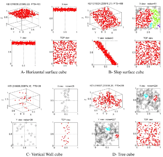
In Figure 3, a considerable distance reduction between the points is visible when the 300
irrelevant dimensions Y and X have been removed from the corresponding views. Although 301
removing dimensions is useful in the case of the X-view and Y-view, the same approach is not 302
applicable in the case of the Z-view (Top). As shown in Figure 3, there are a lot of holes between 303
the points from the TOP-view. For this reason, this view is not considered in the approach presented 304 herein. 305 306 307 308 309
Figure 3. Some of the representative cubes. 310
Figure 3 also illustrates some of the representative cubes of the DSM. Figure 3-A shows a 311
prismatic cube with the key identification KEY(316030,233982,22) and 453 points. The cube 312
consists of a horizontal surface, which represents a subspace of a building roof with a height equal 313
to 22 m. Within the cube’s prismatic shape, there are some holes between the points. However, 314
when the Y-dimension and the X-dimension are removed in the X-view and Y-view respectively, 315
clusters are readily visible. This is to say, the X-view is the projection to the XZ plane, and Y-view 316
is the projection to the YZ plane. In this case, the noise in the two views is equal to zero, so that this 317
cube is classified as a dense cube. Noise points are presented in the Figure as small circles. The 318
cube in Figure 3-B is a sloped building roof. This cube is also classified as dense, although the 319
noise in the X-view is significant (noise = 113 points), because the noise point number in the Y-320
view is 0. The cube in Figure 3-C represents a vertical building wall. This cube is classified as 321
sparse, because neither of the two views forms a cluster. The percentage of the noise points in the 322
two views exceeds that of the maxNoise. As previously noted by Jochem et al. (2006) the relative 323
position of the aircraft to the building wall and the large incidence angles often limits point 324
acquisition on these vertical surface, which could affect negatively the results, because the cubes 325
from vertical walls are formed with relatively low point densities. 326
Notably, a general move to higher point densities and new means of flight path planning to 327
maximize vertical data capture (e.g., Hinks et al. 2009) should help to mitigate this problem. 328
Furthermore, this limitation when it generates a gap could be used to identify a separation between 329
the ground surface and the building roofs, further facilitating roof classification, localization, and 330
then the extraction. Figure 3-D shows a cube that represents vegetation or other undesirable points. 331
No cluster emerges in either of the two views. So this cube is classified as a sparse cube, because 332
the percentage of noise in the both views is greater than the allowed percentage. 333
334
Step-3: Clustering interesting cubes
335
Once the two cube types are generated, the sparse cubes are removed. The remaining dense cubes 336
are grouped into clusters, with each cluster representing the outline of an object. To do that, the 337
Neighbour Adjacent Cube Algorithm is applied. In that algorithm, two adjacent cubes belong to the 338
same object. This algorithm starts from the highest cube in the dataset and moves downwards 339
towards the lowest one. As previously mentioned, because vertical walls cubes are not classified as 340
dense cubes, empty spaces form between the roof building cubes and the ground cubes. Once the 341
highest object is segregated, the algorithm next segregates the highest remaining object in the DSM. 342
This continues, until all objects are segregated from the DSM. Notably, although the algorithm 343
always starts with the highest object, this does not require a height calculation of each object, only 344
determination as to which cube has the highest Z coordinate. This is an improvement over other 345
related works [e.g., Zhang et al. (2006), Abdullah at el. (2014), and Aljumaily at el. (2015)] where 346
object height calculation was needed prior to extraction. 347
At the end of the classification and then the extraction processes, the DSM dataset being 348
processed will be empty, because all of its cubes will have been segregated and moved 349
automatically to the corresponding files where each file represents a cluster. A limitation of this 350
approach is that if two buildings are joined together (see Figure 4) [e.g., terraced housing], the 351
approach recognizes them as a single object. This is a well-known problem for many techniques 352
attempting individual building extraction, as reported by Truong-Hong and Laefer (2015). 353
354
355
Figure 4. An object with multiples adjacent buildings. 356
EXPERIMENTS AND RESULTS
357
The clustering approach presented in Section 3 is evaluated herein on an architecturally dense and 358
complex portion of Dublin, Ireland with the aforementioned 225pts/m2 data. Within the 1 km2 study
359
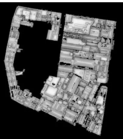
area, there are 9 tiles from the DSM (see Figure 5). The DSM preparation included several steps 360
that are outside of the scope of this work, including flight path planning, as well as data collection, 361
registration, and filtering (as described in Truong-Hong, 2011). 362
364
Figure 5. DSM of the study area generated herein 365
The proposed approach depends on the point cloud density. This DSM contained 366
225,793,264 points according to the first step of the approach (Step-1). These points were mapped 367
to 3,248,520 cubes resulting in an average of 70 points per cube with a standard deviation of 105.5 368
points. Their distribution is shown in Figure 6, where the x-axis shows the density divided into 10 369
point intervals (e.g., the first represents cubes containing 1-10 points). In the last interval, there was 370
only 1 cube, which contained 666 points, which was the densest in the data set. The peak of the 371
histogram represents that 3.95% of the points of the DSM. Those cubes contained 241-250 points. 372
373
Figure 6. Distribution percentages of the DSM original 374
To quantitatively evaluate the approach’s outputs, the following metrics were used: (1) 375
measurements of correctness, (2) completeness and (3) fitness measure (F-measure). Many 376
researchers use the terms precision and correctness interchangeably. The same is true for the terms 377
recall and completeness. In this paper the terms correctness and completeness will be used to be 378
consistent with the authors’ previously published work (i.e. Aljumaily et al. 2015). Normally, these 379
measures are calculated by taking the difference between the classified objects and the reference 380
objects (Maurya et al. 2012). According to Rutzinger et al. (2009), the correctness evaluates the 381
exactness of the approach and is a ratio of the relevant points of a classified object to the total 382
number of points of the referenced objects (see eqn 6). A point was considered relevant, if the 383
approach classified it correctly, with respect to the corresponding reference object. The 384
completeness is the ratio of the classified relevant points to the total number of points in the 385
referenced objects (see eqn 7). The F-measure or fitness evaluates the overall quality (see eqn 8). 386
These metrics are calculated using terms such as True Positives (TP), False Positives (FP), and 387
False Negatives (FN). TP are the points correctly included into this object, FP are the points 388
incorrectly included into this object, and FN are the points mistakenly excluded for this object. 389 correctness FP TP TP + = ……… (eqn 6) 390 completeness FN TP TP + = ……….. (eqn 7) 391 F-measure FN FP TP TP + + = ………. (eqn 8) 392 393
As mentioned in the previous section, in order to apply the DBSCAN algorithm several 394
parameters (i.e. Eps and MinPts) must be set. Because these parameters depend on the features of 395
the dataset, the accuracy of the resulting clustering is directly depending on the user’s choice of 396
parameters (Zhou et. al. 2012). For this reason, an empirical study was undertaken on the selected 397
DSM to optimize these parameters for optimal clustering results. In this study, initial values for 398
each parameters were assigned. These were then increased incrementally and individually until a 399
degradation of the results was observed. A global optimisation was not, however, undertaken. The 400
initial values of Eps and MinPts were selected as 0.1m and 10 points, respectively based on the 401
belief that 0.1 m would be a reasonable distance between two points in a DSM to form a cluster, 402
and a cluster with less than 10 points having insufficient information for meaningful post-403
processing activities. The values of Eps and MinPts were increased by 0.05m and 10 points, 404
respectively. In addition, maxNoise was used as a third parameter to distinguish between a 405
classification of dense and sparse. In the same way an initial value of (maxNoise < 10) was selected 406
as the division between dense and sparse cubes. This is to say, if the percentage of the noise in a 407
cube was less than or equal to 10%, then this cube was considered as a dense cube but otherwise as 408
sparse cube. An initial setting of 0% only resulted in a clustering of 7% of the data, thus the selected 409
lowerbound threshold was 10%. The incremental value of maxNoise was established as 10% for 410
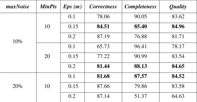
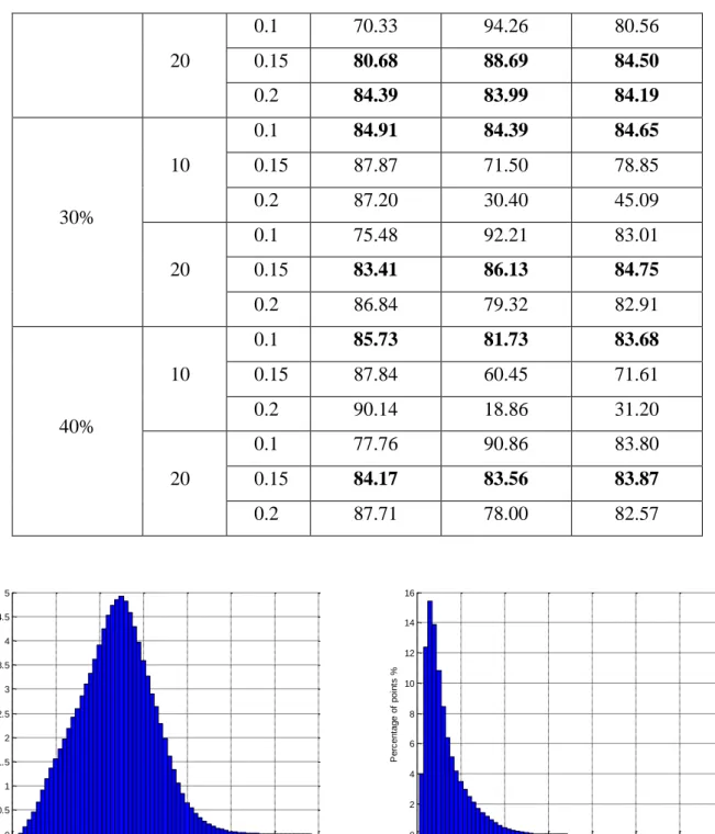
each iteration (i.e., 10%, 20%, 30%, etc). The most significant results of this study are shown in 411
Table 1, where the bolded values represent the most interesting results of the approach. As shown in 412
Table 1, many results are similar often achieving around 85% correctness despite being derived 413
from different thresholds; with the remaining 15% likely to have been lost because of the 414
complexity of the architecture of the building and the difficulties related to the manual extraction of 415
the reference objects. Clearly, a further development step is needed in which a formal optimization 416
process is undertaken. With this caveat understood, a single case will be further investigated below. 417
Due to space limitations only one set of results is further presented (Eps = 0.1m, MinPts=10, and 418
maxNoise<30%). Those achieved nearly 85% in all three categories: correctness = 84.91, 419
completeness = 84.39, quality = 84.65 (Table 1). 420
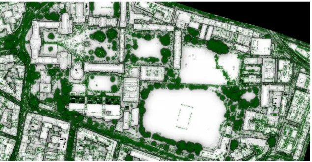
Figure 7 illustrates the analysis of the clustering results, where two sets of points can be 421
distinguished. The first are the points of the dense cubes (Figure 7-A) representing approximately 422
80% of the DSM across 30% of the cubes, with an average density of approximately 185 pts/cube 423
and a standard deviation of 85.0. They display a normal distribution. The second are the points of 424
the sparse cubes (Figure 7-b) representing approximately 20% of the DSM across 70% of the cubes 425
with an average density of approximately 20 pts/cube and a standard deviation of 44.6 displaying a 426
normal distribution. In these figures, there is a separation between cubes with high point density and 427
those with low point density. Those with a density of 250 points/cube are definitely dense 428
categorization and those with a density of less than 100 points per cube definitively sparse. Looking 429
at Figure 7, most of the cubes that contained between 100 and 250 points per cube were classified 430
ultimately by the proposed approach as dense cubes. 431
432
Table 1. The most significant results of the empirical study. 433
434
maxNoise MinPts Eps (m) Correctness Completeness Quality
10% 10 0.1 78.06 90.05 83.62 0.15 84.51 85.40 84.96 0.2 87.19 76.88 81.71 20 0.1 65.73 96.41 78.17 0.15 77.22 90.99 83.54 0.2 81.44 88.13 84.65 20% 10 0.1 81.68 87.57 84.52 0.15 87.66 79.86 83.58 0.2 87.14 51.37 64.63
20 0.1 70.33 94.26 80.56 0.15 80.68 88.69 84.50 0.2 84.39 83.99 84.19 30% 10 0.1 84.91 84.39 84.65 0.15 87.87 71.50 78.85 0.2 87.20 30.40 45.09 20 0.1 75.48 92.21 83.01 0.15 83.41 86.13 84.75 0.2 86.84 79.32 82.91 40% 10 0.1 85.73 81.73 83.68 0.15 87.84 60.45 71.61 0.2 90.14 18.86 31.20 20 0.1 77.76 90.86 83.80 0.15 84.17 83.56 83.87 0.2 87.71 78.00 82.57 435
A- Dense Cubes B- Sparse Cubes
Figure 7. Clustering classification results for Eps = 0.1m, MinPts=10, and maxNoise<30% 436
Figure 8 shows a comparison study between the reference objects and those automatically 437
classified objects by the approach proposed herein. First, the reference objects (Figure 8-A) were 438
manually extracted from the original DSM. In total, there were 106 building groups and 1 ground 439
surface. This was done using the visualization tool CloudCompare (Compare, 2015); most features 440
within the study area (e.g., buildings, roads, trees) were easily distinguishable with the naked eye. 441
CloudCompare provides editing features such as DSM segmentation. Each colour in Figure (8-B) 442
represents a classified object. Giving a colour to an object means that the object was defined, and all 443 0 100 200 300 400 500 600 700 0 0.5 1 1.5 2 2.5 3 3.5 4 4.5 5
Density (number of points/cube)
P e rc e n ta g e o f p o in ts % 0 100 200 300 400 500 600 700 0 2 4 6 8 10 12 14 16
Density (number of points/cube)
P e rc e n ta g e o f p o in ts %
the relevant information about it (e.g., coordinates, dimensions, outlines) was harvested to enable 444
simple extraction of the whole object from the original DSM. 445
For simplicity, the previous parameters (TP, FP, and FN) were calculated only considering 446
the cube level. This is to say, all the cubes that were included in both DSMs (Figure 8-A and 8-B) 447
were considered as TP, if all the cubes that were included in the DSM are classified correctly as 448
objects (Figure 8-B). They were FP if they classified an object that did not appear as a reference 449
objects (Figure 8-A). Finally, all cubes that were included in the DSM as reference objects (Figure 450
8-A) but not classified objects (Figure 8-B) were considered as FN. The same approach was taken 451
with respect to the classification of the ground surface (Figure 8-C and 8-D). 452
A- DSM of the Reference Objects B- DSM of the Classified Objects
C- The reference of the ground surface D- The cluster of the classified ground surface Figure 8. Quantitative evaluate of the approach’s outputs for Eps = 0.1m, MinPts=10, and 453
maxNoise<30%. 454
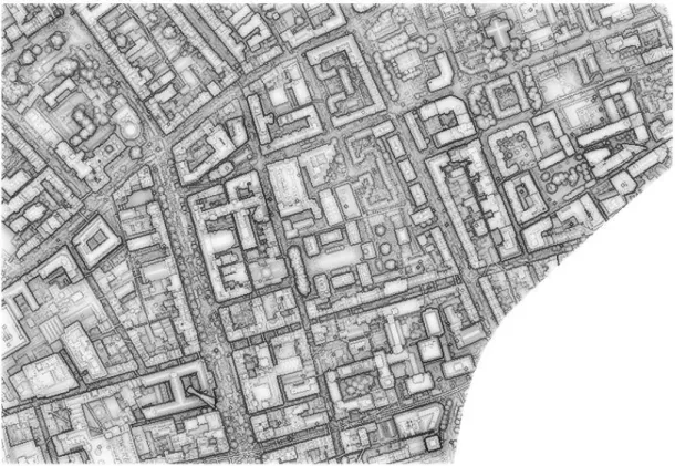
As visible in Figure 9, the approach was able to classify the heavy vegetation and other 455
obstructions in the DSM and able to segregate fully automatically the outlines of building groups 456
from the roads and the ground surface. The approach was also very successful for classifying 457
building groups with complicated roof geometries and those with multiple sections of varying 458 heights. 459 460 461
Figure 9. Vegetation detection by the proposed approach. 462
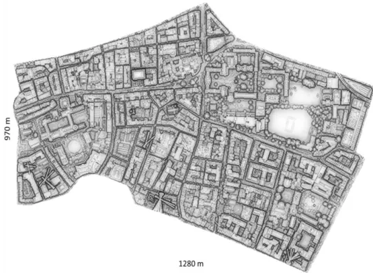
In order to validate the results of the proposed approach, a new DSM of approximately 1 463
km2 was considered (Figure 10). This new data set was selected also from an architecturally dense
464
and complex portion of Dublin, Ireland. The new data set contained 158,890,014 points. These 465
points were mapped to 2,150,979 cubes. This DSM was selected, because it is more complicated 466
than the first one, where many small objects with vegetation and other obstacles were included. 467
469
Figure 10. DSM of the second study area generated herein 470
In the validation of the second study area the same thresholds were selected (Eps=0.1m, 471
MinPts=10, and maxNoise < 30%. The results of the extraction quality were slightly poorer 472
(correctness=80.02%, completeness=78.01%, and overall quality = 79.44%). The difference 473
between the qualities of the both study areas is in part an outgrowth of the difficulty of manual 474
extraction of the second study area where errors may be introduced. In Figure 11, the DSM of the 475
classified objects and the referenced objects are shown. 476
A- DSM of the Reference Objects B- DSM of the Classified Objects Figure 11. Quantitative evaluate of the approach’s outputs of the second case study. 477
The computational efficiency and scalability of the approach needs to be demonstrated with 478
respect to the execution time required for each step of the proposed approach. All the experiments 479
were conducted on a PC with an Intel Core i7 CPU 2.40GHz, 12GB Memory. Regarding to Step-1 480
(MapReduce Step) the experiment was done using a single node of a Hadoop installation. The 481
results of execution time are shown in Figure 12. In this figure, the experiments were done by 482
selecting three different cube dimensions (0.5m, 1.0m, and 2.0m) of the same DSM (Figure 5). 483
Notably, the execution time using cubes with dimensions of 0.5m were very similar to those using 484
dimensions of 1.0m. A value of d of 1.0m is recommended, because when the cube dimension is 485
small and there are many cubes of low density with complex architecture, the original cluster will 486
unnecessarily be divided into smaller clusters and this will reduce the quality of the clustering. If a 487
big cube dimension such as 2.0m is selected, other problems arise. The main problem is that when 488
the cube dimension is large, a cube may contain parts of different objects including vegetation, 489
which results in their ultimate misclassification. In addition, big cube dimensions mean that there 490
are a high number of points to be processed within each cube. Consequently, extensive execution 491
time will be need in the next steps. 492
493
Figure 12. Execution time of the MapReduce step with three different dimensions cubes 494
Notably, the execution time of the MapReduce step can be improved easily by adding more 495
nodes as is common for a Big Data platform cluster (Xu et al. 2015). According to the result 496
showed in Wang et al. (2010) using a cluster of 8 nodes a MapReduce based spatial system 497
consumes approximately 0.24% of the initial time. 498
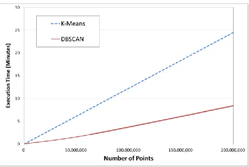
500
Figure 13. Comparison between the proposed execution time for DBSCAN versus K-Means time 501
Regarding to the second step (Recognizing interesting subspaces), as mentioned in the 502
related works section, the DBSCAN is considered a classic clustering algorithm based on density. 503
The complexity of this algorithm is O(n*logn), and it is robust towards outlier detection (Noise) 504
(Xu et al. 2015). Other classic algorithm such as K-means is not built for outliers’ detection 505
purpose. However, in this section in order to ensure the validity of the performance of the DBSCAN 506
algorithm, a comparison between DBSCAN and the Means has been done. But firstly, the K-507
Means algorithm has been adapted for our approach, i.e., improving K-Means in order to detect 508
outliers according to the approach presented into (McCaffrey 2013). The result of the comparison is 509
shown in Figure 13, where it is clearly shown that the DBSCAN algorithm provides better 510
performance than the K-Means algorithm. For example, in order to cluster 200,000,000 points the 511
DBSCAN needs no more 9 minutes while the K-Means needs approximately 25 minutes. The 512
difference likely stems from the fact that DBSCAN was built to detect outliers, while the K-Means 513
was built for space partitioning, with outlier detection and removal as added components (e.g., 514
Hautamäki, et. al. 2005). 515
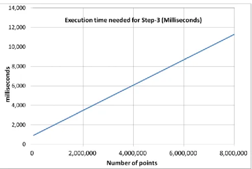
The time for Step-3 (Clustering interesting cubes) of the approach is insignificant when 516
compared with the time needed for the first two phases. The execution time of Step-3 (see Figure 517
14) depends on the size of the object extracted. The object classification time depends on the 518
number of affiliated and adjacent points. For example, in the case presented herein, each of the 519
classified clusters (73%) had less than 1,000,000 points. So, to cluster interesting cubes of an object 520
with 1 million points, this Step-3 needed approximately 2,000 milliseconds (see Figure 14). 521
523
Figure 14. Execution time of the clustering interesting cubes step of the approach 524
CONCLUSIONS
525
Most current solutions for building classification and extraction from point cloud data are hard to 526
scale with respect to the forward trajectory of data densities levels. To address this in the context of 527
object classification, localization and extraction, this paper presents the implementation of a fully 528
automatic and significantly more scalable approach than otherwise available to support clustering of 529
LiDAR data in a Big Data context. The approach was tested with two study areas on approximately 530
2 km2 where more than 200 objects in the DSM were automatically detected at an average
531
classification quality level of 85% including those with complicated roof geometries and those with 532
multiple sections of varying heights. The approach was able to classify the heavy vegetation and 533
other obstructions in the DSM and was able to segregate fully and automatically the outlines of 534
buildings from the roads and ground surface. 535
536
According to the obtained results, this paper presents the viability to use a clustering 537
algorithm (DBSCAN) based on point density for the objects extraction from a DSM. This kind of 538
clustering is suitable for data with arbitrary shape and is able to discard noise or outliers (in this 539
case, points that do not belong to a building or road). While the current implementation DBSCAN 540
algorithm has the drawbacks of requiring a high memory capacity with big volume data, the Big 541
Data framework where the approach is being developed will largely alleviates this problem. In the 542
ongoing work, the issue of a global optimization strategy for automated parameter selection will 543 also be considered. 544 545 546 ACKNOWLEDGMENTS 547
This work was in part supported with funds from the European Research Council Project 307836. 548
REFERENCES
550
Abdullah, S., Awrangjeb, M., and Lu, G. Automatic segmentation of LiDAR point cloud data at 551
difference height levels for 3D building extraction. IEEE International conference on
552
Multimedia and Expo workshops (ICMEW) (Chengdu, 2014) (pages 1-6). 553
Aggarwal, C. C., & Reddy, C. K. (Eds.). (2013). Data clustering: algorithms and applications. 554
CRC Press. 555
Aljumaily, H., Laefer, D. F., & Cuadra, D. (2015). Big-Data Approach for Three-Dimensional 556
Building Extraction from Aerial Laser Scanning. Journal of Computing in Civil Engineering, 557
30(3), 04015049. 558
Awrangjeb, M., Zhang, C., & Fraser, C. S. (2013). Automatic extraction of building roofs using 559
LiDAR data and multispectral imagery. ISPRS Journal of Photogrammetry and Remote
560
Sensing, Volume 83, September 2013, Pages 1-18. 561
Compare, C. (2015). 3D point cloud and mesh processing software Open Source Project. License: 562
GNU GPL (General Public Licence), Version: 2.6, http://www.danielgm.net/cc 563
Chang, J. W. (2005, September). A new cell-based clustering method for high-dimensional data 564
mining applications. In International Conference on Knowledge-Based and Intelligent
565
Information and Engineering Systems (pp. 391-397). Springer Berlin Heidelberg. 566
Chang, J. W., & Jin, D. S. (2002, March). A new cell-based clustering method for large, high-567
dimensional data in data mining applications. In Proceedings of the 2002 ACM symposium on
568
Applied computing (pp. 503-507). ACM. 569
Chakrawarty, L., & Gupta, P. (2014) Applying SR-Tree technique in DBSCAN clustering 570
algorithm. International Journal of Application or Innovation in Engineering & Management. 571
Volume 3, Issue 1, January 2014, pages 207-210. 572
Chen, Y., Crawford, M., & Ghosh, J. (2006, July). Improved nonlinear manifold learning for land 573
cover classification via intelligent landmark selection. In 2006 IEEE International Symposium
574
on Geoscience and Remote Sensing (pp. 545-548). IEEE. 575
Darong, H., & Peng, W. (2012). Grid-based DBSCAN algorithm with referential parameters. 576
Physics Procedia, 24, 1166-1170. 577
Ester, M., Kriegel, H. P., Sander, J., & Xu, X. (1996, August). A density-based algorithm for 578
discovering clusters in large spatial databases with noise. In Kdd (Vol. 96, No. 34, pp. 226-231). 579
Fu, X., Hu, S., & Wang, Y. (2014). Research of parallel DBSCAN clustering algorithm based on 580
MapReduce. International Journal of Database Theory and Application, 7(3), 41-48. 581
Hautamäki, V., Cherednichenko, S., Kärkkäinen, I., Kinnunen, T., & Fränti, P. (2005, June). 582
Improving k-means by outlier removal. In Scandinavian Conference on Image Analysis (pp. 583
978-987). Springer Berlin Heidelberg. 584
Jain, A. K. (2010). Data clustering: 50 years beyond K-means. Pattern recognition letters, 31(8), 585
651-666. 586
Jochem, A., Höfle, B., & Rutzinger, M. (2011). Extraction of vertical walls from mobile laser 587
scanning data for solar potential assessment. Remote sensing, 3(4), 650-667. 588
Jochem, A., Höfle, B., Wichmann, V., Rutzinger, M., Zipf, (2012) A. Area-wide roof plane 589
segmentation in airborne LiDAR point clouds. Comput. Environ. Urban Syst. 2012, 36, 54-64. 590
Kailing, K., Kriegel, H. P., & Kröger, P. (2004, April). Density-connected subspace clustering for 591
high-dimensional data. In Proc. SDM (Vol. 4). Pages 246-256 592
Kurasova, O., Marcinkevicius, V., Medvedev, V., Rapecka, A., & Stefanovic, P. (2014, November). 593
Strategies for big data clustering. In 2014 IEEE 26th International Conference on Tools with
594
Artificial Intelligence (pp. 740-747). IEEE. 595
Lee, I., Cai, G., & Lee, K. (2014). Exploration of geo-tagged photos through data mining 596
approaches. Expert Systems with Applications, 41(2), 397-405. 597
Li, Y., Wu, H., An, R., Xu, H., He, Q., & Xu, J. (2013). An improved building boundary extraction 598
algorithm based on fusion of optical imagery and LiDAR data. Optik-International Journal for
599
Light and Electron Optics, 124(22), 5357-5362. 600
Maurya, R., Gupta, P. R., Shukla, A. S., & Sharma, M. K. (2012, March). Building extraction from 601
very high resolution multispectral images using NDVI based segmentation and morphological 602
operators. In Advances in Engineering, Science and Management (ICAESM), 2012 International
603
Conference on (pp. 577-581). IEEE. 604
McCaffrey J. (February 2013) Data Clustering - Detecting Abnormal Data Using k-Means 605
Clustering. In The Microsoft journal for developers.
https://msdn.microsoft.com/en-606
us/magazine/jj891054.aspx
607
Parsons, L., Haque, E., & Liu, H. (2004). Subspace clustering for high dimensional data: a review. 608
ACM SIGKDD Explorations Newsletter, 6(1), 90-105. 609
Rottensteiner, F., Trinder, J., Clode, S., & Kubik, K. (2004). Fusing airborne laser scanner data and 610
aerial imagery for the automatic extraction of buildings in densely built-up areas. International
611
Archives of Photogrammetry and Remote Sensing, 35(B3), 512-517. 612
Rutzinger, M., Rottensteiner, F., & Pfeifer, N. (2009). A comparison of evaluation techniques for 613
building extraction from airborne laser scanning. IEEE Journal of Selected Topics in Applied
614
Earth Observations and Remote Sensing, 2(1), 11-20. 615
Slatton, K.C., and Carter,W.E.,2008,A Primer for Airborne LiDAR. The National Center for 616
Airborne Laser Mapping (NCALM)
617
http://ncalm.cive.uh.edu/sites/ncalm.cive.uh.edu/files/files/publications/reports/LidarPrimer-618
Final02.pdf
Truong-Hong, L. (2011). Automatic Generation of Solid Models of Building Facades from LiDAR 620
Data for Computational Modelling. , Ph. D. Thesis, University College Dublin 621
Truong‐Hong, L., Laefer, D. F., Hinks, T., & Carr, H. (2013). Combining an angle criterion with 622
voxelization and the flying voxel method in reconstructing building models from LiDAR data. 623
Computer‐Aided Civil and Infrastructure Engineering, 28(2), 112-129. 624
Truong-Hong, L., Laefer, D. (2015). “Quantitative Evaluation Strategies for Urban 3D Model 625
Generation from Remote Sensing Data.” Computers and Graphics, Elsevier, 626
doi.org/10.1016/j.cag.2015.03.001i. 627
UCD Digital Library, (2007) http://dx.doi.org/10.7925/DRS1.UCDLIB_30462
628
Vo, A. V., Truong-Hong, L., Laefer, D. F., & Bertolotto, M. (2015). Octree-based region growing 629
for point cloud segmentation. ISPRS Journal of Photogrammetry and Remote Sensing, 104, 88-630
100. 631
Wang et al. 2010, Dec. Accelerating spatial data processing with mapreduce. Parallel & Distrib. 632
Sys. IEEE pages 229-236. 633
Wang, C., Hu, X., Ji, M., & Li, T. (2013). An Automated 3D Approach for Buildings 634
Reconstruction from Airborne Laser Scanning Data. In Geo-Informatics in Resource
635
Management and Sustainable Ecosystem (pp. 704-712). Springer Berlin Heidelberg. 636
Wu, Y. P., Guo, J. J., & Zhang, X. J. (2007, August). A linear dbscan algorithm based on lsh. In 637
Machine Learning and Cybernetics, 2007 International Conference on (Vol. 5, pp. 2608-2614). 638
IEEE. 639
Xu, D., & Tian, Y. (2015). A comprehensive survey of clustering algorithms. Annals of Data 640
Science, 2(2), 165-193. 641
Xu, G., Yu, W., Chen, Z., Zhang, H., Moulema, P., Fu, X., & Lu, C. (2015). A cloud computing 642
based system for cyber security management. International Journal of Parallel, Emergent and
643
Distributed Systems, 30(1), 29-45. 644
Zhang et al. 2009, Aug. Spatial queries evaluation with mapreduce. Grid & Coop Comp 2009, 287-645
92. IEEE 646
Zhang, K., Yan, J., & Chen, S. C. (2006). Automatic construction of building footprints from 647
airborne LíDAR data. IEEE Transactions on Geoscience and Remote Sensing, , 44(9), pages 648
2523-2533. 649
Zhou, H., Wang, P., & Li, H. (2012). Research on adaptive parameters determination in DBSCAN 650
algorithm. Journal of Information & Computational Science, 9(7), 1967-1973. 651
Zhou, X., Xu, C., & Kimmons, B. (2015). Detecting tourism destinations using scalable geospatial 652
analysis based on cloud computing platform. Computers, Environment and Urban Systems, 54, 653
144-153. 654