Concepts for In-memory Event Tracing: Runtime Event Reduction with Hierarchical Memory Buffers

(1)

T

ECHNISCHE

U

NIVERSITÄT

DRESDEN

F

AKULTÄT

I

NFORMATIK

Dissertation

zur Erlangung des akademischen Grades Doktoringenieur (Dr.-Ing.)

Concepts for In-memory Event Tracing

Runtime Event Reduction with Hierarchical Memory Buffers

Michael Wagner

geboren am 18. Mai 1984 in Bad Schlema

Gutachter: Prof. Dr. Wolfgang E. Nagel Technische Universität Dresden Prof. Dr. Felix Wolf

Technische Universität Darmstadt

(2)

(3)

Abstract

This thesis contributes to the field of performance analysis in High Performance Computing with new concepts for in-memory event tracing.

Event tracing records runtime events of an application and stores each with a precise time stamp and further relevant metrics. The high resolution and detailed information allows an in-depth analysis of the dynamic program behavior, interactions in parallel applications, and potential performance issues. For long-running and large-scale parallel applications, event-based tracing faces three challenges, yet unsolved: the number of resulting trace files limits scalability, the huge amounts of collected data over-whelm file systems and analysis capabilities, and the measurement bias, in particular, due to intermediate memory buffer flushes prevents a correct analysis.

This thesis proposes concepts for an in-memory event tracing workflow. These concepts include new enhanced encoding techniques to increase memory efficiency and novel strategies for runtime event re-duction to dynamically adapt trace size during runtime. An in-memory event tracing workflow based on these concepts meets all three challenges: First, it not only overcomes the scalability limitations due to the number of resulting trace files but eliminates the overhead of file system interaction altogether. Second, the enhanced encoding techniques and event reduction lead to remarkable smaller trace sizes. Finally, an in-memory event tracing workflow completely avoids intermediate memory buffer flushes, which minimizes measurement bias and allows a meaningful performance analysis.

The concepts further include theHierarchical Memory Bufferdata structure, which incorporates a multi-dimensional, hierarchical ordering of events by common metrics, such as time stamp, calling context, event class, and function call duration. This hierarchical ordering allows a low-overhead event encoding, event reduction and event filtering, as well as new hierarchy-aided analysis requests.

An experimental evaluation based on real-life applications and a detailed case study underline the capa-bilities of the concepts presented in this thesis. The new enhanced encoding techniques reduce memory allocation during runtime by a factor of 3.3 to 7.2, while at the same do not introduce any additional overhead. Furthermore, the combined concepts including the enhanced encoding techniques, event re-duction, and a new filter based on function duration within the Hierarchical Memory Buffer remarkably reduce the resulting trace size up to three orders of magnitude and keep an entire measurement within a single fixed-size memory buffer, while still providing a coarse but meaningful analysis of the application. This thesis includes a discussion of the state-of-the-art and related work, a detailed presentation of the enhanced encoding techniques, the event reduction strategies, the Hierarchical Memory Buffer data struc-ture, and a extensive experimental evaluation of all concepts.

(4)

(5)

I

1 Introduction

It is beneath the dignity of excellent men to waste their time in calculation when any peasant could do the work just as accurately with the aid of a machine.

GOTTFRIEDWILHELMLEIBNIZ

When Gottfried Wilhelm Leibniz presented theStepped Reckoner, the first calculation machine, to the Royal Society of London in 1673 he paved the way to today’s computers. While his and all following calculation machines of the next two centuries did not use electronics but were the product of precise engineering, he already constituted his machine supra hominem – superior to humans – since it out-performed humans in speed, as well as accuracy, for large calculations. With the advent of electronic computers, first based on electromechanical relays and later on vacuum tubes and transistors, the ca-pabilities and performance of machine-aided computing began to grow rapidly. Nowadays, computing devices are omnipresent and an integral part of many aspects of life. Particularly in science and research, computer-aided simulation has become indispensable and is considered the third cornerstone of scientific methodology besides theory and experiment.

Beyond everyday computing devices, High Performance Computing (HPC) systems provide enormous computational resources to support large-scale simulations in leading-edge scientific research such as the Human Brain project [MML+11], climate and weather prediction, or DNA and cancer research. Today, High Performance Computing typically includes a large number of processing elements working jointly on a computationally intensive problem. For the next milestone, exa-scale supercomputers capable of

O(1018)floating point operations per second, this approach is very likely to persist. For the foreseeable future Moore’s law [Moo65] is expected to endure, however, limitations in clock frequency, instruction level parallelism, and energy density drive the further increase in the number of processing elements. In addition, supercomputing hardware is strongly influenced by economy-driven developments in the off-the-shelf market, as shown, for instance, by the integration of accelerators from graphic cards. The history of TOP500 [Top14] systems shows that not all system characteristics improve at the same speed as computing power. Critical properties are main memory bandwidth and latency, the amount of memory per core, I/O capabilities, as well as energy consumption [BBC+08]. Consequently, supercomputers targeting the exa-scale barrier are likely to be specialized solutions with tremendous computational power but also many constraints that have a considerable impact on efficient software development.

Parallel software that scales to the exa-scale level implies the identification, distribution, and synchro-nization of millions of subproblems that can be computed autonomously. Any computationally intensive problem requires the decomposition in subtasks, whose partial results must be accumulated efficiently to the overall solution. Writing software for systems of this scale is demanding and involves hybrid and new programming models, accelerated computing, and energy considerations. Hence, appropriate supporting tools, such as debuggers and performance analyzers, are inevitable to develop applications that utilize the enormous capabilities of current and future HPC systems.

(10)

Performance analysis tools assist developers not only in identifying performance issues in their applica-tions but also in understanding their behavior on complex and heterogeneous systems. Such tools gather information about the behavior of an application during runtime by either recording runtime events or by periodically sampling its current state. While sampling approaches rely on their sampling frequency to gain information about an application, event-based monitoring tools record information if specific predefined events occur, for instance, entering and leaving a function.

Information gathered from samples or events can be aggregated to summarized information about differ-ent performance metrics (profiling) or stored individually by keeping the precise time stamp and further specific metrics for each event (tracing). Profiling with its nature of summarization decreases the amount of data that needs to be stored during runtime. However, profiles may lack critical information and hide dynamically occurring effects. In contrast, event tracing records each event of a parallel application in detail and allows an exact reconstruction of the application behavior. Thus, it enables capturing the dy-namic interaction between thousands of concurrent processing elements and the identification of outliers from the regular behavior. Such detail comes with the cost that event-based tracing frequently results in huge data volumes even though single events are rather small. In fact, the large amount of collected data, in particular, for massively parallel or long running applications is one of the most urgent challenges for event-based monitoring tools.

In both dimensions event tracing is already pushing against the limits of today’s and, most likely, also tomorrow’s systems. Since the collected data is usually stored in one file per processing element, the number of resulting trace files is increasing with the number of recorded processing elements. While HPC parallel file systems are highly optimized for data throughput, the simultaneous creation of hun-dreds of thousands or even millions of event tracing files overwhelms any parallel file system and the aggregated size of the resulting trace files quickly swallows up storage capacities. Next to that, the recorded event data is typically buffered before it is written to the file system to reduce expensive file system interactions. Whenever such an internal memory buffer is exhausted, the content is transferred to the file system; usually in an unsynchronized fashion. Such uncoordinated intermediate memory buffer flushes during a measurement introduce extensive bias and lead to a falsification of the recorded program behavior. Much like system noise this effect is increasing with higher scales.

Another way to circumvent these constraints is an in-memory event tracing workflowthat completely omits file system interaction. Keeping recorded event data in main memory for the complete workflow would not only bypass the limitations in the number of file handles, moreover, it would eliminate the overhead of file creation, writing and reading altogether. In addition, an in-memory workflow would exclude the bias caused by non-synchronous intermediate memory buffer flushes during a measurement run. Furthermore, such a workflow allows entirely new features in event tracing, such as an event-based online performance analysis workflow.

But there is one catch. Keeping event data in main memory for a complete measurement requires that recorded data fits into a single memory buffer of an event tracing library. Unfortunately, measurement runs may collect hundreds of megabytes up to gigabytes of data per processing element. To make things worse, the part of the main memory left to store the data is rather small, since most applications utilize main memory intensively. This thesis is dedicated to the challenge of fitting an entire measurement of arbitrary length and scale into a single fixed-sized memory buffer for each processing element and, therefore, setting the premise for an in-memory event tracing workflow.

(11)

3

Contribution of this Thesis

The contributions of this thesis are novel concepts to enable an in-memory event tracing workflow. These concepts are divided in two central parts:

Enhanced encoding techniquesandstrategies for event reductionthat dynamically adapt trace size during

runtime to the given memory allocation form the first central part of the contributions of this thesis. The combination of both allows keeping the data of an entire measurement within a single fixed-sized memory buffer and, therefore, enable an in-memory event tracing workflow. First, such an in-memory tracing workflow not only bypasses the limitations of current parallel file systems but eliminates the overhead of file system interaction altogether. Second, the enhanced encoding techniques and event reduction result in remarkably smaller trace sizes. Furthermore, the in-memory workflow completely avoids intermediate memory buffer flushes and, therefore, minimizes measurement bias, which allows a feasible tracing of long running applications.

TheHierarchical Memory Bufferis the second central contribution of this thesis. The Hierarchical

Mem-ory Buffer is a new data structure that uses hierarchy information, such as calling depth or event class, to presort events according to these hierarchy attributes. It allows performing the aforementioned event reduction operations with minimal overhead. Furthermore, such a hierarchy-based event representation allows new event filter operations, unfeasible with a traditional flat, continuous memory buffer layout. Such a new filter method is a filtering based on the duration of code regions, which eliminates all short-running functions while keeping outliers important for performance analysis. In addition, several typical analysis requests can benefit from a hierarchy-aided traversal of recorded event data.

Organisation of this thesis

The next chapter, State-of-the-art in Event-based Performance Analysis, provides an overview of the state-of-the-art in event-based performance analysis and performance analysis tools. Furthermore, tools for event-based trace recording and analysis are discussed in more detail. On the basis of three current challenges the chapter introduces related work and connects the contributions of this thesis.

The chapter onConcepts for In-memory Event Tracingspecifies prerequisites for an in-memory event tracing workflow and defines three key steps to keep an entire measurement within a single fixed-size memory buffer. These three key steps are selection and filtering, enhanced encoding, and event reduction. New methods for each step are presented.

The chapterThe Hierarchical Memory Bufferintroduces the Hierarchical Memory Buffer, a data structure that allows to perform event reduction operations with minimal overhead. It examines algorithms for the construction of this data structure, as well as the application of the event reduction strategies and typical analysis techniques. Furthermore, the computational complexity of all algorithms is discussed.

The chapterEvaluation and Case Studypresents an evaluation of the enhanced encoding techniques and the Hierarchical Memory Buffer data structure including its capabilities to support the event reduction strategies. In addition, a detailed case study demonstrates the benefits of the combined approach for a real-life application.

(12)

(13)

5

2 State-of-the-art in Event-based Performance Analysis

This chapter provides an overview of the state-of-the-art in event-based performance analysis and per-formance analysis tools. Furthermore, tools for event-based trace recording and analysis are discussed in more detail. On the basis of three current challenges this chapter introduces related research and connects the contributions of this thesis.

2.1 Performance Analysis

As High Performance Computing (HPC) systems are getting more and more powerful, they are getting more and more complex, as well. Besides the already intricate processing core designs that require a consideration of hierarchical memory accesses via multi-level caches, pipelined instruction execution, branch prediction and execution, and built-in vector units; parallel systems that use thousands or even millions of these compute cores demand additional consideration of parallel execution, network, sys-tem topology, and hardware accelerators – to name only a few. On top of the complex hardware is a complementary complex software stack that includes batch systems and application scheduling, re-source distribution, and a variety of parallel paradigms such as message passing, threading, partial global address space, and paradigms to use hardware accelerators, which, more and more often, promise to be efficient only when combined correctly. Developing applications that utilize the enormous capabili-ties of these complex systems requires a continuous process of optimization – even for well-established software projects that have been in development for decades.

Identification

Analysis Optimization

Execution

Correctness

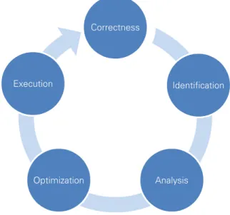
Figure 2.1: Optimization cycle: starting with correctness checking, identifying inefficient program phases, analyzing these program phases, optimizing the application, and execution.

(14)

The optimization process for parallel applications consists of five basic steps that are shown in Figure 2.1. The first step is debugging and correctness checking to ensure a correct program execution. The second step is to get a coarse view on the application behavior and identify program phases that contain irregular or inefficient behavior. These program phases can then be reviewed and analyzed in detail. The gained information can be used to optimize either the algorithm itself or its adaption to the current hardware and software stack and, finally, execute the revised application.

Within this optimization cycle, performance analysis covers the identification and analysis steps and provides input for optimization. Appropriate performance analysis tools assist developers not only in identifying performance inefficiencies but also in understanding the behavior of their applications on the complex and heterogeneous HPC systems. Furthermore, they help to analyze the performance inefficien-cies and provide insight into the exact course of events during the application runtime.

The variety of concepts and according tools can be categorized by their approach for capturing, recording, and presentation of performance information [Jai91], as shown in Figure 2.2. Within the first stage, data capturing, there are two different methods. Samplingapproaches interrupt a running application at arbitrary points (usually fixed intervals) and record the current state of execution. Whereasevent-based

methods record the state changes in the program execution, so called events, e.g., entering or leaving a code region. While the accuracy of sampling approaches relies on their frequency, event-based methods record every predefined runtime event, which means, the accuracy can be defined a priori. Vice-versa, sampling approaches can regulate the introduced measurement overhead and the memory allocation with their sampling frequency, while the overhead and memory allocation of event-based methods correlates with the frequency of the predefined runtime events.

Data Presentation Data Recording

Data Capturing Sampling Runtime Events

Tracing Aggregation Timelines Automatic Analysis Results Profiles

Figure 2.2: The three stages of performance analysis: data capturing, data recording, and data presenta-tion. Arrows indicate possible transitions between the stages.

The generated data from both approaches can then be eitheraggregated to summaries about different performance metrics or stored individually by keeping the precise time stamp and further specific metrics for each sample or event, called tracing. Aggregation approaches (also called profiling approaches1₎

immediately combine the data of new samples or events with previously recorded data. With its nature of summarization this method decreases the amount of data that needs to be stored during runtime. In contrast, tracing records each sample or event individually. It keeps every recorded state (sample) or state change (event) intact, which allows an exact reconstruction of the program behavior – with an accuracy

1_{Since aggregated data from samples or events can only be presented in the form of profiles, the method of aggregating data}

(15)

2.1. PERFORMANCE ANALYSIS 7

based on either the sampling frequency or the predefined events. Consequently, tracing data includes aggregated data because aggregated summaries always can be computed from a trace.

The aggregated and traced data can be presented in three different ways: profiles, timelines, and au-tomatically generated analysis results. Profiles display a summarization of one or more performance metrics over the entire program runtime or separately for defined program phases. These summaries can be represented as plain text, tables or charts. A typical example is the distribution of the overall program runtime over the different code regions or the total number of invocations for each code region. Profiles can be derived directly from aggregated data or computed from traces. Timelines display the initially recorded program states or state changes along a time axis and, therefore, show the exact state of the application at any give time. Since this approach requires the exact states or state changes it can only be derived from tracing data. Next to profiles and timelines that represent the recorded data, there are approaches that evaluate the recorded data and enrich the presentation of either profiles or timelines with results of an automatic analysis. Automatic analyses usually focus on the detection of typical inefficient patterns or the evaluation of specific performance metrics that might hint inefficient behavior.

While there are multiple possible combinations within these three stages, there are two well-established paths:profiling, which usually refers to aggregated events presented as profiles, andevent tracing, which visualizes event traces in the form of timelines or leads to an automatic analysis. Both approaches differ greatly in memory allocation and extractable information. Due to the summarization, the memory allo-cation for profiling correlates only with the number of different performance metrics that are recorded, whereas, the memory allocation of event tracing correlates with the number of runtime events. While single events are rather small, event tracing frequently results in huge data volumes. In fact, the large amount of collected data, in particular, for massively parallel or long running applications is one of the most urgent challenges for event-based monitoring tools.

Despite this drawback, event tracing is an essential technique since the exact communication behavior and many performance inefficiencies can only be identified with event tracing. Two prominent per-formance issues are excessive wait time in communication operations and load imbalances [Boe14]. Excessive wait time in communication, so called wait states, are usually caused by two communication partners that enter a communication operation not properly synchronized, i.e., either the sender or re-ceiver enters to late. While profiling can only hint inefficient communication behavior in general based on the total time spent in communication operations, event tracing can uncover each individual ineffi-cient communication operation and its cause [Boe14]. The conglomeration of these wait states reveals the critical path in the execution of an application, as well. Load imbalances can occur in different forms. Figure 2.3 shows an example that helps to distinguish between the analysis capabilities of event tracing and profiling for load imbalances. The left side depicts a timeline visualization of a load imbalance with four synchronizations depicted by the vertical grey lines. On the right side, a profile visualization shows the aggregated runtime for each process. The upper part represents a static load imbalance, i.e., the process that takes longer for the execution (red) is the same in each program phase. In contrast, the bottom part represents a dynamic load imbalance where the processes that causes the delay is different in each program phase. The timeline based on event tracing reveals both imbalance patterns, while the profile based on aggregated data only reveals the static imbalance, i.e., in this case it is impossible to detect the dynamic load imbalance. In addition, event tracing enables the detection of the critical path in both cases, which is in this example the sequence of the red program phases in the timeline.

(16)

Pr oc es se s Time Pr oc es se s Time Processes A gg re ga te d ru nt im e Processes A gg re ga te d ru nt im e

Figure 2.3: Analysis capabilities of tracing vs. profiling: static (top) and dynamic (bottom) load imbal-ance presented as timelines (left) and profiles (right).

Research in performance analysis also hints towards a trend that the gap between both approaches is shrinking. Profiling approaches, on the one hand, use techniques such as phase-based profiling [MSM05, CBL07] or call-path/call-graph profiling [GKM82, SWW09] to gain more information than with flat profiles over the entire runtime. On the other hand, event tracing approaches try to either reduce the number of predefined runtime events, e.g., only record the communication behavior, or try to reduce the number of stored events to cope with the tremendous data volumes.

2.2 Performance Analysis Tools Overview

After an introduction to the field of performance analysis, this section provides on overview about es-tablished performance analysis tools and their approaches. Figure 2.4 shows a classification of these performance analysis tools. Since, data aggregation usually leads to a profile presentation and tracing data is usually visualized with timelines, the figure uses the terms profiling and tracing for an easier-to-read presentation. While there are many more academic and commercial tools that focus on single aspects of performance (e.g., only communication [VM01, NRM+09]), this classification includes tools that use a general approach and analyze multiple performance relevant metrics.

Event-based Profiling Tools

Profiling tools based on events, also called instrumentation profiling tools, are gprof [GKM82], IPM [FWS10], and Periscope [BPG10].

In this list,gprof is one of the oldest and probably most used tools, since it is included in many Unix systems. It supports event-based call-graph profiling but also profiling based on sampling. Gprof results in a basic text output that shows typical profile information such as time spent in code regions or their number of invocations.

The Integrated Performance Monitoring (IPM)is a collaborative project between the National Energy

(17)

2.2. PERFORMANCE ANALYSIS TOOLS OVERVIEW 9 GProf IPM Periscope perf tools pprof Allinea MAP Vampir Scalasca TAU Paraver Score-P Paradyn HPC Toolkit Intel Vtune Profiling Tracing Event-based Sampling

Figure 2.4: Classification of performance analysis tools.

Diego Supercomputer Center (SDSC). It focusses primarily on communication, computation, and I/O and provides an output in the form of tables, charts and plots.

Periscopeis an automatic performance analysis tool developed at Technische Universität München,

Ger-many. It consists of a front-end integrated in the Eclipse IDE2 and a hierarchy of communication and analysis agents. Each of the analysis agents searches autonomously for defined patterns that indicate inefficient behavior in a subset of the application processes. The results are fed back to the Eclipse IDE and relate to the according source code parts.

Statistical Profiling Tools

Profiling tools that aggregate sampling data, also called statistical profiliers, are the Linux perf tools [Wea14], pprof [GG14], Allinea Map [All14] and the aforementioned gprof [GKM82].

TheLinux perf tools(previosly Performance Counters for Linux (PCL)) is part of the linux kernel since

version 2.6.31, which allows statistical profiling of the entire system, both, kernel and user space code.

TheGoogle performance toolsinclude a profiling tool based on sampling. With the also contained pprof

tool the gathered data can be translated to a plain text output or a graphic call graph annotated with timing information [Ghe08].

Allinea’s MAPtool presents itself as the most elaborated of the statistical profilers. It implements

adap-tive sampling rates and provides a sophisticated graphical user interface. However, the tool is proprietary and its approach is not scientifically evaluated.

2

(18)

Sampling-based Tracing Tools

Tracing tools based on samples are the HPCToolkit [ABF+10] and Intel’s VTune [Rei05]. Furthermore, there are event-based tracing tools that support sampling, too, e.g., Paraver and Score-P (see below).

TheHPCToolkit, developed at Rice University, is a sampling-based tracing tool that supports three

dif-ferent visualization methods: code-centric (i.e., a call-path profile), thread-centric, and time-centric (i.e., a timeline) [MCA+14]. A unique feature of HPCToolkit is its ability to combine the recovered static program structure with dynamic calling context information to attribute performance metrics to calling contexts, procedures, loops, and inlined instances of procedures [TMCF09].

Intel’s VTune in its current version as Intel VTune Amplifier 2015 [Int14a] is a proprietary tool that

provides basic profiles and timelines.

Event-based Tracing Tools

The fourth category, event-based tracing tools, contains analysis tools such as Vampir [NAW+96], the Scalasca toolset [GWW+10], the Tuning and Analysis Utilities (TAU) [SM06], the Paraver toolset [SLGL10], and the Paradyn toolset [MCC+95]. Furthermore, there is the measurement infrastructure Score-P [KRM+12], which serves as a unified monitoring system for the analysis tools Vampir, Scalasca, and Tau. Because they are the primary target of the contributions presented in this thesis, these tools are covered in more detail in the next section.

2.3 Event-based Trace Analysis Tools

This section narrows down the focus on well-established event-based performance analysis tools and their general approaches. While there are many more academic and proprietary approaches [MCLD01], for instance, Paradyn [MCC+95], the Intel Trace Analyzer [Int14b], OpenSpeedShop [SGM+08], and Jumpshot [ZLGS99], this section focuses on tools that represent a distinguished class of features. Be-cause other tools share similar approaches, they are not covered separately. Furthermore, this section provides a basis for the discussion of the current challenges in event-based tracing presented in the next section and allows to assess requirements for enhancements to the current approaches.

2.3.1 The Vampir Toolset

Vampir (Visualization and Analysis of MPI Resources) [KBD+08] is a well-proven and widely used toolset for event-based performance analysis in the high performance computing community. It consists of the Vampir trace visualizer [NAW+96, BN03, BWNH01] and the VampirTrace measurement envi-ronment [MKJ+07, ZIH14]. The Vampir visualizer is available as a commercial product since 1996. Its development started at the Center for Applied Mathematics of the Research Center Jülich, Germany and is continued at the Center for Information Services and High Performance Computing (ZIH) of the Technische Universität Dresden, Germany. Its counterpart, the VampirTrace measurement environment is available as open source software since 2006. It supports all major parallel paradigms and accelerator APIs simultaneously, e.g., message passing (MPI), threading (OpenMP, Pthreads), and accelerator APIs (CUDA, OpenCL). Within the collaborative project SILC [SILC09] the unified measurement infrastruc-ture Score-P was developed, which is replacing VampirTrace now (see Section 2.3.5).

(19)

2.3. EVENT-BASED TRACE ANALYSIS TOOLS 11

Today, the Vampir trace visualizer includes a scalable, distributed analysis architecture called Vam-pirServer [BNM03, BMSB03]. The VamVam-pirServer architecture enables the scalable processing of both, large amounts of trace data and large numbers of processing elements. This architecture consists of a visualization client, a master process, and a number of distributed workers (see Figure 2.5). The client is intended to run on a user’s local system and visualizes the display information received from the server. The master process of the server handles the requests from the client and distributes partial requests to the workers. The workers evaluate disjoint parts of the trace data, usually a subset of locations of the monitored application, and send the results to the master. The master communicates these results in the form of already composed display information to the client, hence, it requires only a moderate network connection between client and server. Small, local traces can also be evaluate directly by the client.

Dresden, September 15th Comprehensive Performance Tracking with Vampir 7.0

Slide 4

01 New Performance Browser

Vampir Components Vampir Trace Vampir Trace Trace File (OTF) Vampir 7.0 Trace Bundle VampirServer CPU CPU CPU CPU CPU CPU CPU CPU Multi-Core Program

CPU CPU CPU CPU

CPU CPU CPU CPU CPU CPU CPU CPU

CPU CPU CPU CPU

CPU CPU CPU CPU CPU CPU CPU CPU

CPU CPU CPU CPU

Many-Core Program

Figure 2.5: Vampir/VampirTrace architecture overview. VampirTrace (left) records events from the par-allel application. The resulting trace file is processed either directly by the Vampir client or by the VampirServer in the case of large parallel programs (taken from [BHJH10]).

As stated before, event-based tracing tools present the tracing data in the form of timelines along with summarized profile information and automatically derived analysis results. The main visualization ap-proaches of Vampir, exemplary for many similar tools, are detailed below.

Master Timeline Display

A master timeline visualization generates a visual representation of the application behavior over time in the form of a space-time diagram. It represents the active code region over time for each location on the horizontal axis and the selected locations on the vertical axis. Whereas each code region or group of code regions is marked as a segment of a location bar with a specific color for the time it is active. Communication and interaction between locations are represented by arrows and lines. For each element of the master timeline detailed context information is available, when selected.

While the initial representation of the timeline displays the activity of all locations along the entire application runtime, zooming is the method to gain more detailed information. Zooming and scrolling can be executed in the horizontal and vertical dimension to change the shown time interval or subset of locations, respectively. Figure 2.6 shows an example of a global timeline zoomed to a time interval of 0.5 seconds. It is based on a trace of the Weather Research and Forecast Model (WRF) [MDG+04].

(20)

Process Timeline Display

Process timelines are similar to global timelines but focus on a single location. The vertical dimension is used to visualize the hierarchy and call dependencies of the code regions by arranging the segments according to their calling depth (see Figure 2.7). Horizontal and vertical zooming and scrolling can be applied in the same way as for global timelines. The process timelines can also be aided by available performance metrics shown as graphs over time. For a detailed comparison of a subset of processing elements multiple process timelines can by displayed simultaneously with aligned time intervals.

Summary Charts

The summary chart displays statistical information about code regions or groups of code regions such as total or average inclusive or exclusive runtime or number of invocations. This information can be gathered from a single location or groups of such and can be shown as pie charts or histograms (see Figure 2.8). While this information is very similar to profiles, the summary charts can be computed for arbitrary time intervals usually selected via a timeline display. Furthermore, all per processing element summaries can be displayed side by side to compare the general behavior of the individual processing elements.

Communication Matrix

The communication matrix shows information to analyze the communication behavior of a measured application such as number of messages, volume, transfer time, and data rates as minimum, average, and maximum values. The values are displayed as two-dimensional matrix with color-coded entries (see Figure 2.9), which allows an easy identification of communication patterns.

Display Arrangement, Performance Radar, and Trace Comparison

All of the above mentioned displays and some more, e.g., for call trees, performance metrics, and location clustering, can be arranged freely within one application window. Figure 2.10 shows an example based on WRF with a clustered process summary chart (i.e., classes of locations with similar behavior are represented only once), a global timeline, and a performance metric display showing the floating point operations per second on the left side, and the function summary, function legend, and call tree on the right side. All these displays are synchronized, thus, whenever the time interval is change within the global timeline, all other displays are re-computed accordingly.

Next to a location local presentation of a performance metric, a color-coded presentation including all locations allows a direct comparison of differences in the behavior of the processing elements regarding a specific performance metric – the so called performance radar. Figure 2.11 shows the floating point op-erations per second for all locations, which allows in this case an easy identification of compute intensive application phases.

Furthermore, the custom display placement also supports a comparison of multiple traces, which, for instance, is useful for comparing application runs with different parameters or the evolvement of an application in different optimization stages. In addition, approaches for a structural comparison of traces can be applied [WBB12, WMS+13].

(21)

Figure 2.6: Vampir master timeline display showing 16 MPI processes of a WRF measurement zoomed to a time interval of 0.5 seconds (taken from [GWT14]).

Figure 2.7: Vampir process timeline display showing the call hierarchy of the code regions for process 0 from the example in Figure 2.6 (taken from [GWT14]).

(22)

Figure 2.8: Vampir summary chart showing the accumulated exclusive runtime for different function groups as pie chart and histogram (taken from [GWT14]).

(23)

Figure 2.10: Vampir custom display arrangement including a clustered process summary chart, a global timeline, and a performance metric display on the left side, and a function summary, func-tion legend, and call tree on the right side. (taken from [GWT14]).

Figure 2.11: Vampir performance radar showing the floating point operations per second, which allows an easy identification of compute intensive phases (taken from [GWT14]).

(24)

2.3.2 The Paraver Toolset

The Paraver tool set consists of the Paraver visual performance analyzer [CEP01b] and the Extrae mea-surement environment [BSC14]. In addition, the Dimemas tool [CEP14] allows trace-based replay to simulate program behavior of a recorded application under alternative conditions such as different CPU speed or different network characteristics. All three tools are developed at the Computer Science devision at the Barcelona Supercomputing Center, Spain since 1991 (partly under different names).

The Extrae monitor supports the recording of all major parallel and accelerator paradigms simultaneously much like VampirTrace. As a unique feature, Extrae records events generated by code instrumentation and sampling probes together. This approach provides additional information between runtime events, which can be useful for long or un-instrumented code regions [BSC14].

The Paraver toolset uses its own trace format, which supports only three basic event record types: states that associate a value for a stream during a time interval, events that represent a punctual event on a stream, and relations that relate two events on two different streams together [CEP01a]. The rather abstract description of these record types originates in their so called semantic free design. Thus, all specific events are mapped to one of these basic record types, e.g., code region enter/leave to states, performance metrics to events, or a point-to-point communications to relations.

The Paraver trace visualizer uses a semantic module to generate a semantic value (numeric value) for each object to be represented, which is a function of time that is computed from the records that correspond to the object. These objects belong to either of two fixed hierarchies: programming model (workload, application, task and thread) and resources (system, node and CPU) [CEP01a]. For both, the semantic value is hierarchically computed according to the general object model structure. Paraver uses three presentation modules: visualization (timelines), textual and statistics (profiles). Each of them handles one of the three types of records [BSC10]. Figures 2.12 – 2.14 show examples of these three presentations.

(25)

Figure 2.13: Paraver’s textual view opens when clicking on a timeline (taken from [BSC10]).

Figure 2.14: Paraver statistics view showing a tabular view of time spent in MPI functions and a com-munication matrix (taken from [BSC10]).

(26)

2.3.3 The Scalasca Toolset

The Scalasca toolset represents a different performance analysis approach than the aforementioned tools. Unlike the performance visualization tools, it applies an automatic analysis to identify patterns of ineffi-cient application behavior. The resulting performance report is presented in a hierarchical viewer called CUBE. Scalasca is developed at the Forschungszentrum Jülich, Germany and the German Research School for Simulation Sciences, Germany. Its predecessor Kojak [WM03] was additionally developed at University of Tennessee in Knoxville, USA. While previous versions included a trace monitor, today, Scalasca uses the unified measurement environment Score-P for trace generation.

The parallel trace analyzer Scout [SDT14a] performs the automatic analysis in Scalasca by searching for predefined patterns of inefficient application behavior. Each identified pattern is given a severity rating ranging from noncritical to critical to allow an easy identification of the most severe performance issues. All predefined patterns are categorized in a hierarchy from general to specific. Typical patterns of ineffi-cient behavior include idle threads or wait times in global or point-to-point communication. Figure 2.15 shows two prominent examples of wait times in point-to-point communication due to unsynchronized messages: the so-called late sender and late receiver pattern. The severity of both patterns is derived from the delay between matching calls, i.e., the longer a communication partner waits the higher the severity. A complete list of performance properties can be found in [SDT14c].

Pr oc es se s Time Time Time Send Receive Send Send Receive Receive Wait Wait Pr oc es se s Pr oc es se s

Figure 2.15: Patterns for point-to-point communication: synchronized (left), late sender (center), and late receiver (right), which cause wait times for the sender and receiver, respectively.

The results of the automatic analysis are stored in a single XML file, which is the input for the CUBE display [GSS+12]. It displays the information in three dimensions side by side: a metric dimension, a program dimension, and a system dimension (see Figure 2.16). The metric dimension contains a set of metrics, such as communication time or cache misses that represent the patterns found by Scout. The program dimension shows an application call tree, which includes all call paths onto which metric values can be mapped. The system dimension represents the parallel locations, which can be processes or threads depending on the parallel programming model [SDT14b]. Alternatively, the system dimension can display the performance properties within the system topology (see Figure 2.17).

Each dimension is organized in a hierarchy in the form of weighted trees where the severity rating of each tree node is the aggregation of its sub-trees when collapsed and contains only its own severity when expanded. The severity values are represented by numeric values (absolute or relative), as well as a color-coding, which supports a quick visual perception of the most severe performance properties. Furthermore, the three displayed dimensions are synchronized, so that selecting a sub-tree restricts the other displays to the selected metric. Since the Scalasca approach automatically detects predefined per-formance inefficiencies, it allows a convenient and low-key identification of typical perper-formance issues.

(27)

Figure 2.16: Cube display with its three dimensions: metric tree, call tree, and system tree with color-coded severities (taken from [SDT14b]).

Figure 2.17: Cube display showing the performance metrics mapped to the three-dimensional system topology (taken from [GWW+10]).

(28)

2.3.4 The Tuning and Analysis Utilities (TAU)

The Tuning and Analysis Utilities (TAU) provide tools for event-based and sample-based tracing, profil-ing and profile analysis. For the analysis of event-based traces TAU relies on the aforementioned tools: "We made an early decision in the TAU system to leverage existing trace analysis and visualization tools. However, TAU implements it own trace measurement facility and produces trace files in TAU’s own format." [SM06]. Consequently, TAU includes trace file converters to translate TAU traces into formats used by theses tools. However, for large trace files such a conversion might imply a huge effort. Hence, TAU also suggests using Score-P for tracing to generate OTF2 traces [TAU12b] (see Section 2.3.5). The TAU tracing tools provide two distinct approaches to enhance functionality. The first is PDT [LCM+00], that allows selective source code instrumentation. The second includes early approaches for online performance analysis, one using parallel profiling analysis over MRNet [NMM+08] and the other using file-based online trace analysis with VampirServer [BMSB03]. Furthermore, TAU supports many advanced profiling features such as phase-based and call-graph profiling and its own visualization tool ParaProf. Figures 2.18 and 2.19 show two example visualizations.

Figure 2.18: ParaProf showing aggregated exclusive runtime per location of each code region. The un-stacked bars view (right) allows a comparison of individual code region across location (taken from [TAU12a]).

Figure 2.19: ParaProf 3D visualization allows to show two metrics (by height and color) for all code regions and locations (taken from [TAU12a]).

(29)

2.3.5 Score-P and the Open Trace Format 2

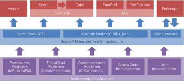
The previous sections focussed on the analysis functionality of the different tools, which equals the third stage of performance analysis: data representation. Each tool workflow includes its own measurement tool that covers the first and second stage: data capturing and data recording. However, the differ-ent measuremdiffer-ent environmdiffer-ents VampirTrace (Vampir), Extrae (Paraver), Scalasca, and TauTrace (TAU) share very similar techniques for event generation and recording. This led to the idea of joint devel-opment and evolution of a unified measurement infrastructure. Today, Score-P [KRM+12] is the joint measurement infrastructure for the analysis tools Vampir, Scalasca, Periscope, and TAU. It comprises the measurement functionality of these tools into a single infrastructure, which provides a maximum of con-venience for users next to a reduction of redundant effort in tool development. The Score-P measurement infrastructure allows profiling, event tracing, and online analysis. It contains the code instrumentation functionality supporting various methods and performs the runtime data collection. Figure 2.20 shows an overview of the Score-P architecture and its interfaces to the supported analysis tools.

Instrumentation Wrapper

Vampir Scout Cube ParaProf PerfExplorer Periscope

Event Traces (OTF2) Call-path Profiles (CUBE4, TAU) Online Interface

Process-level Parallelism (MPI, SHMEM) Thread-level Parallelism (OpenMP, Pthreads) Accelerator-based Parallelism (CUDA, OpenCL) Source Code

Instrumentation InstrumentationUser

Scalasca TAU

Score-P Measurement Infrastructure

Figure 2.20: Architecture of the Score-P instrumentation and measurement infrastructure and its inter-faces to supported analysis tools.

Score-P captures all major paradigms through the following instrumentation techniques:

• Code regions via compiler instrumentation,

• MPI and SHMEM via library interposition,

• OpenMP source code instrumentation using Opari2 [LDTW14],

• Pthread instrumentation via GNU ld library wrapping,

• CUDA, OpenCL instrumentation,

• Selective source code instrumentation via the TAU instrumenter (PDT) [LCM+00],

• Binary instrumentation using Cobi [MLW11], and

• Manual user instrumentation.

While the online interface provides direct access via TCP/IP for online analysis tools such as Periscope, the interface for the other analysis tools is realized by various file formats. For the profiling tools Cube, ParaProf, and PerfExplorer Score-P uses their native formats Cube [SDT14b] and TAU [TAU12a]. Event tracing data is stored within an OTF2 archive, which is covered next.

(30)

The Open Trace Format 2 (OTF2)

Event trace data formats of the different tools have many similarities just like the measurement tools themselves [Knu08, EWG+12]. The similarities are also shown in the existence of various converters between most formats [SM06]. Consequently, a unified event trace data format has been developed along with the unified measurement infrastructure. The Open Trace Format 2 (OTF2) [EWG+12] is a highly scalable, memory efficient event trace data format and support library. It is the new standard trace format for Vampir, Scalasca, and TAU. OTF2 is the common successor for the Open Trace Format (OTF) [KBB+06] used by Vampir/VampirTrace and the Epilog trace format [WM04] used by the Scalasca toolset. It preserves the essential features and record types of both and introduces new features such as support for multiple read/write substrates, in-place time stamp manipulation, and on-the-fly token translation. In particular, it avoids copying during unification of parallel event streams.

Since the Open Trace Format 2 is the starting point for the contributions of this thesis, this section presents it in detail as an example similar to many other event trace formats such as the Paraver Trace Format [CEP01a], the TAU trace format [SM06], the Structured Trace Format of the Intel Trace Analyzer [Int14b], as well as its two predecessors OTF and Epilog. In addition, OTF2’s integration in multiple analysis tools allows a broad application of the contributions of this thesis (see Section 6).

The Open Trace Format 2 stores all runtime events in the form of trace records, which can be categorized in event records and definition records.

Event Records

Event records mark runtime events and consist of three parts: first a record token that defines the type of an event, second an exact time stamp telling when the runtime event occurred, and third, event spe-cific attributes. They contain all information to entirely reconstruct or replay the application execution behavior. The most common event records are [OTF14]:

• Entering and leaving a code region with an identifier of the code region,

• Sending and receiving an MPI messages storing sender, receiver, communicator, tag, and size,

• Collective MPI operations with the type of collective operation and the communicator,

• Begin and end of OpenMP parallel regions,

• Fork and join of thread teams, and

• Hardware performance metrics with type and value.

Definition Records

Within the event records all references are defined in the form of identifiers, e.g., for the code region in an enter/leave record, or sender and receiver in point-to-point messages. This allows a much higher memory efficiency in comparison to storing names, labels, and descriptions within each event record, in particular, since many of these are referenced repeatedly. The translation of these identifiers is stored within the definition records. The most common definition records are [OTF14]:

• Code regions containing their name, description, and source code location,

• MPI Communicators with their name and communication partners, and

(31)

Furthermore, there are definition records that describe the global properties of a measurement like:

• System layout, e.g., a system tree,

• Locations that describe the recorded processing elements,

• The resolution of used time stamps, and

• Various types of groups, e.g., for locations and code regions.

A complete list and a detailed description of all event and definition records can be found in [OTF14].

Read and Write Interface

The Open Trace Format 2 includes a support library that provides interfaces for read and write access to the trace data. The standard access to the trace data is in temporal order, i.e., all events must be written with monotonic increasing time stamps. When reading the trace data, the event information is delivered in the form of user-defined call back handlers in the same temporal order.

All events are separated in event streams that represent exactly one location, which results in one event file per location when the data is stored on the file system. This renders the information on which location an event occurred unnecessary within each single event stream and allows a more efficient storage than mixed-stream formats such as its predecessor OTF. Furthermore, this approach supports an efficient parallel reading of the individual event streams.

Next to the event files for each location, there is a local definition file for each event location that contains mapping tables to convert local identifiers into identifiers within a global scope. Furthermore, there is a global definition file that describes all identifiers within the global scope, i.e., the entire measurement, and the so called anchor file, which serves as an entry point for the OTF2 archive. Figure 2.21 shows the basic file layout of an OTF2 archive.

Anchor File

<ArchiveName>.otf2 Global Definition File<ArchiveName>.def

Event Files

<ArchiveName>/<#>.evt

Local Definition Files

<ArchiveName>/<#>.def

Figure 2.21: Layout of an OTF2 archive containing an anchor file as entry point, one global and multiple local definition files, and event files with records of runtime events.

(32)

2.4 Challenges in Event-based Tracing and Related Work

While the previous sections present a general overview on event-based performance analysis, this section focuses on methods related to the concepts of this thesis. This section introduces three urgent challenges in the field of event-based performance analysis and current approaches coping with these challenges. These challenges are, first, scalability in the number of processing elements, second, the management of the enormous data volumes, and, third, the reduction of measurement bias.

2.4.1 Scalability

To help users in the development of scalable software, performance analysis tools themselves must be scalable to the same extend – or even one step ahead. Current HPC systems ranging up to 3 million processing elements [Top14] require software and workflows with extreme levels of concurrency. Mon-itoring applications at this scale and beyond results in tremendous amounts of event tracing data spread across millions of files; one file for each recorded location. While high-end parallel file systems for such machines are usually equipped to provide enough disk space and sufficient I/O bandwidth, the creation of millions of parallel files is entirely infeasible with all existing parallel file systems [ISC+12]. Request-ing more than a few thousand file creations per second affects all jobs and users on a machine. Exact numbers vary on different machines and parallel file systems from 4,000 [ISC+12] to 10,000 [AEH+11] maximum file creations per second.

The reason for this limitation is the handling of file system meta data. Common HPC parallel file sys-tems such as GPFS [SH02] and Lustre [Sun08] focus on increasing data bandwidth, which is primarily achieved by adding more disk drives and more disk controllers. However, large amounts of hardware cannot improve meta data performance since the limiting factors are the number of simultaneous oper-ations and their latency. For massively parallel I/O requests, in particular file creation, their latency has the potential to become the major bottleneck [AEH+11]. In fact, for event tracing tools this meta data wall is one of the most challenging limitations already occurring for systems with tens or hundreds of thousands of cores – not even thinking about systems with several millions of cores arising within the next years [BBC+08].

Two approaches that are dealing with the file system limitations and have been applied to event tracing are SIONlib [FWP09] and the I/O Forwarding Scalability Layer (IOFSL) [ISC+12]. Both approaches merge many logical files into a single or a few physical files. While SIONlib relies on the file system’s capability to handle large sparse files to pre-allocate segments for the logical file handles within a single file, the I/O Forwarding and Scalability layer, as the name suggests, provides an I/O forwarding layer to offload I/O requests to dedicated I/O servers that can aggregate and merge requests before passing them to the actual file system.

The IOFSL approach was applied to a full Cray XT5 system measurement with 200,448 cores using the VampirTrace measurement environment [ISC+12]. SIONlib was used in combination with Scalasca to measure 294,912 cores on a BlueGene/P and the aforementioned system [WGM+10].

However, both approaches are currently limited to a subset of systems and in their general applicability. The IOFSL approach requires resources hosting the I/O forwarding servers, which would be best placed on a system’s dedicated I/O nodes. But user access to these nodes is usually restricted or impossible. Thus, the I/O forwarding servers can only be deployed on compute nodes reducing the total compute

(33)

2.4. CHALLENGES IN EVENT-BASED TRACING AND RELATED WORK 25

capability and limiting network and I/O bandwidth. In addition, starting additional server nodes with the application must be supported by the corresponding batch system. SIONlib, on the other hand, requires no server processes but causes unforeseeable synchronization in the parallel application execution, which is critical for event tracing. Furthermore, it depends on MPI for internal coordination, which is infeasible for monitoring non-MPI parallel applications.

Both approaches still cause noticeable overheads for file interaction and have only been demonstrated for small benchmarks with minimal data volumes [ISC+12, WGM+10]. The file interaction overhead in the aforementioned studies was reported with 71 seconds for IOFSL and ten minutes for SIONlib on the BlueGene/P system, which is still very high compared to the small data volumes written. Nevertheless, both approaches achieved a remarkable decrease compared to direct POSIX I/O with a factor of about three for IOFSL and a decrease from 89 to ten minutes for SIONlib.

Both studies demonstrated a drastic improvement over direct file interaction, which pushed the barrier an order of magnitude higher with justifiable overhead. Considering the overhead, the small demonstrated benchmarks, and the aforementioned restrictions, the limitations of event tracing imposed by parallel file systems are still not overcome and remain an unmet challenge.

2.4.2 Data Volumes

As stated before, event tracing can produce enormous amounts of data that need to be handled efficiently. Moreover, trace analysis tools must provide methods to support the user in getting useful information out of this overwhelming amount of data.

Data Volumes in Trace Recording

While the size of a single event record is typically only a few bytes, high event frequencies rapidly generate tremendously huge data volumes. The reviewed applications and application kernels in this thesis (see Section 5.1) show event rates of 50,000 to two million events per seconds per location, which is underlined by other studies [ISC+12]. Given an average event size of 10 bytes this would result in about 0.5 to 20 MiB per second and 300 MiB to 12 GiB for a measurement of 10 minutes. For long-running applications, such as the reviewed Gromacs package [HKS08], a full production run can produce up to 12 TiB per location (see Section 5.4). Of course, this data volumes must be multiplied with the number of recorded locations, which leads to even higher data volumes for large-scale applications. While these data volumes require extraordinary amounts of disk space, for event-based trace recording the data volumes per location are of primary importance since main memory and I/O bandwidth are usually proportional to an increase in core counts.

General Purpose Compression

To cope with large data volumes most tracing approaches use general purpose compression libraries such as the well-establish zlib [DG96] based on the the Lempel-Ziv 77 compression algorithm [ZL77] that provides a good trade-off between compression ratio and overhead [SL11]. While LZ77 compression, as most compression algorithms, depends on the input data, event trace data is typically compressed by a factor of about three to four [WKN12]. Due to the introduced overhead, general purpose compression is not applied on data within the memory buffer but when storing data to the file system.

(34)

Encoding Optimizations

In contrast to post-mortem general purpose compression, encoding optimizations of the trace format itself provide a trace size reduction within the memory buffer and the resulting trace file. However, previous enhancements in the encoding reduce trace sizes much less than general purpose compression algorithms [EWG+12]. Still, the discrepancy in size reduction between encoding and general purpose compression hints to unexploited potential in current encoding approaches.

Statistical Clustering

Statistical clustering [NRR97] exploits similarity in parallel application behavior to group processes with similar behavior in a way that all processes within the same group or cluster are more similar to each other than to those in other groups. The data reduction is achieved by keeping only a single representative for each cluster. Consequently, the compression factor for a single cluster equals the number of members. In the case of multiple clusters the total compression depends on the number of members in each cluster and their trace size. The Extrae trace monitor [BSC14] combines statistical clustering [LGS+10] with spectral analysis based on wavelets [LCS+11] to detect iterative patterns within the application, as well.

Pattern Aggregation

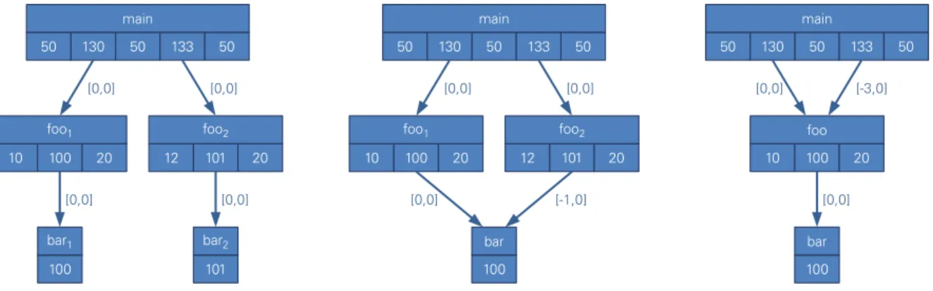
Furthermore, there are approaches that use pattern aggregation to reduce trace sizes. These approaches try to detect recurring patterns either within each event stream, e.g., iterations, or across different event streams where, especially, SPMD (single program multiple data) applications contain redundant paral-lel behavior. Compressed Complete Call Graphs (cCCG) [KN05a, KN05b, KN06] are rooted directed acyclic graphs that combine regular patterns into common sub-trees. The cCCG data structure uses the caller information and time deviations to group leave nodes, i.e., if two calls to the same function vary less than a predefined threshold, they are grouped together. In the same way are all intermediate nodes combined when their caller information matches, they have common sub-trees, and their duration devi-ates less than the given threshold. Figure 2.22 demonstrdevi-ates the compression in an Complete Call Graph for a simple example. The proposed approach also presents techniques for optimized cache utilization for the graph node and splitting methods to avoid wide graph nodes [KN06].

10 100 20 foo1 12 101 20 100 101 foo2 bar1 bar2 50 130 50 133 50 main [0,0] [0,0] [0,0] [0,0] 10 100 20 foo1 12 101 20 100 foo2 bar 50 130 50 133 50 main [0,0] [0,0] [0,0] [-1,0] 10 100 20 foo 100 bar 50 130 50 133 50 main [0,0] [-3,0] [0,0]

Figure 2.22: Successive compression in a CCG. The first graph (left) shows an uncompressed CCG. Since both calls to functionbarare compatible they are replaced by a reference (middle). Runtime deviations are propagated to the parent node as a deviation interval [-1, 0]. As both calls tofooreference the same child node they are grouped together, as well (right) [KN06].

(35)

2.4. CHALLENGES IN EVENT-BASED TRACING AND RELATED WORK 27

In addition, a study by Mohror and Karavanic [MK09] evaluates different pattern-based methods for trace compression against several criteria including size reduction and introduced error. The ScalaTrace monitor [NRM+09] presents another pattern-based method explicitly for MPI traces, hence, it does not contain any events for code regions.

Filtering and Selective Instrumentation

Another way to reduce the size of the resulting trace files are manually or automatically applied event filters. A very common filter is the discarding of all function calls when a code region is entered more often than a predefined limit [MKJ+07, GWW+10, KRM+12]. This usually eliminates an overcharge of highly frequent calls to tiny functions, such as helper functions and get/set class methods. Optionally, filters for those functions can be determined beforehand either by statistical source code analysis or a profile run of an application [MLW11]. Selective instrumentation allows to exclude specific functions from being instrumented at all [LCM+00, MLW11]. Furthermore, it is possible to manually define which code regions are instrumented [MKJ+07, KRM+12]. The Paradyn monitor additionally allows to dynamically instrument functions during runtime [BM11] based on their approach for direct binary instrumentation [HMC94].

Data Volumes in Trace Analysis

Event-based trace analysis faces similar challenges with the growing data volumes. Since most tools ap-ply scalable analysis techniques and use either the same amount of resources for analysis as the measured application or an adequate subset [BNM03, GSS+12], the increasing data volumes caused by increas-ing core counts are a smaller challenge for data processincreas-ing than the large data volumes per location. However, the increasing data volumes with increasing core counts impose a demanding challenge for the presentation of analysis results. While automatic analysis approaches, such as an detection of root causes of wait states [BGWA10] and determination of the critical path in the application execution [BSG+12], try to pin-point to the most severe performance issues, visual analysis approaches have to circumvent limitations in the screen resolutions as well as in the human perception of information.

The limitations in screen resolution, i.e., presenting more processing elements in a timeline visualization than there are pixels, are passed with an intelligent selection algorithm [NAW+96] or by clustering locations in groups with similar behavior [Bru08, LGS+10]. These approaches allow a reduction of information presented to the user on a complete application representation but when the focus is reduced to parts of the application the detail is kept.

The large data volumes per location are challenging in the data processing as well as the data represen-tation. Since most analysis tools process the recorded events within their own data structures, a trace size reduction achieved by any sort of compression does not reduce the amount of data that needs to be processed and kept in the analysis data structures. On the contrary, the overhead for reading the data is increased by applying an according decompression, except for those approaches that provide options for optimized access to the compressed data structures such as cCCGs [KN06]. Only approaches that reduce trace size by reducing the number of events per location with filters or selective instrumentation allow a reduced effort in trace analysis.