Modelling Orebody Structures: Block Merging Algorithms and Block Model Spatial Restructuring Strategies Given Mesh Surfaces of Geological Boundaries

(1)

JOURNAL OFSPATIALINFORMATIONSCIENCE

Article submitted for review

Modelling Orebody Structures: Block

Merging Algorithms and Block

Model Spatial Restructuring

Strategies Given Mesh Surfaces of

Geological Boundaries

Raymond Leung

Australian Centre for Field Robotics, The University of Sydney, Australia

Received: October 13, 2019; revised: –; accepted: –; published: .

Abstract:This paper describes a framework for capturing geological structures in a 3D block model and improving its spatial fidelity, including the correction of stratigraphic boundaries, given new mesh surfaces. Using surfaces that represent geological bound-aries, the objectives are to identify areas where refinement is needed, increase spatial resolution to minimise surface approximation error, reduce redundancy to increase the compactness of the model and identify the geological domain on a block-by-block basis. These objectives are fulfilled by four system components which perform block-surface overlap detection, spatial structure decomposition, sub-blocks consolidation and block tagging, respectively. The main contributions are a coordinate-ascent merg-ing algorithm and a flexible architecture for updatmerg-ing the spatial structure of a block model when given multiple surfaces, which emphasises the ability to selectively retain or modify previously assigned block labels. The techniques employed include block-surface intersection analysis based on the separable axis theorem and ray-tracing for establishing the location of blocks relative to surfaces. To demonstrate the robustness and applicability of the block merging technique to a wider class of problem, the core approach is extended to reduce fragmentation in a block model where surfaces are not directly involved. The results show the proposed method produces merged blocks with less extreme aspect ratios and is highly amenable to parallel processing. The

1

Please do not cite

(2)

overall framework is applicable to orebody modelling given mineralisation or strati-graphic boundaries, and 3D segmentation more generally, where there is a need to delineate geographic regions using mesh surfaces within a block model.

Keywords: Subsurface modelling, geological structures, boundary correction, domain identification, block merging algorithms, spatial restructuring, mesh surfaces

1

Introduction

In mining, 3D geological models are used in resource assessment to characterise the spatial distribution of minerals in ore deposits [12]. A block model description of the geochemical composition is often created by fusing various sources of information from drilling campaigns: these include assay analysis, geophysical logging and align-ment of stratigraphic units from geologic maps during the exploration phase. Due to the sparseness of these samples, the inherent resolution of these preliminary mod-els are typically low. As the exploitation phase commences, denser samples may be taken strategically to develop a deeper understanding about the geology of viable ore deposits. This knowledge can assist miners with planning and various decision mak-ing processes [11], for instance, to prioritise areas of excavation, to develop a minmak-ing schedule [7], to optimise the quality of an ore blend in a production plant. Of particu-lar relevance to spatial modelling is that wireframe surfaces can be generated by geo-modelling software [20] [15], or via kriging [9], probabilistic boundary estimation [3] and other inference techniques [22] to minimise the uncertainty of interpolation at lo-cations where data were previously unavailable. For instance, triangle meshes may be created by applying the marching cubes algorithm [17] to Gaussian process implicit surfaces [8]. These boundary updates provide an opportunity to refine existing block models and remove discrepancies with respect to verified boundaries. The objective is to maximise the model’s fidelity by increasing both accuracy and precision subject to some spatial resolution constraint. The desired outcomes are improved localisation, reduced quantisation errors and less fragmentation. In other words, the boundary blocks in the block model should accurately reflect the location of boundaries between geological domains; smaller blocks should be used to capture the curvature of regions near boundaries to minimise the surface approximation error; the model should pro-vide a compact representation and have a low block count.

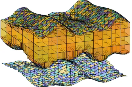
Figure 1 provides a visual summary of the primary objective. A key feature of spatial restructuring is that blocks are divided as necessary to adapt the block model to the curvature of the given surfaces. This process, known as sub-blocking, is com-monly performed in a top-down recursive manner which prioritizes splitting ahead of block consolidation. In some implementations, block consolidation is omitted alto-gether; this usually results in a highly fragmented and inefficient block representation. In this paper, surface-intersecting blocks are decomposed down to some minimum

c

by the author(s) Licensed under Creative Commons Attribution 3.0 License CC

Please do not cite

(3)

BLOCKMERGINGALGORITHMS& SPATIALRESTRUCTURINGSTRATEGIES 3

Figure 1: Essence of block model spatial restructuring given mesh surfaces

block size, then hierarchical block merging is performed in a bottom-up manner to consolidate the sub-blocks. In the ensuing sections, a framework for modifying the spatial structure of a block model using triangular mesh surfaces is first presented, the techniques underpinning each subsystem are described. Subsequently, we devote our attention to the block merging component, the algorithm is extended to support dif-ferent forms of merging constraint. The proposed methods are applicable to orebody modelling given surfaces of mineralisation or stratigraphic boundaries — see scenar-ios illustrated by [24], [10], [13], [4]; and general purpose 3D block-based modelling given other types of delineation.

2

Framework for Block Model Spatial Restructuring

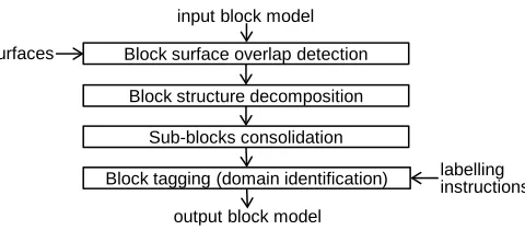
This section develops a framework for altering the spatial structure of a block model to reconcile with the shape of the supplied surfaces as depicted in Fig. 1. Without loss of generality, the input block model consists of non-overlapping blocks of varying sizes (with uniform 3D space partitioning being a special case) and the surfaces, typ-ically produced by boundary modelling techniques, represent the interface between different geological domains. The triangular mesh surfaces, together with the initial block model and block tagging instructions (class labelling directives with respect to each surface) constitute the entire input. The framework may be described in terms of four components: block surface overlap detection, block structure decomposition, sub-blocks consolidation and block tagging (domain identification) as shown in Fig. 2.

2.1 Block surface overlap detection

The goal is to identify blocks in the input model which intersect with the given sur-face(s). These represent areas where model refinement is needed in order to minimise

JOSIS, Article submitted for review

Please do not cite

(4)

4 RAYMONDLEUNG

Block surface overlap detection

Block structure decomposition

Sub-blocks consolidation

Block tagging (domain identification) surfaces

output block model

labelling instructions input block model

Figure 2: Components in the block model spatial restructuring framework

the surface approximation error. To establish a sense of scale, the input blocks (also called “parent blocks”) typically measure25×25×5m in an axis-aligned local frame, “axis-aligned” means the edges of each block are parallel to one of the (x, y or z) axes.

2.2 Block structure decomposition

Block decomposition is performed on surface-intersecting parent blocks to improve spatial localisation. This process divides each block into smaller blocks of some mini-mum size (e.g.,6.25×6.25×1.25m). These sub-blocks are disjoint and together, they span the whole parent block. Geometry tests are applied to determine which sub-block inside each surface-intersecting parent block actually intersects with a given surface. This process places blocks into one of three categories: (a) parent blocks that never in-tersect with any surface; (b) sub-blocks (inside surface-inin-tersecting parent blocks) that intersect with some surface, and (c) sub-blocks that do not intersect with any surface.

2.3 Sub-blocks consolidation

This component coalesces sub-blocks to produce larger blocks in order to prevent over-segmentation. Recall that one of the objective is to minimise the total number of blocks in the output model. Therefore, if an array of3×4×2sub-blocks could be merged into a perfect rectangular prism, it would be more efficient to represent them collectively by a single block with a new centroid and their combined dimensions.

In the event that the sub-blocks (within a surface-intersecting parent block) inter-sect with multiple different surfaces (says1ands2) then merging considerations will

be applied separately to the sub-blocks intersecting with s1 ands2. It is important to

observe that block consolidation is applied to both category “b” and category “c” sub-blocks as defined above. Also, merging of sub-sub-blocks across parent block boundaries is not permitted.

www.josis.org

Please do not cite

(5)

2.4 Block tagging (domain identification)

As a general principle, block tagging assigns abstract block labels to differentiate blocks located above and below a given surface. The objective is to support tagging with respect to multiple surfaces and two labelling policies. The first policy distin-guishes surface-intersecting blocks from non-intersecting blocks. The second policy forces a binary decision and labels surface-intersecting blocks as strictly above or be-low a surface. The scheme also offers the flexibility of using a surface to limit the scope of an update, thereby leaving previously assigned labels intact above / below a surface.

This completes our brief overview of the system.

3

Techniques

The techniques used in each component will now be further described.

3.1 Detecting block surface intersection

The method we employed for determining if an axis-aligned rectangular prism inter-sects with a triangular patch from a surface is described by Akenine-Möller in [1]. This approach applies the Separating Axis Theorem (SAT) which states that two convex polyhedra, A and B, are disjoint if they can be separated along either an axis parallel to a normal of a face of either A or B,oralong an orthogonal axis computed from the cross product of an edge from A with an edge from B. The technical details can be found in Appendix A.

In essence, block-surface intersection assessment consists of a series of “block ver-sus triangle” comparisons where the triangles considered for each block are selected based on spatial proximity. The block-triangle overlap assessment operates on one ba-sic principle: a “no intersection” decision is reached as soon as one of the tests returns

FALSE. A block-triangle intersection is found only when all 13 tests returnTRUE, when

it failed to find any separation. These tests are used to identify the surface triangles (if any) that intersect with each parent block.

To maximise computation efficiency, each block is tested against a subset of trian-gles on each mesh surface rather than the entire mesh surface. A kD-tree is constructed based on the 3D bounding boxes of each triangle. The subset includes only triangles whose bounding box overlaps with the block; only these candidates can intersect with the block. This pruning step limits the number of comparisons and speeds up compu-tation considerably. The indices harvested here can subsequently reduce the test effort in the block structure decomposition stage.

Please do not cite

(6)

6 RAYMONDLEUNG

3.2 Block structure decomposition

The key premise is to decompose surface-intersecting blocks into smaller blocks to improve spatial localisation. The basic intuition is that the surface discretisation error decreases as spatial resolution increases. Precision increases when smaller blocks are used to approximate the surface curvature where the blocks meet the surface.

Block structure decomposition entails the following. For each block (b) that in-tersects with the surface, divide it volumetrically into multiple sub-blocks using the specified minimum block dimensions (∆block_x,_min,∆_y,block_min,∆block_z,_min). The main constraints are that sub-blocks cannot overlap and they must be completely contained by the parent block whose volume is the union of all associated sub-blocks.1 Within each surface-intersecting parent block, we also identify all sub-blocks that intersect with a surface and which surface they intersect with. This is accomplished using the asso-ciative mapping [obtained during block-surface overlap detection] which limits the relevant surface triangles to a small subset for each surface-intersecting parent block. The relevant attributes captured in the output include a list of surface-intersecting parent blocks, and attributes for each sub-block: viz., its centroid, dimensions, parent block index, intersecting surface and position within the parent block.

3.3 Sub-blocks consolidation via coordinate-ascent

The consolidation component focuses on merging sub-blocks inside surface-intersecting parent blocks to reduce fragmentation. These high resolution sub-blocks may themselves intersect or not intersect with any surface. This is indicated in the

BlockStructureDecompositionresult which serves as input. This component returns the

SubBlockConsolidation result which describes the consolidated block structure. This encompasses all parent blocks processed, including those which do not intersect with any surface, as well as sub-blocks or super-blocks that constitute the surface-intersecting parent blocks.

The proposed merging algorithm is inspired bycoordinate-ascent optimisation

and may be summarised as follows.

• The algorithm is inspired by “coordinate ascent” where the search proceeds along successive coordinate directions in each iteration. The goal is to grow each block (a rectangular prism) from a single cell and find the maximum extent of spatial expansion, k = (kx, ky, kz), without infringing other blocks or cells that belong to a different class.

• For merging purpose, each parent block is partitioned uniformly down to the minimum block size. The smallest unit (with minimum block size) is referred

1_{Although we typically require parent blocks}_(∆block

x [b],∆blocky [b],∆blockz [b])to be divisible by the min-imum block dimensions, the method works fine even if fractional blocks emerge during the division, i.e., the last block toward the end is smaller than the minimum size; the ratios in each dimension nblockx , nblocky , nblockz ∈/ Zcan be non-integers. This essentially means there is no fundamental limit on the minimum spatial resolution.

www.josis.org

Please do not cite

(7)

as a cell. Block dimensions are expressed in terms of the number of cells that span in the x, y and z directions. Accordingly, if a blockbwith cell dimensions

k= (kx, ky, kz)is anchored at positionc(b)∈R3, its bounding box would stretch

fromc(b)₋ 1

2∆blockmin toc(b)+ (k−12)∆blockmin forkx, ky, kz∈Z≥1.

• Merging states are managed using a binary occupancy map (boolean 3D array) with cell dimensions identical to the parent block. Given a block anchor position

c(b)_with_k_{initialised to}₍₁_,₁_,₁₎_{, expansion steps are considered in each direction}

δ ∈ _Z3 _{which must alternate through the sequence}_δ

0 = (1,0,0), δ1 = (0,1,0)

andδ2 = (0,0,1).

• A step in the direction δ is feasible if all of the cells within the bounding box (c(b)− 1₂∆block_min ,c(b)+ (k+δ− 1₂)∆block_min ) are 1 (active). In this case, the spatial extent is updated via k ← k+ δ. Each iteration steps through δ0, δ1, δ2 in

turn. This continues until no expansion is possible in any direction, at which point the centroid and dimensions of the merged block are computed and the corresponding cells in the occupancy map are set to 0 (marked as inactive).

• Sub-block merging terminates for a parent block when all cells in the occupancy map are set to 0.

• The volume of a consolidated block is effectively the outer product [0, kx) ⊗

[0, ky) ⊗[0, kz) where kx, ky, kz each represents some integer multiple of the minimum block size,(∆block_x,_min,∆_y,block_min,∆block_z,_min), with respect to x, y and z.

• Different coordinate directions are used cyclically during the procedure. At all times, it must ensure the expansion does not include alien blocks in the encom-passing cube, e.g., an L-shape block within a2×2×1cube is not allowed.

The algorithm is explained by way of an example in Fig. 3.

To illustrate the algorithm, let us refer to blocks that belong to the class under consideration as the activecells. In the present context, this refers to either surface-intersecting sub-blocks,S_intersect, or the non-intersecting sub-blocks,S_{non-intersect}, inside a parent block. It follows thatinactivecells refer to the complementary set to the active cells.

In Fig. 3, suppose the active sub-blocks (cells) refer to S_intersect. The initial state shows the decomposition of a parent block in terms of three x/y cross-sections. There are5×3×3sub-blocks (cells) within the parent block and 31 are considered “active”. The white square cells all intersect with the same surface. It so happens the first cell encountered (with index (iZ ·nY +iY)·nX +iX = 0) is the first active block. The algorithm considers expansion along each axis (x, y and z) in turn. In cycle 1, an ex-pansion step in the x-direction is possible. The progressive exex-pansion of the coalesced block is represented by black square cells. In cycle 2, further growth in the y-direction is not possible due to impediment by one or more “inactive” blocks (denoted by

·

), however, the x and z dimensions each allow one step expansion. In cycle 3, expansion continues in the x direction, resulting in the formation of a4×2×3super-block. At

Please do not cite

(8)

8 RAYMONDLEUNG

Raymond Leung/Computers and Geosciences 00 (2018) 1–19 4

k←k+δ. Each iteration steps throughδ₀,δ₁,δ₂in turn. This continues until no expansion is possible in any di-rection, at which point the centroid and dimensions of the merged block are computed and the corresponding cells in the occupancy map are set to 0 (marked as inactive).

• The volume of a consolidated block is effectively the outer

product [0,kx)⊗[0,ky)⊗[0,kz) wherekx,ky,kzeach rep-resents some integer multiple of the minimum block size, (∆block_x_,_min,∆_yblock_,_min,∆block_z_,_min), with respect to x, y and z.

• Different coordinate directions are used cyclically during

the procedure. At all times, it must ensure the expansion does not include alien blocks in the encompassing cube, e.g., an L-shape block within a 2×2×1 cube is not allowed.

Initial state

z0 z1 z2

· · · ·

·

· · ·

·

→x

y↓ Cycle 1:

Step 1:k=(1,1,1),δ=(1,0,0)

· · · ·

·

· · ·

·

Step 2:k=(2,1,1),δ=(0,1,0)

· · · ·

·

· · ·

·

Step 3:k=(2,2,1),δ=(0,0,1)

· · · ·

·

· · ·

·

Cycle 2:

Step 1:k=(2,2,2),δ=(1,0,0)

· · · ·

·

· · ·

·

Step 2:k=(3,2,2),δ=(0,1,0)

· · · ·

·

· · ·

·

Step 3:k=(3,2,3),δ=(0,0,1)

· · · ·

·

· · ·

·

Cycle 3:

Step 1:k=(3,2,3),δ=(1,0,0)

· · · ·

·

· · ·

·

z0 z1 z2

Legend

active sub-block (traversable) ·inactive sub-block (not traversable)

coalesced super-block

Final state:

cell dimensionsk=(4,2,3)

Figure 3: Sub-blocks consolidation: illustration of the coordinate-ascent merg-ing algorithm usmerg-ing occupancy map

To illustrate the algorithm, let us refer to blocks that be-long to the class under consideration as theactivecells. In the present context, this refers to either surface-intersecting sub-blocks,Sintersect, or the non-intersecting sub-blocks,Snon-intersect,

inside a parent block. It follows thatinactivecells refer to the complementary set to the active cells.

In Fig. 3, suppose the active sub-blocks (cells) refer to

Sintersect. The initial state shows the decomposition of a parent

block in terms of three x/y cross-sections. There are 5_×3_×3

sub-blocks (cells) within the parent block and 31 are consid-ered “active”. The white square cells all intersect with the same surface. It so happens the first cell encountered (with index

(iZ·nY+iY)·nX +iX = 0) is the first active block. The algo-rithm considers expansion along each axis (x, y and z) in turn. In cycle 1, an expansion step in the x-direction is possible. The progressive expansion of the coalesced block is represented by black square cells. In cycle 2, further growth in the y-direction is not possible due to impediment by one or more “inactive” blocks (denoted by

·

), however, the x and z dimensions each allow one step expansion. In cycle 3, expansion continues in the x direction, resulting in the formation of a 4×2×3 super-block. At this point, a coalesced block is extracted as no further growth in any direction is now possible.

Subsequently, the cells which have just been merged are marked out-of-bounds. The process repeats itself, starting with the next active cell it encounters in the raster-scan order.

Iteration 2

Initial state Final state

Step 1:k=(1,1,1),δ=(1,0,0)

· · · ·

· · ·

·

k=(1,1,3)

· · · ·

· · ·

·

Iteration 3

Step 1:k=(1,1,1),δ=(1,0,0)

· · · ·

· · ·

·

k=(2,1,2)

· · · ·

· · ·

·

Figure 4: Sub-blocks consolidation (continued) — coalescing remaining active cells

Once all the sub-blocks (cells) are coalesced within the surface-intersecting parent block, we are left with 3 merged blocks (coloured in different shades of red in Fig. 5). These

have cell dimensions2 ₍_k

x,ky,kz) of (4,2,3), (1,1,3) and (2,1,2) and relative centroids of (₁₀4,2₆,3₆), (₁₀9,1₆,3₆) and

(6

10,56,46), respectively, with respect to the parent block’s

mini-mum vertex and parent block dimensions.

Active coalesced blocks Inactive coalesced blocks

z0 z1 z2

· · · ·

·

· · ·

·

z0 z1 z2

· · · ·

· ·

surface-intersecting set surface non-intersecting set

Bintersect Bnon-intersect

Figure 5: Sub-blocks consolidation (continued) — consolidated blocks in the surface-intersecting setSintersectand non-intersecting setSnon-intersect

• When multiple surfaces are considered, the coalesce

function will next be applied to other sub-blocks (within the same parent block) that intersect with other surfaces. This seldom happens but it is possible if the surfaces are close.

• Finally, the coalesce function isapplied to inactive

sub-blocks (within the same parent block) which do not

in-tersect with any surface. The result for inactive blocks (coloured in different shades of blue) are shown in Fig. 5.

2_{These represent multiplying factors relative to the minimum block size.}

4

Figure 3: Sub-blocks consolidation: illustration of the coordinate-ascent merging algo-rithm using occupancy map

this point, a coalesced block is extracted as no further growth in any direction is now possible.

k←k+δ. Each iteration steps throughδ₀,δ₁,δ₂in turn. This continues until no expansion is possible in any di-rection, at which point the centroid and dimensions of the merged block are computed and the corresponding cells in the occupancy map are set to 0 (marked as inactive).

product [0,kx)⊗[0,ky)⊗[0,kz) wherekx,ky,kzeach

rep-resents some integer multiple of the minimum block size, (∆block_x_,_min,∆_yblock_,_min,∆block_z_,_min), with respect to x, y and z.

the procedure. At all times, it must ensure the expansion does not include alien blocks in the encompassing cube, e.g., an L-shape block within a 2×2×1 cube is not allowed.

Initial state

z0 z1 z2

·

· · · ·

· · ·

·

y↓→x

Cycle 1:

Step 1:k=(1,1,1),δ=(1,0,0)

·

· · · ·

· · ·

·

Step 2:k=(2,1,1),δ=(0,1,0)

·

· · · ·

· · ·

·

Step 3:k=(2,2,1),δ=(0,0,1)

·

· · · ·

· · ·

·

Cycle 2:

Step 1:k=(2,2,2),δ=(1,0,0)

· · · ·

·

· · ·

·

Step 2:k=(3,2,2),δ=(0,1,0)

· · · ·

·

· · ·

·

Step 3:k=(3,2,3),δ=(0,0,1)

·

· · · ·

· · ·

·

Cycle 3:

Step 1:k=(3,2,3),δ=(1,0,0)

·

· · · ·

_z₀ _z₁

· · ·

_z₂

·

Legend

Final state:

block in terms of three x/y cross-sections. There are 5_×3_×3

(iZ·nY+iY)·nX+iX = 0) is the first active block. The

algo-rithm considers expansion along each axis (x, y and z) in turn. In cycle 1, an expansion step in the x-direction is possible. The progressive expansion of the coalesced block is represented by black square cells. In cycle 2, further growth in the y-direction is not possible due to impediment by one or more “inactive” blocks (denoted by

·

Iteration 2

Step 1:k=(1,1,1),δ=(1,0,0)

· · · ·

· · ·

·

k=(1,1,3)

· · · ·

· · ·

·

Iteration 3

Step 1:k=(1,1,1),δ=(1,0,0)

· · · ·

· · ·

·

k=(2,1,2)

· · · ·

· · ·

·

x,ky,kz) of (4,2,3), (1,1,3) and

(2,1,2) and relative centroids of (4

10,26,36), (109,16,36) and

(6

z0 z1 z2

·

· · · ·

· · ·

·

z0 z1 z2

· · · ·

· ·

sub-blocks(within the same parent block) which do not

4

Once all the sub-blocks (cells) are coalesced within the surface-intersecting parent block, we are left with 3 merged blocks (coloured in different shades of red in Fig. 5).

www.josis.org

Please do not cite

(9)

These have cell dimensions2 (kx, ky, kz) of (4,2,3), (1,1,3) and (2,1,2) and relative centroids of(₁₀4 ,2₆,3₆),(₁₀9,₆1,3₆) and(₁₀6 ,5₆,4₆), respectively, with respect to the parent block’s minimum vertex and parent block dimensions.

k←k+δ. Each iteration steps throughδ0,δ1,δ2in turn.

This continues until no expansion is possible in any di-rection, at which point the centroid and dimensions of the merged block are computed and the corresponding cells in the occupancy map are set to 0 (marked as inactive).

product [0,kx)⊗[0,ky)⊗[0,kz) wherekx,ky,kzeach

rep-resents some integer multiple of the minimum block size, (∆block_x_,_min,∆_yblock_,_min,∆block_z_,_min), with respect to x, y and z.

the procedure. At all times, it must ensure the expansion does not include alien blocks in the encompassing cube, e.g., an L-shape block within a 2×2×1 cube is not allowed. The algorithm is explained by way of an example in Fig. 3.

Initial state

z0 z1 z2

·

· · · ·

· · ·

·

→x y↓ Cycle 1:

Step 1:k=(1,1,1),δ=(1,0,0)

·

· · · ·

· · ·

·

Step 2:k=(2,1,1),δ=(0,1,0)

·

· · · ·

· · ·

·

Step 3:k=(2,2,1),δ=(0,0,1)

· · · ·

·

· · ·

·

Cycle 2:

Step 1:k=(2,2,2),δ=(1,0,0)

·

· · · ·

· · ·

·

Step 2:k=(3,2,2),δ=(0,1,0)

·

· · · ·

· · ·

·

Step 3:k=(3,2,3),δ=(0,0,1)

·

· · · ·

· · ·

·

Cycle 3:

Step 1:k=(3,2,3),δ=(1,0,0)

·

· · · ·

_z₀ _z₁

· · ·

_z₂

·

Legend

Final state:

block in terms of three x/y cross-sections. There are 5×3×3

(iZ·nY+iY)·nX+iX = 0) is the first active block. The

algo-rithm considers expansion along each axis (x, y and z) in turn. In cycle 1, an expansion step in the x-direction is possible. The progressive expansion of the coalesced block is represented by black square cells. In cycle 2, further growth in the y-direction is not possible due to impediment by one or more “inactive” blocks (denoted by

·

Iteration 2

Step 1:k=(1,1,1),δ=(1,0,0)

· · · ·

· · ·

·

k=(1,1,3)

· · · ·

· · ·

·

Iteration 3

Step 1:k=(1,1,1),δ=(1,0,0)

· · · ·

· · ·

·

k=(2,1,2)

· · · ·

· · ·

·

x,ky,kz) of (4,2,3), (1,1,3) and

(2,1,2) and relative centroids of (4

10,26,36), (109,16,36) and

(6

z0 z1 z2

· · · ·

·

· · ·

·

z0 z1 z2

· · · ·

· ·

sub-blocks(within the same parent block) which do not

4

Figure 5: Sub-blocks consolidation (continued) — consolidated blocks in the surface-intersecting setS_intersectand non-intersecting setS_{non-intersect}

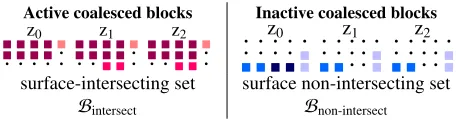
• When multiple surfacesare considered, the coalesce function will next be ap-plied to other sub-blocks (within the same parent block) that intersect with other surfaces. This seldom happens but it is possible if the surfaces are close.

• Finally, the coalesce function isapplied to inactive sub-blocks(within the same parent block) which do not intersect with any surface. The result for inactive blocks (coloured in different shades of blue) are shown in Fig. 5.

To summarise, coalescing is applied only to surface-intersecting parent blocks which are subject to decomposition. The sub-blocks contained within may intersect with one or more surfaces, or not intersect with any surface at all. After consolidation, the output contains both the original and merged blocks. Based on the sub-block and surface intersection status, the consolidated blocks may be arranged into two separate sets, B_intersect andB_{non-intersect}, as shown in Fig. 5. Surface intersecting merged blocks

(within surface-intersecting parent blocks) are placed inB_intersect. Non surface-intersecting merged blocks(within surface-intersecting parent blocks) are placed inB_{non-intersect}. Non surface-intersecting parent blocks are also appended to this. The coordinate ascent algorithm provides a method for merging cells (sub-blocks of mini-mum size) within the confines of a parent block. Coalesced sub-blocks must share the same label and form a rectangular prism.

3.3.1 Practicalities

Since the cell division lines are identical for all parent blocks of the same size, to avoid having to compute the sub-block centroids and dimensions repeatedly, the cell dimen-sions and local coordinates of each sub-block’s centroid (relative to the parent block’s minimum vertex) are stored in a look-up table and indexed by parent block dimen-sions to speed up computation.

Please do not cite

(10)

10 RAYMONDLEUNG

3.4 Block tagging: domain identification using surfaces

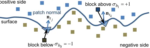
The primary objective is to label whether a block is located above or below a surface. A picture of this is shown in Fig. 6. More generally, the surface is not always horizontal, so it makes more sense referring to the space on one side of the surface aspositive, the other asnegative, however this is defined.

positive side

negative side block above

block below 1 0  b



1 1 b



surface

patch normal

j t

n ntk

Figure 6: Concepts relating to surfaces: surface normal (cross product) and block pro-jected distance (inner product) associated with a triangular patch

The main points to appreciate in Fig. 6 are that

• Each triangular patch of the surface has a normal vector associated with it. For example, the normalntk associated with triangletkpoints in the upward

direc-tion. This normal is computed by taking the cross product between two of its edges, for instance,(vk,1−vk,0)×(vk,2−vk,0). This arrow would point in the

opposite direction (rotate by 180o_{) if the edge traversal direction is reversed; for}

instance, by swapping two verticesvk,1andvk,2in the triangle.

• To determine “which side of the surface” a block is on, it suffices to consider the triangular patch located closest to the block. After establishing the positive side as the space ‘above’ the surface, one can say blockb1is located above the surface

and has a positive sign (σb1 = +1) because the inner product(ctk −cb1) ·ntk

is negative. Here, ctk andcb1 represent the centroid of triangletkand blockb1

respectively. Conversely, blockb0 is below the surface and has a negative sign

(σb0 =−1) because the inner product(ctj−cb0)·ntj is positive. This ‘projection

onto normal’ approach provides the first method for block tagging.

3.4.1 Discussion

For this method to work, the edges for each triangle in the mesh surface must be or-dered consistently (e.g., in the anti-clockwise direction) and any ambiguity in regard to surface orientation must be resolved to ensure the assigned labels ultimately con-form to user’s expectation — e.g., the positive direction points upward with respect to an open surface (or outward in the case of a closed surface).

www.josis.org

Please do not cite

(11)

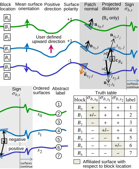
3.4.2 Labelling scheme: extension to multiple surfaces

This tagging logic may be extended to multiple surfaces. Fig. 7 depicts a multi-surface scenario and illustrates how abstract labels are assigned to multiple layers according to the truth table. Proceeding from left to right, blocks from seven distinct locations relative to the surfaces are shown. The mean surface orientation shows the direction obtained by averaging over all triangular patch normals. This arrow can point up or down provided the ordering of triangle vertices is consistent. Consistency can be enforced by ensuring triangle edges are traversed only in the anti-clockwise (or clock-wise) direction.

Thepositive directionis a user-defined concept. By default, it points in the upward direction (+z axis). For a vertical surface (e.g., a geological feature such as a dyke) that runs across multiple layers, the positive direction may be defined as left (or right).

Surface polarity indicates if there is agreement between the mean surface orientation (a property conferred by the mesh) and the positive direction (intention of the user). If they oppose, as is the case for the bottom surface in Fig. 7, the polarity is set to negative. The significance is that the interpretation of the projected distance between a block and relevant triangle, and subsequently what sign we assign to the block, depend on the surface polarity.

Focusing now on the shaded portion of Fig. 7, comparison of blockB4with surface

1 yields (cts1,j−cB4)·ns1,tj > 0, hence its sign σB4,s1 isnegative (it is below the s1

surface). However, comparison with surface 2 yields apositivesignσB4,s2 (it is above

the s2 surface) even though the projected distance(cts2,k−cB4) ·ns2,tk > 0; this is

correct sinces2has negative surface polarity which negates the logic.

Abstract labels are assigned to merged blocks to distinguish between boundaries and embedded layers. By convention, layers are given odd-integer labels whereas boundaries (the interface between layers) are given even-integer labels. For the inter-leaved layers, given its signσb,sn and affiliated surfacesn,

3_{the abstract label is given}

by λ(sn, σb,sn) = 2×(n+ 1)−σb,sn for n ≥ 0, where σb,sn ∈ {−1,0,+1} represent

{below, across, above} the surface, respectively.

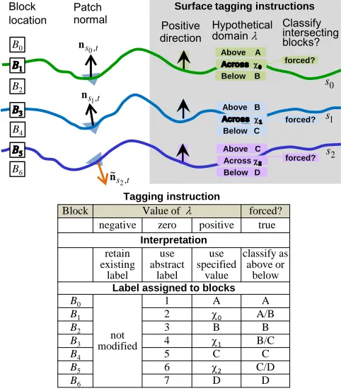
3.4.3 Tagging instructions

With block tagging, there is tremendous scope for creativity. The scheme described below provides a flexible framework for domain specification given arbitrary surfaces. The diagram shown in Fig. 8 is similar to Fig. 7 for the most part. What is different is the emphasis onsurface tagging instructions. Observe that there are three sets of tagging instructions: one for each surface. Each instruction specifies (1) a positive direction for each surface; (2) nominal labels for blocks located above, across and below each surface; (3) an override field (see “forced?”) which communicates an intent to either

preserve the surface intersecting blocks (by assigning a label different to any other

3_{Affiliated surface indices}_s

nare deduced from the columnσsnin the truth table. Refer to the

high-lighted cells for each block in Fig. 7

Please do not cite

(12)

12 RAYMONDLEUNG

Block

location Surface polarity Mean surface

orientation Positive direction Patch normal

Projected distance σSign b,s

t s₁,

n

t s2,

~

n

t s0,

n B1 B₂ B₄ B₅ B₆

B₀ ₊₁

+1

-1

(B4 only)

• B₃ >0 >0 j s

t1,

k s

t₂,

4

B

c

j

t s₁,

n

k

t s2,

n

block label

B₀ + + + 1

B₁ +/– + + 2

B₂ – + + 3

B₃ – +/– + 4

B₄ – – + 5

B₅ – – +/– 6

B₆ – – – 7

0

,s b

σ σb,s₁σb,s2

Truth table

Affiliated surface with respect to block location Ordered

surfaces Sign Abstract

label 0 s 1 s 2 s 1 2 3 5 6 7 • 4 s b, σ User defined upward direction surfaces continue surfaces continue positive negative

Figure 7: Block tagging in a multi-surface scenario: terminologies and truth table for the signs

layers) or resolve whether these blocks are strictly above or below the surface, i.e., force a binary decision.

A trivalent logic is built into the nominal labels specified in item 2. In Fig. 8, this is denoted by λ. User-specified values are assigned to blocks whenλ > 0. In addition, there are two special cases worth mentioning. First, an input value ofλ= 0instructs the program to use abstract labels instead of specific domain values (see “zero” col-umn in Fig. 8). Second, a negative input value λ < 0instructs the program toleave current labels intact. This retains any prior label which has been assigned to that block (see “negative” column in Fig. 8). This ‘retain existing labels’ mode allows the spatial structure of a block model to be updated without invalidating previous domain as-signments. For instance, a surfaces0may be used as an upper bound. Ifλ(above)s0 =−1,

then all blocks located above this surface will not have their labels modified. Similarly,

s1 may be used as a lower bound. Ifλ(below)s1 =−1, then all blocks located below this

surface will not have their labels modified.

www.josis.org

Please do not cite

(13)

Block Value of  forced?

negative zero positive true Interpretation retain existing label use abstract label use specified value classify as above or below Label assigned to blocks

B0

not modified

1 A A

B1 2 0 A/B

B2 3 B B

B3 4 1 B/C

B4 5 C C

B5 6 2 C/D

B6 7 D D Tagging instruction Block location 0 s 1 s 2 s t s1, n

t s2,

~

n

t s0, n

B2

B4

B6

B0

Surface tagging instructions

Positive direction

Above A

Below B

Above B

Below C

Above C

Below D

Hypothetical domain 

forced?

Patch

normal _Classify intersecting blocks?

Across 2

Across 1

Across 0

B1

B5

B3

Figure 8: Block tagging instructions: interpretation of the lambda value

3.4.4 Retaining existing domain labels

As a motivating example, suppose we rotate the picture in Fig. 8 counter-clockwise by 45 degrees. Further, suppose the entire block model is currently labelled as domain A. Then, the space between the two tilted surfaces (below s0 and above s1) can be

used to model a dolerite channel that runs diagonally across the layers. By using the following specification: λ(above)s0 = −1, λ

(below)

s0 = B, λ (above)

s1 = B, λ (below)

s1 = −1 and

forced(s) =TRUEfor both, blocks within the embedded layer will be tagged as domain

B (dolerite) for some B>0.

4

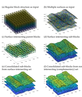
Visualisation

This section illustrates some of the results produced by the proposed framework. Fig. 9(a) shows a regular block structure which covers the regionx∈[1000,1250], y ∈ [750,925], z ∈ [590,670] with parent blocks measuring25×25×5m. Three horizon-tal surfaces are also given as input, these are shown in Fig. 9(b). Surface-intersecting parent blocks identified in (c) are subject to block decomposition. Using block-triangle overlap detection, the surface-intersecting sub-blocks, each measuring5×5×1m, are identified in Fig. 9(d). To reduce fragmentation, the decomposed sub-blocks in the

Please do not cite

(14)

14 RAYMONDLEUNG

(a) Regular block structure as input (b) Multiple surfaces as input

(c) Surface intersecting parent blocks (d) Surface intersecting sub-blocks

(e) Consolidated sub-blocks (f) Consolidated sub-blocks from non-from surface-intersecting set intersecting (complementary) set

Figure 9: Block restructuring given multiple surfaces

surface-intersecting and non-intersecting sets are consolidated in Fig. 9(e)–(f). For the surface-intersecting set, the block-count decreases from 8497 to 2102 after sub-blocks are coalesced.

In regard to theforcedoption for block tagging, the differences between preserving the boundary and classifying the blocks at the interface as strictly above / below a surface are demonstrated in Fig. 10(g)–(h). For clarity, Fig. 10(i) shows only blocks labelled as A and C (belonging to two domains of interest) in isolation. Clearly, they conform to the shape of the relevant surfaces. In Fig. 10(j), only blocks that intersect with the top surface (labelled 2) have been extracted.

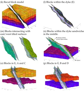
4.1 Iterative refinement: an application to tilted surfaces

The running example has thus far taken only a regular block structure as input. In this section, we demonstrate that the framework can also modify the spatial structure of a model with irregular (non-uniform) block dimensions. Of particular interest is that tilted surfaces are used to model a hypothetical dyke channel running through bedded

www.josis.org

Please do not cite

(15)

(g) Resolving boundary blocks (h) Preserving boundary blocks forced=1 classifies as above/below forced=0 maintains unique identity

1 (A)

3 (B)

5 (C)

7 (D)

1 (A)

3 (B)

2

4 5 (C)

7 (D)

6

(i) Isolated blocks from A and C (j) Localised blocks extracted from — two domains of interest the A/B interface

Figure 10: Block tagging given multiple surfaces

layers. This highlights two significant features: (a) ability to iteratively improve the spatial structure of an existing block model whilst preserving the labels for horizontal strata which have been previously assigned; (b) ability to work with oblique surfaces and produce correct result when the surface orientation is ambiguous (positive may not point upward), thus user has to specify precisely what is meant by the positive direction in relation to the supplied tagging instructions. An example of this is shown in Fig. 11.

  

 

  

 

  

4243 . 0

7071 . 0

5657 . 0

Tagging instructions Above E

Below -1

Second tilted surface s₁

First tilted surface s₀ Across 8

Positive direction

Forced? no

670

660

650

640

630

620

610

600

1050 1100 1150 ₈₀₀ 850 900

Below E Above -1

Across 10

Figure 11: Block tagging instructions for tilted surfaces

Please do not cite

(16)

16 RAYMONDLEUNG

(k) Recut block model (l) Blocks within the dyke (E)

(m) Blocks intersecting with (n) Blocks within the dyke sandwiched east/west tilted surfaces in the middle.

8 (abstract label)

crust of dyke surface

10

C D

E (dyke) (o) Blocks in E, A and C (p) Blocks in E, B and D

Figure 12: Iterative refinement incorporating tilted surfaces

Fig. 12 shows the recut block model follows the curvature of the tilted surfaces. In (k), blocks within the dyke are removed for clarity. Pre-existing labels (outside the dyke) remain intact. The spatial structure is only modified around the tilted surfaces. In Fig. 12(l)–(m), blocks within the dyke and those located on the east / west interfaces are shown in isolation. Fig. 12(n)–(p) show the existing labels for blocks in A, B, C and D have been perfectly preserved. As expected, new labels — {8, 10} and E respectively — have only been assigned to blocks that intersect with and sandwiched between the tilted surfaces.

5

Discussion

Critical reflection and user feedback are both essential to designing robust and flexible systems [2]. Guided by the principle of reflective and iterative design [19], there was an early and continued focus in our approach on real usage scenarios [18], as well as successive evaluation, modification and scenario-based testing. In this section, we

www.josis.org

Please do not cite

(17)

describe two improvements made to eliminate flaws identified through this process which made the system more robust.

5.1 Issue 1: Sign inversion due to sparse, jittery surface

positive side

negative side

k

t

n

j

t

n

surface triangle t_j

surface triangle t_k

Side-on view

+ –

block

Figure 13: Local sign inversion when triangle mesh surface is sparse and jittery

In regard to block tagging and ‘which-side-of-the-surface’ determination, the ‘projection-onto-normal’ method described in Section 2.4 works well when the sur-face is smooth and triangle mesh is dense and uniform. Potential issues arise when the surface exhibits local jitters and the triangles are sparse. For instance, the mesh resolution is low relative to the parent block size when triangle patches stretch over distances of up to one kilometer in certain areas. As an illustration, Fig. 13 shows a block associated with triangletj (the nearest patch based on block-triangle centroid-to-centroid distance). This association yields the wrong result, a negative sign with respect to the normal ntj is obtained (according to the plane partitioning test) even

though it lies above the surface. We observe the projection of the block lies outside the support interval of the referenced triangletj and the same comparison withtkwhich is further away would produce the right result (a positive sign). This problem can be remedied by upsampling the mesh surface to increase its density. Fig. 14 shows an ex-ample where triangles are recursively split along the longest edge until the maximum patch area and length of all edges fall below the thresholds of 1250m2 and 100m. A better solution, however, is ray-tracing. This recommended approach is described in Appendix B. The key advantage is that ray tracing is not susceptible to variation in surface mesh density (the sign inversion problem), furthermore, it does not require dense surfaces or consistent (e.g. clockwise) ordering of triangle vertices.

Before: non-uniform density After: high density mesh

Figure 14: Increasing mesh density of a real surface by splitting the longest edge of suprathreshold triangles recursively

Please do not cite

(18)

18 RAYMONDLEUNG

5.2 Issue 2: Boundary localisation accuracy

The block consolidation component, as it currently stands, considers the sub-blocks that belong to the surface-intersecting set (B_intersect) and non surface-intersecting set (B_{non-intersect}) independently. As Fig. 5 has shown, the sub-blocks (cells) within each respective set are merged separately to form larger rectangular prisms within the con-fines of the parent blocks. While this split is useful for extracting surface-intersecting sub-blocks, it has two drawbacks. In terms of boundary localisation accuracy, Fig. 15(a) shows that surface-intersecting sub-blocks — with centroids located on dif-ferent sides of the surface — are merged together irrespective of whether it is pre-dominantly above or below the surface. In terms of compaction,merging potential is limitedbecause adjacent cells fromB_intersectandB_{non-intersect}cannot be coalesced even if they lie on the same side of the surface.

To reinforce the first point, the two cells marked with “?” in Fig. 15(a) ought to be labelled as above the surface. However, under the current regime, they are considered jointly with the three cells immediately to the right that also intersect with the surface, thus they are treated collectively as a 1-by-5 merged block. Since the centroid (black dot) lies marginally below the surface, the merged block will also be labelled as such. This distorts the boundary as it introduces a vertical bias of around ∆(block)_y,min /2to the two left-most cells.

Surface-intersecting sub-blocks Non surface-intersecting sub-blocks

Consolidated blocks

below surface (a) proposed scheme in Section 3.3 (b) proposed scheme in Section 5.2

Hypothetical surface Sub-block

classification

above surface ? ?

  

 



   

centroid Domain

classification Tagging of

merged blocks merged blocks Tagging of

class 0

class 1

Figure 15: Treating surface-intersecting and non-intersecting sub-blocks,B_intersectand

B_{non-intersect}, independently during block consolidation may reduce boundary localisa-tion accuracy and limit merging potential. In the latest proposed scheme (Seclocalisa-tion 5.2), sub-blocks are classified by their location relative to the surface before sub-blocks con-solidation.

To accurately localise the boundary and achieve the result shown in Fig. 15(b), ray tracing is used to determine the location of cells with respect to each relevant surface that intersects the parent block. Given S surfaces, the {0=above (or no intersection), 1=below} decisions naturally produce up to 2S categories (or states) which would be treated separately during sub-blocks consolidation in lieu ofB_intersectandB_{non-intersect}.

www.josis.org

Please do not cite

(19)

In practice, however, we suggest encoding the location with respect to each surfaces

using 3 bitsb3s+2b3s+1b3s, where the mutually exclusive bits are set to 1 to denote the

outcomes ofabove,belowanduntested, respectively. The rationale is that whenb3s= 0, domain identification needs not be attempted during block tagging with respect to surfaces, since the decision has already been made here prior to sub-blocks consolida-tion (eitherb3s+2 = 1orb3s+1 = 1) and this information is passed on. In fact, applying

ray-casting at the cellular-level (highest resolution) yields more accurate results near the surface than applying to merged blocks, especially for undulating surfaces with high local curvature.

To summarise, administering ray-casting before sub-blocks consolidation helps di-vide cells along surface boundaries; this increases boundary localisation accuracy and ensures merging is performed within the right domains with maximum potential. Ta-ble 1 provides a comparison of the techniques discussed.

Raymond Leung/Ore Geology Reviews 00 (2019) 1–13 9

cation of cells with respect to each relevant surface that inter-sects the parent block. GivenS surfaces, the{0=above (or no

intersection), 1=below}decisions naturally produce up to 2S

categories (or states) which would be treated separately during sub-blocks consolidation in lieu ofBintersectandBnon-intersect. In

practice, however, we suggest encoding the location with re-spect to each surface susing 3 bits b3s+2b3s+1b3s, where the mutually exclusive bits are set to 1 to denote the outcomes of

above,belowanduntested, respectively. The rationale is that

whenb3s = 0, domain identification needs not be attempted during block tagging with respect to surfaces, since the de-cision has already been made here prior to sub-blocks consol-idation (eitherb3s+2 = 1 or b3s+1 = 1) and this information

is passed on. In fact, applying ray-casting at the cellular-level (highest resolution) yields more accurate results near the sur-face than applying to merged blocks, especially for undulating surfaces with high local curvature.

To summarise, administering ray-casting before sub-blocks consolidation helps divide cells along surface boundaries; this increases boundary localisation accuracy and ensures merging is performed within the right domains with maximum poten-tial. Table 1 provides a comparison of the techniques discussed. Fig. 16 illustrates block model spatial restructuring results ob-tained from a typical mine site.

Surface-intersecting sub-blocks Non surface-intersecting sub-blocks

Consolidated blocks

below surface

(a) proposed scheme in Section 3.3 (b) proposed scheme in Section 5.2

Hypothetical surface Sub-block classification above surface ? ?            centroid Domain classification Tagging of

merged blocks merged blocks Tagging of

class 0

class 1

Figure 15: Treating surface-intersecting and non-intersecting sub-blocks,

BintersectandBnon-intersect, independently during block consolidation may re-duce boundary localisation accuracy and limit merging potential. In the latest proposed scheme (Section 5.2), sub-blocks are classified by their location rela-tive to the surface before sub-blocks consolidation.

6. Block merging to reduce fragmentation

The proposed block merging algorithm can also be used to consolidate a fragmented block model that exists with or with-out reference to any mesh surface. Fragmentation is used in this context to mean a highly redundant block model representation where blocks near the boundary are over-segmented or divided in an excessive manner to follow the curvature of a surface with-out regard for the compactness (total block count) of the model. As an illustration, Fig. 17(b) shows a highly fragmented block model for theStanford Bunnycreated by block decomposition without consolidation. In an effort to closely approximate the

surface, numerous blocks at the minimum block size were pro-duced near the surface. Fig. 17(c) shows a clear reduction in

Techniques for ‘which side of the surface’ determination

•Projection onto normal method(Section 2.4)

+Ability to extrapolate boundary beyond surface support interval

– Susceptible to sign inversion problem depicted in Fig. 13

•Ray tracing method(Section 5.1 and Appendix B)

+Not impacted by sparse, jittery surface

+Consistent edge ordering in triangular mesh surface not required

– Result only defined over support interval of the supplied surface

Techniques for sub-blocks consolidation and boundary localisation

•Earlier proposal(Section 2.3)

– Limited block merging potential due to class segregation – Possible boundary distortion (introduce small bias)

•Latest proposal(Section 5.2)

+Classify sub-blocks w.r.t. surface before consolidation +Accurate (merge & label decisions made at highest resolution)

Table 1: Comparison of techniques with emphasis on system robustness

Figure 16: Typical block model spatial restructuring results. Top: blocks parti-tioned by surfaces into different domains (not all surfaces are shown). Bottom: reveals two block sets with different levels of mineralisation in an ore deposit. Zoom in to see individual blocks.

block density as blocks are appropriately merged. This results in a more compact block representation (3D segmentation) of the object.

The block merging algorithms are formally described in the Supplemental Material wherein a number of technical issues are discussed in depth. At its core, one noteworthy extension is that ‘feasibility of cell expansion’ is determined using a multi-valued, rather than boolean, 3D occupancy map, where the val-ues correspond to the identity of the cells or sub-blocks. The spatial constraints governing cell expansion are somewhat dif-ferent, in particular, the lateral dimensions orthogonal to the axis of expansion have to match for all the blocks involved in a merge. These, along with other relevant considerations and im-plementation details, are described in Appendix D.4–Appendix D.6.

Table 1: Comparison of techniques with emphasis on system robustness

5.3 Applications

Fig. 16 shows block model spatial restructuring results obtained for a typical mine site. In this example, surfaces were created to separate geological domains (mineralised, hydrated and waste) within the Brockman Iron Formation which contains members of interbedded BIF and shale bands in the Hamersley Basin Iron Province [5]. Al-though ore-genesis theories vary depending on the minerals or commodity, the abil-ity to model formations and features such as igneous intrusions in ore deposits is of general interest in areas not limited to mining, but also in further understanding the structural geology of mineral deposits. Using open and closed surfaces to represent structures of varying complexity — this may encompass volumes with exceptional geochemical or geophysical attributes — it is possible to extract waste pockets with

Please do not cite

(20)

20 RAYMONDLEUNG

high concentration of trace elements, or regions with magnetic / gravity anomaly [23]. Equally, if the surfaces represent the boundary of aquifers separated by clay and lignite seams [25], the process may serve as a basis for creating a structural hydrogeological model to study hydraulic and transport conditions in environmental risk assessment. The techniques developed for shaping a 3D block model can be used potentially in a variety of contexts.

Figure 16: Typical block model spatial restructuring results. Top: blocks partitioned by surfaces into different domains (not all surfaces are shown). Bottom: reveals two block sets with different levels of mineralisation in an ore deposit. Zoom in to see individual blocks.

6

Block merging to reduce fragmentation

The proposed block merging algorithm can also be used to consolidate a fragmented block model that exists with or without reference to any mesh surface. Fragmentation is used in this context to mean a highly redundant block model representation where blocks near the boundary are over-segmented or divided in an excessive manner to fol-low the curvature of a surface without regard for the compactness (total block count)

www.josis.org

Please do not cite

(21)

of the model. As an illustration, Fig. 17(b) shows a highly fragmented block model for the Stanford Bunnycreated by block decomposition without consolidation. In an effort to closely approximate the surface, numerous blocks at the minimum block size were produced near the surface. Fig. 17(c) shows a clear reduction in block density as blocks are appropriately merged. This results in a more compact block representation (3D segmentation) of the object.

(a) Stanford Bunny mesh surface

(b) Fragmented block model (c) Consolidated block model 187292 of 716773 blocks inside surface 435117 of 1217596 blocks inside surface

72027 vertices, 144046 triangles

Support interval X: [-1, 0.78] Y: [-0.02, 1.78] Z: [-0.58, 0.82]

Block origin: [-1, -0.02, -0.58] Parent block dimensions: [0.02, 0.02, 0.02] Minimum block size: [0.004, 0.004, 0.005]

Figure 17: Block merging applied to Stanford Bunny to reduce block fragmentation. Zoom in to see individual blocks.

The block merging algorithms are formally described in the Supplementary Ma-terial wherein a number of technical issues are discussed in depth. At its core, one noteworthy extension is that ‘feasibility of cell expansion’ is determined using a multi-valued, rather than boolean, 3D occupancy map, where the values correspond to the identity of the cells or sub-blocks. The spatial constraints governing cell expansion are somewhat different, in particular, the lateral dimensions orthogonal to the axis of expansion have to match for all the blocks involved in a merge. These, along with other relevant considerations and implementation details, are described in Appendix D.4–Appendix D.6.

Please do not cite

(22)

22 RAYMONDLEUNG

6.1 Merging conventions and optimisation objectives

The block merging algorithms also recognises that merging can be performed under different conventions. For example, in Algorithm 2, the procedure preserves the in-put block boundaries, it does not introduce new partitions (sub-divisions) that are not already present in a parent block. This merging convention is referred as persistent block memory. It has th