On a Numerical Algorithm for Uncertain System

ISSN 1597-6343

ON A NUMERICAL ALGORITHM

FOR UNCERTAIN SYSTEM

*ABIOLA,B. & IBIWOYE, A.

Department of Actuarial Science& Insurance, University of Lagos, Nigeria.

*_{[email protected]}

ABSTRACT

A numerical method for computing stable control signals for system with bounded input disturbance is developed. The algorithm is an elaboration of the gradient technique and variable metric method for computing control variables in linear and non-linear optimization problems. This method is developed for an integral quadratic problem subject to a dynamic system with input bounded uncertainty.

Key words: Stable Control, Gradient Technique, Variable Metric

Method and Input bounded Uncertainty.

INTRODUCTION

This paper is concerned with the development of a numerical method for the computation of controls for system with bounded input disturbances. Existing numerical methods for computing control signals for optimisation problems do not consider the situation when uncertainties are involved in the system, this work is set to give consideration to such problem and for a start we shall develop this method for an integral quadratic problem subject to a dynamical system with input bounded uncertainty.

Formulation of Problem:

Consider

Min





T

dt

t

Ru

t

u

t

Qx

t

x

0

{

(

)

(

)

(

)

(

)}

… (1)

subject to

)

(

)

(

)

(

)

(

t

Ax

t

Bu

t

Cv

t

x









… (2)

and

,

)

0

(

0

x

x



given,

t



[

0

,

T

],

… (3)

N

R

X

t

x

(

)





, is the state vector

u

(

t

)



U



R

M

is the control vector and

v

(

t

)



V



R

M is the uncertain vector.

.





V

U



T is the final time.

Q



R

NMis positive semi-definite (symmetric)

R



R

M is a positive definite matrix. We state the following assumptions:

1

A

: We assume that A is a stable matrix and if otherwise there exist a matrix

N M

R

K



 such that

A



A



B

T

K

.

Given that

PD

N denotes the set of positive symmetric members of

R

NN

Then

,

0

1







A

P

Q

A

P

T

Q

₁



PD

N … (4)

:

2

A

v

(

t

)

is a Caratheodory function and given

m

,

m

,

IR



m



v

(

t

)



m

:

3

A

(

A

,

B

)

,is controllable.

For our subsequent development of this paper, we now consider

)

(

)

(

t

Ax

t

x





… (5)

Let



(

t

₀

,

t

)

be a transition matrix for (5) then we can write the solution for equations(2) and (3) as











t

t

x

T

t

x

0 0 0

,

)

(

)

(

)}

(

)

(

)

,

(

t



Bu





Cv



d



… (6)

We calculate the transition matrix using the following formula





 























n

k

n

j i j

j k

I

A

f

A

f

1 1

)

(

)

(









… (7)

Where

k



denotes the eigen-value of the matrix A.

Let

B

[

IR

N

,

IR

M

]

be the set of bounded linear map between

N

IR

and

IR

M . We now define a map

]

,

[

]

,

[

:

B

IR

N

IR

M

B

IR

N

IR

M

L



Be such that







Bu

d

t

Lu

t

(

,

)

(

)

0







… (8)

And similarly define







t

t

Cv

Kv

0

(

,



)

(



)

d



… (9)

For arbitrary elements

w

₁

,

w

₂



IR

N, define the inner product on

IR

N as

dt

t

w

t

w

w

w

,

t

(

)

T ₂

(

)

0 1 2

1







… (10)

Ful

l Le

ngt

h

R

es

ea

rc

Let



(

t

₀

,

t

)

x

₀



z

₁ … (11)

Therefore

Kv

Lu

z

t

x

(

)



₁





… (12)

We can now write (1) as











(

),

(

)

(

),

(

)

)

,

(

u

v

x

t

Qx

t

u

t

Ru

t

J

=



z

₁



Lu



Kv

,

Q

(

z

₁



Lu



Kv







u

,

Ru



… (13)

Therefore,



































Kv

KQ

v

Qz

K

v

Lu

Q

z

Kv

LQ

u

Lu

KQ

v

u

R

L

LQ

u

v

u

J

T T

T

T T

T

,

,

2

2

,

2

,

)

(

,

)

,

(

1 ,

1

… (14)

We state the following remarks

Remark (1):

J

(

u

,

v

)

is convex with respect to

u



U



IR

M

Proof; Consider

0

)

,

,

(

]

)

(

,

[



u

LQ

T

L



R

u







Lu

LQ

T

u







u

Ru





This implies convexity.

Remark (2): Under the assumption that

u

(

t

)

is a minimizer for

J

(

u

,

v

)

and

v

(

t

)

is a maximizer , then

J

(

u

,

v

)

is concave with respect to

v



IR

M

Proof: Let



_i be

l



dimensional row vector of matrix

KQ

T

K

. Denote the norm of

v

by

v

. Since

v

is assumed bounded there exist

m

~

such that

v



m

~

. Now consider

0

]

[

)

(

,

2 2 2

2

1 2

1 2





















 

d

K

KQ

Tr

m

v

v

Kv

KQ

v

T

l

i i l

i i T

…(15)

Assumption:

4

A

: By Minimax theorem (Abiola, 2009) we assume

v

(

t

)





m

0

u

(

t

)

where

m



v

(

t

)



m

, and

).

(

2

1

0

m

m

m





Using

A

₄, we write

J

(

u

,

v

)

as























Qz

K

u

m

Lu

Q

z

u

L

KQ

m

m

R

L

LQ

u

u

J

T T

T T

,

2

,

2

)

)(

2

)

((

)

(

,

)

(

0 1

0 2 0

…(16)

We state the following proposition from (14).

Proposition (1)

For every

m

0



0

,

{(

LQ L

T



R

) (



m

o

)

2



2

m KQ L

o

(

T

)}



0

The prove of the above proposition is an obvious fact.

Numerical Method

The problem under consideration is the minimization of

J u

( )

defined in (16) with respect to the control signal

u t

( )



IR

n.

( )

J u

is non-linear, continuous and twice differentiable. We wish to find numerically

u

*

such that:

( *)

( )

J u



J u



u u u

:



*





Suppose



J u

( )

denotes the gradient of

J u

( )

, and we also set

( )

( )

J u

g u





… (17)

Let

2

( )

( )

J u

A u





… (18)

Where

A

(

u

)

denotes the Hessian matrix at point

u

.

we assume that

A

(

u

)

is non-degenerate at point

u

*. The first order condition for minimum is that

( )

0

J u





… (19)

A second order condition for minimum is that

2

( )

( )

0

J u

A u







… (20)

We see from proposition (1) that

A x

( )



0

One way of minimizing an unconstrained optimization problem is by application of Newton’s Method, which is described briefly below:

We consider the problem described as:

Min

F

(

x

),

x



IR

n … (21)

Find

x

*

such that



x

*

x



x





and

F x

(

*

)



F x

( )

.

Suppose



F x

( )



g x

( )

is the gradient of

F x

( )

at point

x

and



2

F x

( )



A x

( )

is the Hessian matrix, then the function

( )

F x

at each iteration is approximated by a quadratic model



and effectively minimized as:

1

(

)

( )

( )

(

( ) )

2

T T

x

p

F x

g x

P

P A x P











… (22)

Using the first order condition for minimum, we have

(

x

p

)

F x

( )

A x P

( )

0







 





… (23)

Solving equation (23) we have

)

(

)

(

x

p

F

x

A





… (24)

On the basis of (24) we state the Newton’s Algorithm.

Newton’s Algorithm

Step 1 Calculate

F

(

x

_k

).

g

(

x

_k

),

A

(

x

_k

)

Step 2. Check if

g

(

x

_k

)





for a predetermined



,

if so stop, else

Step3. Set

A

(

x

_k

)

P

_k=



g

(

x

k

)

Step4. Set

x

_k1



x

_k



P

_k

Step5. Set

k



k



1

,

and go to Step1.

The Newton’s algorithm described above can be shown to have second order convergence (Dixon, 1975). This is because it utilizes quadratic model which is minimized at each iteration. The global convergence of Newton’s method is not guaranteed because the iteration

can diverge from arbitrary starting points. Since Newton’s equations have to be solved at each iteration, it breaks down when

A

(

x

k

)

is

singular. However, to circumvent the drawback posed by the possibility of singularity of

A

(

x

_k

)

, a variable metric algorithm was proposed (Dixon, 1975)

The scheme involves the following:

)

(

1 k

k k k

k

x

P

g

x

x

_







… (25)

0 0

,

P

x

are guessed arbitrarily.



_k is determined by a suitable line search method.

P

0is a positive definite matrix and normally

P

k is intended to be approximation of the inverse of the Hessian matrix



2

F

(

x

)

.

This matrix is updated using information obtained in each iterative step as follows:

)

,

,

,

(

1 k k k k

k

z

y

v

P

P





… (26)

Where

v

k



x

_k1



x

_k,

y

k



g

_k1



g

_k

,

and

z

k is a vector parameter.

Variants of the variable metric algorithm are derived in the way in which the appropriate inverse matrices are constructed. A lot of methods

for determining

P

khave been proposed. For example (Dixon, 1975) proposed an updating rule for

P

k such that

D

P

P

k1



k



… (27)

where D is required to be very small as much as possible in some norm. He suggested the following Frobenious norm, defined as:

]

[

2 _T

D

W

D

W

Tr

D







… (28)

W

is a positive definite matrix.

D

is assumed symmetric such that

0





D

D

T … (29)

The quasi-newton condition defined as:















y

P

W

r

r

Dy

k

0

… (30)

is also satisfied.

Minimising (28) subject to (29) and (30) using Lagrange method an analytical solution for D was derived as:











T

T T

y

b

Py

W

b

Py

w

D



{

(





)



(





)

}

… (31)

where

,

1

y

W







y

W

y

Py

y

W

y

b

_T

T T

1

)

(

2

/

1







We next consider a method for constructing an approximation inverse for the Hessian matrix which also takes into consideration the uncertainty nature of the problem under investigation. This is the crux of this paper.

Minimising Algorithm

Consider the problem defined in (1) – (3) and let

))

(

)

(

)

(

(

)

(

)

(

)

(

)

(

)

,

,

,

(

x

u

v

x

t

Qx

t

u

t

Ru

t

Ax

t

Bu

t

Cv

t

H





T



T





T





…. (32)

be the system Hamiltonian.

Compute the gradient of (32) with respect to

u

(

t

)

as follows:

)

,

,

,

(

x

u

h

v



H



=

x

(

t

)

T

Qx

(

t

)



(

u



h

)(

t

)

T

R

(

u



h

)(

t

)





T

(

Ax

(

t

)



B

(

u



h

)(

t

)



Cv

(

t

))

. . . (33)

Since R is symmetric then

R

T



R

Therefore,

Bh

Rh

t

u

v

u

x

H

v

h

u

x

H

(

,



,

,



)



(

,

,

,



)



2

(

)

T





T … (34)

Now,

B

R

t

u

h

v

u

x

H

v

h

u

x

H

T T

h

















2

(

)

)

,

,

,

(

)

,

,

,

(

lim

₀ … (35)

Therefore

B

R

t

u

u

H

T T











)

(

2

… (36)

We now choose



(

t

)



2

Px

(

t

)

… (37)

P is a positive definite matrix calculated from (4), we then have

))

(

)

(

(

2

u

t

R

B

Px

t

u

H

T T









… (38)

This is expressible as

































H

u

u

t

R

BP

T

t

t

x



t

t

Bu

d

m



t

t

Cu

d

0 0

0

0

,

)

(

,

)

(

)

(

,

)

(

)

(

)

(

2

)

(













…(39)

We can now propose the following algorithm:

Define

J

(

u

)

by equation (16),



H

(

u

)

by (39), then

Step 1: Choose

u

₀ arbitrarily and compute

J

(

u

0

)

,



H

(

u

0

)

and set

k k

g

u

H





(

)

, and set

g

k





F

k

,

k



0

Step 2: If

g

_k





,

for a predetermined



,

stop, else set

Step 3:

u

_k1



u

_k





_k

W

_k

F

_k

(

u

_k

),

where











k k

k k k

F

A

F

g

g

,

,



A





(

LQ

T

L



R

)



((

m

0

)

2



2

m

0

)(

KQ

T

L

)







2

1

0

1 1

)

(

)

(





















t

k k

k

d

u

H

P

u

H

P

W



To avoid the possibility of

W

_k being negative definite, P is a positive definite matrix calculated from:

0







A

P

Q

PA

T

Updating of sequences is by gradient technique, which is defined as follows:

k k k

k

g

A

F

g

1







k k k

k

g

F

F

_1





_1















 

k k

k k k

g

g

g

g

,

1 , 1



Step 4: Set

k



k



1

and go to step 1

The convergence of this algorithm is similar to conjugate gradient algorithm given by Ibiejugba & Abiola (1985)

In what follows we show the procedure to derive the operator

W

_k

Suppose at iteration

k

and

k



1

k k

k

u

u

u

_1







… (40)

Let

S

(

u

)

be such that



































T

u

_k

t

dt

u

H

u

S

0

(

)

)

(

… (41)

where

H

(

u

)

u

H





















which was defined in (39)

Let a distance function be defined between

u

_k1 and

u

_k as follows:





S

)

T

(

u

_k

)

P

(

u

_k

)

d

(

0

2









… (42)

P

is a positive definite matrix calculated as before. We consider only when

,

0



S



and suppose there is an infinitesimal change in



u

_k which is defined as



d

ds

u

d

P

ds

u

d

T k k



















0

)

(

)

(

=1 … (43)

Then the corresponding change in (41) is given as



d

ds

u

d

u

H

ds

u

dS

T k T











































0

)

(

)

(

… (44)

We now minimise (44) by choosing

ds

u

d

(



_k

)

as control. In doing, this we use the

Lagrange multiplier technique and let



be the multiplier such that:







d

ds

u

d

P

ds

u

d

ds

u

d

u

H

S

T k T k k

T











































































0

)

(

)

(

)

(

… (45)

We define the Hamiltonian as follows:







































































ds

u

d

P

ds

u

d

ds

u

d

ds

u

d

u

H

H

k k T k k

T

)

(

)

(

)

(

)

(



 … (46)

ds

u

d

P

u

H

ds

u

d

H

_{T k}

k

)

(

2

)

(





























 … (47)

Setting (47) equals to zero implies

0

(





















ds

u

d

H

k  … (48) Therefore,

u

H

P

ds

u

d

_k









1

2

1

)

(



… (49)

Using (49) in (43) we have:





2

2 1 0 1



















































d

u

H

P

u

H

T … (50) Therefore 2 1 0 1 1

















































































  T k

d

u

H

P

u

H

u

H

P

ds

u

d



… (51) Numerical Illustration

Following Corless & Leitmann (1981), consider the following system defined by:















)

(

)

(

)

(

)

(

)

(

)

(

2 2 1 2 2 1

t

v

t

u

t

x

t

x

t

x

t

x





… (52)

The objective function is defined as

Minimize

J

u

v

x







u

(

t

)



u

(

t

)



dt

2

1

)

,

,

(

22

2 1

From the above, it is easy to see that



























2

1

0

0

2

1

R

,

















1

0

C

B

and

















0

1

1

0

A

We also note that

A

is unstable. We therefore select

K





k

₁

k

₂



such that

k

₁



0

,

k

₂



0





















2

1

1

0

k

BK

A

A

Let



Then if

0







A

P

Q

A

P

T , we can compute

































 

1 2 1 2 2

2

1

2

1

2

1

k

k

k

P

Suppose

2

1

2





k

then,



























2

2

1

2

1

2

P

which inverse is computed to be:































15

8

15

2

15

2

15

8

P

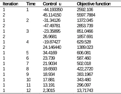
Applying the proposed algorithm, we have Table 1:

TABLE 1. CONTROL AND OBJECTIVE FUNCTION

Iteration Time Control u Objective function

1 1 -44.193350 2592.106 2 45.114150 5597.7884 1 2 -31.34126 1372.045 2 -47.49781 2853.739 1 3 -23.35895 851.0466 2 26.9681 1857.691 1 4 -19.87427 629.528 2 24.146440 1389.023 1 5 34.4169 606.081 1 6 23.739 587.460 1 7 21.9034 502.018 1 8 19.6593 422,2720 1 9 18.934 383.1967 1 10 17.881 343.480 1 11 13.191 296.097 1 12 2,3015 13,71743

Conclusion

We achieve the minimum of the objective function in just 12 iterations which can be considered as good enough. In our subsequent paper we shall consider the application of this algorithm water quality control system where uncertainties are involved. Furthermore we have demonstrated in this paper that it is possible to derive a numerical algorithm for some class of control problems where uncertainties are involved.

REFERENCES

Abiola, B. (2009). Control of Dynamical System in the Presence of Bounded Uncertainty. Ph.D Thesis, Department of Mathematics, University of Agriculture Abeokuta

Corless. M. & Leitmann, G. (1981). Continuous State Feedback Guaranteeing Uniform Ultimate Boundedness for Uncertain Dynamical System.IEE Transaction on Automatic Control, AC-26 No 5.

Dixon, L. C. W. (1975). On the Convergence of the Variable Metric Method with Numerical Derivatives and the Effect of Noise in the Function Evaluation, Optimization and Operation Research, Springer Verlag, Heidelberg, New York.

Ibiejugba, M. A. & Abiola, B. (1985). On the Convergence Rate of the Conjugate Gradient Method. AMSE Periodical, Advances in Modelling and Simulation, 2:21-31.