New Zealand Journal of Ecology(1994)18(2):123-168 ©New Zealand Ecological Society Landcare Research - Manaaki Whenua, PO Box 69, Lincoln, New Zealand.
1. Department of Science, Central Institute of Technology, Private Bag 39807, Wellington, New Zealand. 2. Botany Department, University of Otago, PO Box 56, Dunedin, New Zealand.
THE VEGETATION OF SUBANTARCTIC CAMPBELL ISLAND
__________________________________________________________________________________________________________________________________Summary:The vegetation of Campbell Island and its offshore islets was sampled quantitatively at 140 sites. Data from the 134 sites with more than one vascular plant species were subjected to multivariate analysis. Out of a total of 140 indigenous and widespread adventive species known from the island group, 124 vascular species were recorded; 85 non-vascular cryptogams or species aggregates play a major role in the vegetation. Up to 19 factors of the physical environment were recorded or derived for each site. Agglomerative cluster analysis of the vegetation data was used to identify 21 plant communities. These (together with cryptogam associations) include: maritime crusts, turfs, megaherbfields, tussock grasslands, and shrublands; mid-elevation swamps, flushes, bogs, tussock grasslands, shrublands, dwarf forests, and induced meadows; and upland tundra-like tussock grasslands, tall and short turf-herbfields, bogs, flushes, rock-ledge herbfields, and fellfields.
Axis 1 of the DCA ordination is largely a soil gradient related to the eutrophying impact of marine spray, sea mammals and birds, and nutrient flushing. Axis 2 is an altitudinal (or thermal) gradient. Axis 3 is related to soil reaction and to different kinds of animal influence on vegetation stature and species richness, and Axis 4 also appears to have fertility and animal associations.
Autecological interpretation of the data demonstrates clear niche segregation of congeneric species and species with similar growth forms. The notable megaherbs and giant tussocks may be an adaptation to harvesting nutrients from the aerosol precipitate. Heat harvesting in the cool, cloudy, wet, and windy climate may also be implicated. The history of farming and natural disturbances has resulted in a complex mosaic of vegetation-soil systems of varying maturity. Their putative dynamic interrelationships are depicted in terms of impacts of burning, grazing, marine animals and climate change and subsequent recovery or primary and secondary succession.
__________________________________________________________________________________________________________________________________
Keywords:Campbell Island; subantarctic; vegetation; environment; ordination; cluster analysis; tussock grasslands; tundra; scrub; dwarf forest; maritime communities; niche differentiation.
Introduction
Campbell Island (11 331 ha) is an isolated superoceanic, peat-covered island with numerous smaller offshore islets and stacks (Fig. 1), lying 700 km south of the New Zealand mainland at
52°33.7’S, 169°09’E (Clark and Dingwall, 1985; Meurk and Given, 1990). Extreme wind, cloudiness, high humidity, uniform cool temperatures (De Lisle, 1965), and soil fertility patterns (Campbell, 1981; Foggo and Meurk, 1983) establish the environmental gradients that influence vegetation patterns. The altitudinal range is from sea level to 558 m, which corresponds to mean January air temperatures of 9.3oC and 5.5oC respectively (Meurk and Given, 1990). Grounds for classifying Campbell Island as subantarctic are given in Meurk (1984). Domestic sheep and cattle, feral since the 1930s, were progressively eliminated between 1970 and 1990 (Dilks and Wilson, 1979; Rudge, 1986). Vegetation recovery from the
farming and grazing era has been especially marked on more fertile sites or where there are abundant seed sources (Meurk, 1982, 1989). Thus, at the time of this study there was a mosaic of near-pristine, reduced, induced, and heavily modified/grazed vegetation. This presented a more complex and disrupted pattern (Meurk and Given, 1990) than exists on the other southern islands of New Zealand.
There have been numerous accounts of the plants and vegetative cover of Campbell Island since the first serious observations recorded by Hooker (1844). These general references are listed in Godley (1965, 1970, 1979, 1989). The only systematic descriptions of the vegetation are those of Cockayne (1904, 1909, 1928) and Oliver and Sorensen (1951).
Figure 1:Simplified vegetation map (A) of Campbell Island, with locations of 140 vegetation sampling sites. The central boxed area is expanded as Fig. 1B (opposite). The base map and map unit symbols are derived by amalgamating related vegetation polygons from the original 1:25 000 map (Meurk and Given, 1990). Symbols used for the sample sites are coded according to their cluster analysis community type, with the letters referring to dominant species/growth forms (A =ChionochloaAntarctica, B =Bulbinella rossii, C = Coprosmashrubs, D =Dracophyllumspp., E = maritimE, F =Fellfield, G = meGaherbfield, H = Herbfield, I =Induced/grazed, J =Marsippospermum andJuncusspp., K =RostKovia magellanica, L =Poa Litorosa, M =Myrsinedivaricata, N =Nest sites, O = Poa fOliosa, P =Pteridophytes, Q =Hebe elliptiCA, R = Rock, S =Sedge, T =Turf, U = cUshion bog, V = Various slips/tracks, W = sea elephantWallow, X = eXotic/adventive plants, Y = non-vascular crYptogams, Z = bare peat -Zero vegetation).
Legend
Map Units
Tundra mosaic
Poa litorosameadow and Chionochloa
Maritime complex
Coprosma,slips and slumps
Cushion bog
Dracophyllum shrubland/dwarf forest
Edward Islands; Greene, 1964, and Smith and Walton, 1975, for South Georgia; Smith, 1972, for South Orkney Island; Davies and Greene, 1976, for the Crozet Islands). Recently some numerical classifications have been performed on aquatic communities of Macquarie Island (Hughes, 1986). In most of these studies, environmental records were used only to infer cause of the vegetation pattern. Multivariate analysis has been employed to quantify these relationships in preliminary results (Meurk and Foggo, 1988) and a restricted analysis from the Auckland Islands (Leeet al., 1991).
The vegetation pattern of these southern islands has a circumpolar unity, but the various elements are more or less well developed depending on latitude, isolation, age of substrate, and size of the landmass. Substrate fertility, as influenced by animals or maritime exposure, is also implicated (Smith and French, 1988). Wace (1960) and Bliss (1975, 1979) have attempted an integrated biogeographic classification for the circumpolar region. The main vegetation components are:
littoral-fringe and submaritime zones of cryptogams, cushion, and turf species; eutrophic maritime tussock grasslands commonly associated with giant herbs; scrub or dwarf heath-like forests where there is sufficient warmth and shelter; oligotrophic hard-cushion bogs; eutrophic sedge swamps; mesotrophic inland tussock grasslands; and upland rushlands, wet cushion bogs, turf grasslands, or cushion fellfields (see Meurk and Given, 1990, and Infomap 260, 1991; Plates 1-4, pp. 126, 131).
This paper quantifies the vegetation-environment pattern for Campbell Island using multivariate statistical analysis. We see merit in expressing the complexity of vegetation in terms of both community and continuum concepts.
Methods
Sampling the vegetation
The difficulties of collecting adequately representative data in remote field situations are exacerbated by limitations of time and weather conditions. Our compromise was to stratify the vegetation and sample according to the 30
physiognomic categories (formations) of Meurk and Given (1990). Aproximately 100 samples taken in 1980-81 (by CDM and MNF) were supplemented by previous records from 1970-1975 (CDM) giving an overall total of 140. Of these, six sites with less than two vascular species were excluded from analysis.
Samples were spread evenly through vegetation and geographic space (Fig. 1). The approach, when working a catchment, mountainside, or other physiographic feature, was to cover the range of vegetation categories, usually by sampling at regular intervals along some gradient, but also including unusual or rarely seen associations. The northern, sheep-free half of the island was sampled more intensively in order to represent less modified vegetation (Meurk, 1982, 1989). Of some 140 indigenous and widespread adventive vascular species known from the islands, 134 appeared in the samples. Of these, 18 species were excluded from analysis, largely because they occurred only once. In addition 85 non-vascular cryptogams (or aggregates) were recorded.
Sample boundaries and sizes were flexible, but defined limits were imposedbeforerecording commenced. Sampling was subject to the following constraints:
ï the general location was chosen from some distance, or was predetermined at some regular interval along a gradient;
Plate 2: A sheltered maritime cove (Davis Pt) with luxuriant megaherbfield, up to 1 m tall, ofStilbocarpa polaris, Anisotomelatifoliaand a head ofPleurophyllumspeciosum with shrubs ofHebe ellipticaand the fernBlechnum durum against the rock wall (CT 1).
Sampling the physical environment Altitude (m) - measured at each site using a
calibrated altimeter.
Slope (°) - microtopographic slope of the site was measured using an Abney level held on a rod, 1.5 m long, laid on the ground/vegetation surface down the maximum slope. Radiation (Langleys day-1) - mean daily net
radiation was derived from aspect, slope, and latitude using the method of Revfeim (1982). Distance to open coast (km) - distances to the
nearest open-sea coast were either estimated in the field or taken from a 1 : 250 000 map. Values were log transformed for statistical analysis.
Distance to any coast (km) - this differed from the above, when the nearest shoreline bordered an inlet or harbour.
Shelter (°) - angular elevation to the true westerly horizon (the source of the prevailing wind) was measured using an Abney level. Negative angles were recorded as zero.
Wind speed (m s-1) - site windspeed was recorded using a hand-held cup anemometer. At the beginning and end of each site observation, six wind speeds were recorded at 10-second intervals, and the mean calculated (Sws). This was corrected to long term January wind speed in the following way. Standard January wind speed on the Beeman Meteorological Station (Bws) anemograph (1970-1979, based on Reid, 1982) is 8.5 m s-1. Hand anemometer readings were found to be 0.52xanemograph readings. Then, corrected site wind speed = Sws/Bwsx 0.52x8.5 m s-1.
Soil temperature (°C) - site soil temperature (St) was measured (+/- 0.l°C) at 100 mm depth using an equilibrated electronic probe, and corrected in the following way. Long term mean January air temperature at Beeman Point is 9.3°C (N.Z. Met. Service, 1973). The mean of 25 days of 3 hourly, 100 mm soil
temperature readings was 0.8°C greater than mean air temperature ((max+min)/2). Plots of the daily soil temperature curve from Beeman Point allowed extraction of the Beeman soil temperatures (Bt) synchronous with St. Thus long term January soil temperature at the field sample site is (St-Bt) + 0.8 + 9.3°C.
Soil moisture (% of dry weight) - determined for the 50-100 mm depth section from a 45-mm-diameter soil core, oven-dried for at least 24 hours.
Soil depth (m) - was the mean of five measurements using a thin steel probe 1.5 m long. Soils deeper than this were recorded as 1.5 m. For • the vegetation stand was relatively large,
physiognomically homogeneous, and ideally part of a broad zone, and the site was
physiographically uniform;
• contiguous samples were avoided except on steep gradients, such as just above the littoral zone; • a formation was sampled only once within
approx. 2 km except where pre-established plots were used;
• each formation was limited to 3-6 samples. In some instances where the microtopography formed a fine-scale mosaic a sample was defined which encompassed this variation. However, identifiable parts of such mosaics were usually treated as separate sampling entities even if these were irregular in shape or made up of several disjunct bits. From previous experience (Meurk, 1982; Smartt, Meacock and Lambert, 1974) it appears that either presence/absence (P/A) data or crude quantitative data give an adequate
representation of a stand.
The following procedures were employed at each site.
• All species1were listed, with the top 10 or so in order of relative abundance.
• The average live vegetative height of each species was recorded according to a Raunkiaer-like, logarithmic progression of growth-form categories (Table 1).
• The cover was estimated for each species. • A biomass index number was derived from the
matrix (Table 1). This is the quantitative value used in subsequent analyses, and approximates a log transformation of absolute biomass. • At all sites thorough collections were made of
non-vascular cryptogams.
_____________________________________________________________
1Nomenclature for vascular plants follows Allan (1961),
Table 1:Symbols displayed on the 2-way table to indicate stature/cover estimates for each species less than 10 m. The quantitative values used in the multivariate analyses range from 15 (symbol “0” in table) to 1 (symbol “-”). The symbols #, *, +, =, - are biomass indices of decreasing value. The height class symbols imply approximation to Raunkiaer’s (1934) Microphanerophytes, Nanophanerophytes, Chamaephytes and Hemicryptophytes.
__________________________________________________________________________________________________________________________________
Cover description and upper limit of cover classes (%)
Dominant, Abundant, Frequent Common, Fairly Occasional, Sparse, Uncommon, Rare, Very Height classes very abundant, open all fields common, some fields 1 field requires 2 or 3 rare, 1
(m) continuous of view most fields search seen seen
__________________________________________________________________________________________________________________________________
M1= 2.5-10.0 0 9 8 7 6 5 4 3 2 1
N2 = 0.63-2.5 9 8 7 6 5 4 3 2 1 #
N1 = 0.16-0.63 8 7 6 5 4 3 2 1 # *
C2 = 0.04-0.16 7 6 5 4 3 2 1 # * +
C1 = 0.01-0.04 6 5 4 3 2 1 # * + =
H = 0-0.01 5 4 3 2 1 # * + =
-Cover class upper 100 75 50 25 12 5 2 1 0.5 <0.3
limit (%)
__________________________________________________________________________________________________________________________________
the shallow and variable mountain mineral soils, the mean was based on 10
measurements.
Redox potential (mv) - measured using an Orion portable specific ion meter with a platinum electrode that was inserted into the peat, and an Orion double-junction reference electrode (as described by Lee and Gibson, 1980). Readings were taken at 5 minute intervals until they had stabilised.
Soil samples to 150 mm depth were air-dried before storage and then analysed in Wellington within 2 months of collection. The samples were ground, including organic material and twigs of diameter less than 5 mm, but not sieved. The following measurements were made on this material. Soil pH - was measured by the method of
Blakemore, Seale and Daly (1977), except that the ratio of distilled water to soil was increased to 10:1.
Soil Ca, Mg, Na, K (mg cm-3) - cation levels were measured by atomic absorption
spectrophotometric analysis of ammonium acetate extractions (Blakemoreet al., 1977). The extracted solutions were measured three times, and the mean was corrected for bulk density of the original soil.
Soil conductivity (mmho) - determined in a conductivity cell (Blakemoreet al., 1977). Growth index (scale of 0-5) - from bioassay data of
Campbell Island soils (Foggo and Meurk, 1983) significant linear regression equations were derived for growth (of two species) against each of pH, Ca, Mg, and Na levels. These equations were used to predict bioassay growth for each of the sample soil pH, Ca, Mg, and Na levels. These eight values (after scaling the data from the two bioassay species) were
averaged to give a soil growth index for each sample site.
Animal index (scale of 0-5) - grazing influence was estimated by recording the cover of sheep pellets (infrequently cowpats), combined with the lowest height class of the biomass matrix. Other records - a subjective vegetation category was
applied to each of the sample sites (Fig. 1 legend). A photograph was taken at each site (Figs. 3-6), and the locality mapped (Fig. 1) to permit relocation of the sample site for comparative studies.
Vegetation analyses
The sites were classified into vegetation groups on the basis of the quantitative vascular species information using Cluster Analysis (Sneath and Sokal, 1973). The sorting strategy was flexible (beta = -0.25). The measure of dissimilarity was City Block. An inverse classification of the species into ecological groups, on the basis of their co-occurrences in the stands, was performed using similar methods, but with double-zero matches excluded (Sneath and Sokal, 1973). Although Cluster Analysis is a fusing method, it is convenient, for interpretation, to work top-down, and the distinctions are therefore described here as splits. The normal and inverse clusters have been ordered to conform with Axis 1 of the Detrended Correspondence Analysis within the constraints of the dendrogram (Tables 2, 3, Fig. 2).
Differences in environmental factors between groups from the vegetational classification were tested by the non-parametric Mann-Whitney Test (Snedecor and Cochran, 1967). Ordination of stands and species was performed by Detrended
G Anisotome antipoda- exposed summit tundra cushions, turfs, ferns, and forbs of shallow, fairly fertile soils;
H Poa annua- weedy herbs of grazed, maritime to flushed, fertile, shallow soils;
I Histiopteris incisa- localised ferns and mat forbs, often grazed and fertile;
J Hypolepis amaurorachis- an uncommon fern of lowland, deep, well drained soils;
K Cardamine depressa- localised on fertile shallow soils of maritime cliff crests; L Ranunculus subantarcticus- with G and Z the
main obligate tundra cushions and forbs, usually of low cover in fellfields and ledges, on gentle, sheltered slopes with shallow soils; M Sagina procumbens- scarce on mild, fertile,
disturbed or bird nest sites.Isolepis
praetextata- rare on saline, steep coastal rocks; N Cardamine subcarnosa- upland rush-herbfield
forb;
O Chiloglottis cornuta- orchid of lowland, sheltered shrublands on deep acid soils; P Lycopodium fastigiatum- components of
inter-tussock/shrub short grazed turfs on fertile soils.
Lyperanthus antarcticus- orchid of lowland, acid cushion bogs;
Q Lycopodium varium- dwarf forest epiphytes, ground ferns, and sedges associated with deep, infertile soils;
R Oreobolus pectinatus- cushions and forbs of lowland, gently sloping, exposed and grazed, deep acid bogs.
Eutrophic maritime herbaceous dominants: S Poa foliosaandAnisotome latifolia- dominants
of enriched, ungrazed, sheltered megaherbfield-grassland on steep, maritime slopes.
Dominant tussock grass and summer-green lily of mesotrophic to eutrophic grassland:
T Poa litorosaandBulbinella rossii- ubiquitous dominants of maritime and upland grazed tussock grasslands.
Dominant tussock grass of low altitude oligotrophic and middle altitude mesotrophic sites:
U Chionochloa antarctica- dominant tussock grass of ungrazed, deep acid soils on exposed slopes.
Eutrophic sedge-swamp dominants: V Carex appressaandBlechnum“sp.2”
-dominants of sheltered, lowland, fertile sedge swamps.
Largely oligotrophic to mesotrophic, middle to high altitude, open-space graminoids, forbs, mats, and cushions:
W Uncinia hookeri- ubiquitous matrix graminoids and forbs of upland grasslands, herbfields, and tall rushlands, including taller
Multiple regressions of the position of stands on the stand ordination were calculated against the environmental variables.
Results
Inverse Cluster Analysis (the species groups) Twenty-seven main vascular plant groups were derived from the inverse cluster analysis (Fig. 2, Table 2). The ecological significance of these groups is elucidated from the positions of the individual species and their clusters within the DCA ordination diagrams (Figs. 7, 8), the axes of which have been environmentally characterised by multiple regression and by single-factor mapping (Figs. 11-17).
The individual ecological groups or guilds are characterised by average environmental values, derived from the concentration of occurrences within site groups (Appendix) and their attributes (Table 4). Some of the groups are coherent in that the environmental range is narrow and can be clearly segregated as low, medium, or high in one or more parameters. Other groups comprise widely distributed opportunistic species or mixtures of infrequently occurring species, with consequent poor guild definition. The coherent groups are those with specialised species that are confined to stressful environments such as the littoral fringe, acid cushion bogs, swamps, or exposed summit ridges. The following lists sketch out the broad growth form and habitat attributes of the species clusters. The signature species indicated are those within the cluster which attain the greatest biomass index (Tables 2, 3).
Vascular plant groups
Mesotrophic to eutrophic, middle to low altitude and maritime turf, megaherbfield, grassland and shrubland species:
A Puccinellia chathamica- common littoral fringe cushions and turfs of shallow, fertile soils; B Hebe elliptica- maritime associates; C Stilbocarpa polaris- sheltered, ungrazed
rocks/ledges throughout;
D Poa ramosissima- seral or disclimax coastal grass on well drained, deep, acid soils often associated with bird colonies;
E Callitriche antarctica- mainly adventive grasses and forbs of coastal wet/flushed, shallow but fertile ground associated with animal disturbance;
F Pleurophyllum criniferum- herbs of sometimes grazed fertile swamps/flushes.
MarsippospermumandHierochloe brunonis
confined to high altitude rushlands;
X Juncus scheuchzerioides- medium turfy rush, common on non-maritime, mesotrophic/ flushed, wet, often gently sloping, eroded sites; Y Isolepis aucklandica- ubiquitous turfs or mats
of infertile gentle surfaces;
Z Rostkovia magellanica- cushions, forbs, and turf rush typically of exposed, high altitude shallow acid bogs; the palatablePleurophyllum hookeriflourishes only in the absence of grazing.
Scrub and dwarf forest dominants:
ZA Dracophyllum scoparium- dwarf forest, scrub, and gully tussock dominants on deep, well drained acid soils.
Non-vascular plant groups
a Pertusaria graphica- crustose/small foliose lichens of maritime to littoral fringe steep rocks. b Rinodina thiomella- as for a.; both groups,
includingVerrucariaspp., are best developed on extreme sites in the absence of vascular plants. c Ochrolechia parella- crustose lichen and moss
of steep, exposed, upland rocks.
d liverworts and crustose lichens of exposed, high altitude steep rocks and relatively fertile fellfields.
e Bryum billardierei - mixed turfy-ground cryptogams on sheltered, gentle slopes. f Eriopus- a moss of sheltered maritime banks. g Metzgeriaspp.- forest and scrub epiphytic
lichens and hepatics.
h Muelleriella- a littoral fringe cushion moss. i Rhacocarpus purpurascens- bryophytes of wet,
acid tundra and exposed, grazed meadows. j Lepidoziaspp. - largely turfy bryophytes of
upland meadows, herbfields, and shrublands. k Brachytheciumspp. - bryophytes of scrub and
forest on deep, acid soils.
l Ptychomnion densifolium- fairly ubiquitous turf-meadow and scrub cryptogams of grazed sites. m Macromitriumspp. - epiphytic scrub, forest, and
rock-inhabiting foliose and squamulose lichens and bryophytes.
n “Rhizocarpon?”spp. - crustose lichens of exposed, high altitude rocks and fellfields. o Stereocaulonspp. - a fruticose lichen aggregate
on rock and fellfield.
p Marchantia berteroana- bryophytes of lowland, fertile, open, animal-disturbed sites. q Drepanocladusspp. - aquatic mosses. r Dicranolomaspp. - common tufted, cushion,
matted, or foliose cryptogams.
s hepatics - unidentified species, ubiquitous apart from coastal rocks.
t Breuteliaspp. - upland turfy mosses of wet to flushed but shallow soils.
u Sphagnumspp. - mosses of wet, deep, acid soils.
Normal Cluster Analysis (the vegetation) The 134 vegetation stands are considered at the 21 group level (Tables 2-3). Sites with only one vascular plant species and those rock and riparian communities exclusively composed of lichens or bryophytes were not included in this treatment, which nonetheless covers about 95% of the land area. Reference is made to some of the lichen and bryophyte-dominated communities in the descriptive synopsis of plant community types (Appendix). Analyses of lichens and bryophytes produced patterns subtly different from the vascular-only analysis, but reliance was placed on the vascular plants because of their more comprehensive and accurate field identification. Table 3 demonstrates the dominant cryptogamic associates of the vascular clusters.
The highest-level split in the normal dendrogram (Fig. 2) separates a large group of maritime to high altitude, oligotrophic to eutrophic tussock, shrub, sedge, rush, cushion and forb vegetation (Group I) from low altitude, oligotrophic to mesotrophic forest, scrub, and tussock/shrubland/ cushion bog (Group I'). Environmental factors correlating simply with this split (P<0.05) are soil pH (+4.8)2, shelter (-3.5), altitude (+176), soil temperature (-9.2), and soil Mg (-0.17). Not all these factors are independent. For example, soil temperature and soil Mg are negatively correlated with altitude (r= -0.73 and -0.54 respectively, Table 5). These five individual factors distinguish correctly between the two sides of the split for 60-68% of the stands, although a combination of all factors accounts for 86% of the stands.
The split between II and II' separates mainly maritime, low to middle altitude, eutrophic turfs, tussocklands, megaherbs and scrub from middle to high altitude meso-oligotrophic tussock, turf, forb, rush, and cushionfield. Environmental factors correlating simply with this split are soil temperature (+8.9), altitude (-206), distance from any coast (-0.35), soil Mg (+0.17), soil Ca (+0.25), soil Na (+0.21), shelter (+2.5), conductivity (+1.02), and soil moisture (-616). Altitude is positively
_____________________________________________________________ 2The number in parentheses is the midpoint value of the
Plate 3: Grey-headed mollymawk colony, northeast coast at Bull Rock, looking south. The bright green grass isPoa ramosissima(CT 4a). On the less biotically disturbed borders of the colony is maritime tall tussock grassland ofPoa litorosa, Polystichum vestitumandBulbinella(CT 2), andDracophyllum-Polystichumscrub and dwarf forest (CT 20).
Plate 4: Panorama south from Mt Azimuth (c. 470 m) to Col Ridge, Mt Dumas (500 m), Menhir, and Mt Paris (468 m). The limestone contrasts with the greyer basalt cliffs of Northwest Bay. The foreground supports
Figure 2: Dendrograms of association for the normal cluster analysis - above (sites, CT1-21), and inverse cluster analyses of vascular (A-ZA) - lower left, and non-vascular cryptogamic (a-u) species - lower right. The Roman numerals refer to the major ësplitsí and are replicated in the Appendix. Likewise the species' group letters (capitals for vascular species and lower case for cryptogams) are used in Tables 2 and 3. Italic letters denote the inverse ësplitsí. Dissimilarity scale for the normal analysis is from 0.0 up to an index value of 3.57 to the CT ìsplitî level (4.35 to the ultimate site level); for the inverse vascular analysis it is up to 11.12 at the speciesí group ìsplitsî (16.12 to the ultimate species level); for the inverse non-vascular plant analysis it is up to 3.84 (6.84 to speciesí ì splitsî).
correlated with distance from coasts, and moisture positively with soil depth and negatively with soil pH, K, and the growth index. With interactions, slope (+21) also becomes significant. Ninety percent of sites are correctly assigned, and individual significant factors are 58-88% accurate predictors.
The split between III and III' separates littoral-fringe, maritime tussock and megaherbfields, birdnest sites, upland rockfields, tarn margins, and peat scars from sedge-fern-shrub swamps, animal-modified tussock-meadows and turfs and slips,
riparian belts, and tracks. The whole group comprises short vegetation of mesotrophic to eutrophic soils at low to middle elevations. Simple correlations occur with animal index (-0.5), distance from open coast (-0.31), soil Na (+0.41), and soil redox potential (-195). The sea-elephant wallow sites in Group III' are located around the inner harbours, and are therefore distant from the open coast. Soil Na is correlated with soil
__________________________________________________________________________________________________________________________________
Table 2:(overleaf) Two-way table of Campbell Island sample sites (designated by the row name whose first letter is aligned over the appropriate column), clustered at the 21 group level, and the vascular plant species clustered at the 27 group level (A-ZA). Quantitative values of species are explained in Table 1. Species followed by an asterisk are naturalised. The larger groupings of clusters (delineated by continuous lines) are understood in relation to the dendrograms of association (Fig. 4). Additional species are:Acaena novae-zelandiae(Sites 37SG, 83QD, 86SL, 100BX, Communities (CT) 9, 10, 19),Acianthus viridis(119UD, CT21),Agrostis stolonifera*(8ET, CT3), Arrhenatherum elatius*(113LE, CT2),Asplenium obtusatum(46EQ, CT1),Grammitis patagonica(101RG, CT11), Hypochaeris radicata*(2LX, CT18),Juncus articulatus*(64TX, CT8),Leptinella dispersa(68BT, 69GL, CT2), Lycopodium australianum(101RG, CT11),Myosotis capitata(101RG, CT11),Poa trivialis*(85BT, CT9),Rumex obtusifolius*(113LE, CT2),Schizaea australis(32UD, 117UA, 119UD, CT21),Tmesipteris tannensis(119UD, CT21), Uncinia divaricata(116JH, CT12),Urtica australis(17EG, CT1).
The split between VI and VI' separates maritime tussock and megaherbfield from short turfy or cushion communities of the littoral fringe, birdnest sites, rock ledges, tarn margins, and erosion scars (slips and deflated peat). The last group are generally at higher altitudes and have lower vascular plant cover, biomass, and species diversity. Simple correlates are growth index (+0.63), soil temperature (-10.1), soil K (+0.06), soil Mg (+0.17), slope (+6.5), distance to open coast (-0.97), soil Na (+0.32), soil pH (+4.53), and soil moisture (-381). All sites are correctly assigned, and individual factors are 63-79% accurate.
The split between IV and IV' separates high altitude, mesotrophicMarsippospermumrushland, herbfield, and fellfield from upland, meso-oligotrophic grassland, meadow, flushed and boggy short rushlands, and cushionfields. Simple correlates are altitude (+389), distance from any coast (+1.12), soil depth (-0.15), conductivity (-0.53), soil pH (+4.74), soil temperature (-7.9), soil moisture (-533), soil Ca (+0.21), soil Na (+0.26), growth index (+0.74), and soil K (+0.09). All sites are correctly assigned, and individual factors are 61-91% accurate.
The split between V and V' separates mesotrophic sedge-fern-mixed scrub,Chionochloa
slope tussock grassland, scrub meadow, tall scrub, dwarf forest, and maritime tussock shrubland from oligotrophicChionochloatussock/dwarf shrub/ cushion bog. All are at low altitudes. Simple correlates are soil moisture (-639), soil Na (+0.15), soil K (+0.06), and soil temperature (-10.5), slope (+8.5), distance to open coast (-2.12), soil depth (-1.2), soil pH (+4.38), and animal index (-1.0). All sites are correctly assigned, and individual factors are 41-95% accurate. Beneath this level there are insufficient degrees of freedom to apply regression analyses.
Interpretation of analyses using all environmental factors must be tempered by the correlations between environmental factors (see
above) which have no causative significance. Some of these are trivial or result from factors being mathematically derived from other factors, such as radiation from slope (as well as from latitude and aspect), and growth index from soil pH, soil Na, soil Mg, and soil Ca. Table 5 lists the significant, simply and partially correlated factors. Many of the soil nutrient factors are correlated by virtue of the importance of distance from the sea for all of them. The strong influence of distance from the sea, soil pH, and cations on the growth index, and of altitude on soil temperature, justifies removing the proxy factors from later analyses.
The Appendix names and characterises the 21 plant communities recognised on the basis of the cluster analysis (Fig. 2, Tables 2-3). Species richness values and vascular species guild dominance are also reported. Environmental attributes are derived from Table 4, from environmental correlations with cluster analysis splits (above), and from the ordination and environmental gradient analysis (below). Figures 3-6 illustrate examples of each of the groups.
Ordination (species and vegetation gradients) The DCA ordinations of the vascular species are presented in Figs. 7-8. Similarly Figs. 9 and 10 present the normal stand ordinations and the overlayed communities.
Table 6 lists the regression coefficients, contributions, and significance levels from multiple regressions of environmental factors against the ordination scores. These statistics are presented for the 81 sites for which a full complement of 19 factors was recorded. Significant correlations on all 134 sites are also reported for the eight factors measured ubiquitously. Similarly, significant correlations are shown for when proxy
__________________________________________________________________________________________________________________________________ Table 2:(caption on previous page; continued opposite)
__________________________________________________________________________________________________________________________________ Table 2:contd.
Table 3:Two-way table of Campbell Island sample sites, clustered at the 21 group level, and the non-vascular cryptogamic species or aggregates clustered at the 21 group level (a-u). See legend for Table 2. Continued opposite.
__________________________________________________________________________________________________________________________________
Table 3:contd.
__________________________________________________________________________________________________________________________________
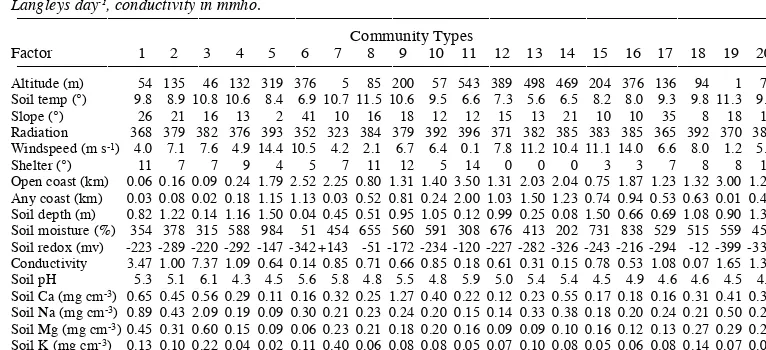
Table 4:Mean environmental factors for each of the Normal Clusters (Community Types 1-21). Radiation is in Langleys day-1, conductivity in mmho.
__________________________________________________________________________________________________________________________________
Community Types
Factor 1 2 3 4 5 6 7 8 9 10 11 12 13 14 15 16 17 18 19 20 21
__________________________________________________________________________________________________________________________________
Altitude (m) 54 135 46 132 319 376 5 85 200 57 543 389 498 469 204 376 136 94 1 70 79 Soil temp (°) 9.8 8.9 10.8 10.6 8.4 6.9 10.7 11.5 10.6 9.5 6.6 7.3 5.6 6.5 8.2 8.0 9.3 9.8 11.3 9.0 10.2 Slope (°) 26 21 16 13 2 41 10 16 18 12 12 15 13 21 10 10 35 8 18 10 5 Radiation 368 379 382 376 393 352 323 384 379 392 396 371 382 385 383 385 365 392 370 387 393 Windspeed (m s-1) 4.0 7.1 7.6 4.9 14.4 10.5 4.2 2.1 6.7 6.4 0.1 7.8 11.2 10.4 11.1 14.0 6.6 8.0 1.2 5.7 12.3
Shelter (°) 11 7 7 9 4 5 7 11 12 5 14 0 0 0 3 3 7 8 8 12 5
Open coast (km) 0.06 0.16 0.09 0.24 1.79 2.52 2.25 0.80 1.31 1.40 3.50 1.31 2.03 2.04 0.75 1.87 1.23 1.32 3.00 1.21 1.04 Any coast (km) 0.03 0.08 0.02 0.18 1.15 1.13 0.03 0.52 0.81 0.24 2.00 1.03 1.50 1.23 0.74 0.94 0.53 0.63 0.01 0.47 0.39 Soil depth (m) 0.82 1.22 0.14 1.16 1.50 0.04 0.45 0.51 0.95 1.05 0.12 0.99 0.25 0.08 1.50 0.66 0.69 1.08 0.90 1.30 1.50 Soil moisture (%) 354 378 315 588 984 51 454 655 560 591 308 676 413 202 731 838 529 515 559 456 785 Soil redox (mv) -223 -289 -220 -292 -147 -342 +143 -51 -172 -234 -120 -227 -282 -326 -243 -216 -294 -12 -399 -331 -294 Conductivity 3.47 1.00 7.37 1.09 0.64 0.14 0.85 0.71 0.66 0.85 0.18 0.61 0.31 0.15 0.78 0.53 1.08 0.07 1.65 1.37 0.90 Soil pH 5.3 5.1 6.1 4.3 4.5 5.6 5.8 4.8 5.5 4.8 5.9 5.0 5.4 5.4 4.5 4.9 4.6 4.6 4.5 4.2 4.2 Soil Ca (mg cm-3) 0.65 0.45 0.56 0.29 0.11 0.16 0.32 0.25 1.27 0.40 0.22 0.12 0.23 0.55 0.17 0.18 0.16 0.31 0.41 0.37 0.20
Soil Na (mg cm-3) 0.89 0.43 2.09 0.19 0.09 0.30 0.21 0.23 0.24 0.20 0.15 0.14 0.33 0.38 0.18 0.20 0.24 0.21 0.50 0.26 0.20
Soil Mg (mg cm-3) 0.45 0.31 0.60 0.15 0.09 0.06 0.23 0.21 0.18 0.20 0.16 0.09 0.09 0.10 0.16 0.12 0.13 0.27 0.29 0.28 0.24
Soil K (mg cm-3) 0.13 0.10 0.22 0.04 0.02 0.11 0.40 0.06 0.08 0.08 0.05 0.07 0.10 0.08 0.05 0.06 0.08 0.14 0.07 0.07 0.06
Growth index 2.35 1.54 2.50 0.57 0.35 0.45 1.52 0.84 2.15 1.00 1.29 0.64 1.05 1.68 0.58 0.70 0.57 0.99 1.24 0.87 0.59 Animal index 0.0 1.1 0.6 0.0 0.0 0.0 2.0 0.2 4.3 1.5 0.0 0.3 0.5 0.0 1.5 0.4 0.0 1.0 0.0 1.1 1.2
________________________________________________________________________________________________________________________________________________
Axis 1
The negative end of the axis (eigenvalue = 0.65) is characterised by the species groups R (e.g.,
Oreobolus, Centrolepis ciliata, Astelia), Q, ZA (e.g., scrub, fern, and epiphyte species), Y (Isolepis aucklandica, Coprosma perpusilla), and Z (Centrolepis pallida, Phyllachne). The positive end of the axis is characterised by the groups A (e.g.,
Puccinellia, Leptinella lanata, Crassula, Isolepis cernua), K (Cardamine depressa), M (Isolepis praetextata), S (Anisotome latifolia, Poa foliosa), E (Leptinella plumosa, Deschampsia chapmanii), D (Poa ramosissima), B (Hebe elliptica, Blechnum durum), H (Poa annua), C (Stilbocarpa, Pleurophyllum speciosum), I (Hydrocotyle), F (Isolepis habra), T (Poa litorosa, Bulbinella), and V (Carex appressa).
The vegetation gradient is related primarily to the complex of factors associated with proximity to the coast (Table 6). Shallowing of the peat/soil depth along the same gradient is the single most significant contributor to the 61% variation in stand positions accounted for using all sites. Upland rock ledge and outcrop vegetation have some affinities with maritime communities on shallow soils, which are reflected in their similar ordination positions. This relates to the higher mineral content of the rock ledge soils resulting in higher pH, and also the low grazing pressure allowing some palatable, typically maritime species to survive. The more coastal sites tend to be less steep, more shaded, and of course at lower altitude.
Using the 81 sites with the full complement of factors the multiple regression accounts for 73% of the variation (Table 6). Distance from the open coast is the most important contributor, with high soil Na levels and soil pH associated with more maritime, flushed, or biotically influenced sites. Wind speed tends to decline with proximity to the coast (or at low elevations).
By excluding proxy factors, the variation accounted for declines to 60% (Table 6). Presumably this is because the true causal factors are less accurately measured. Soil Na is strongly positively related to the gradient, and soil pH less strongly. Soil temperature increases and wind decreases along the fertility gradient.
Finally, when the growth index alone is considered the regression is significant but accounts for only 21% of the variation (Table 6). The altitude-related trends in soil temperature, and to some extent windiness, are incidental to this axis, since they are tied to the fertility gradient’s dependence on distance from the coast, and therefore indirectly to the inland higher-altitude sites at the negative end of Axis 1.
Figure 3:Typical examples of each of the Community Types (CT1-4). Altitude (in m) and distance from any coast (in km) are given for each sample site. A: Sample 13OG, CT1 - Maritime megaherb - tussock grassland (23 m, 0.02 km); dominated byPoafoliosa, Anisotome latifolia, Poa litorosa,andBulbinella rossii.B: Sample 19LB, CT2a - Upper maritimePoa-Bulbinellatall tussock grassland (27 m, 0.2 km); dominated byPoa litorosa, Bulbinella rossii,andPolystichum vestitum.C: Sample 10BG, CT2b - Upper maritimePoa-Bulbinella-megaherb tall tussock grassland (130 m, 0.25 km); dominated byAnisotome latifolia, Bulbinellarossii, Stilbocarpa polaris, Poa litorosa,
bog vegetation. On better drained and slightly less impoverished soils are dense, lowland heath (Dracophyllum) scrub and forest (CT20) and
Coprosma-fern-Myrsinescrub (CT18); at middle elevations are theChionochloatussock shrublands (CT17) and derivativePoameadows (CT15); and on the summits turf rush herbfields and fellfields (CT13, 14). Mesotrophic community types are in the middle band of the ordination, and receive some additional nutrients. Variously these come from some marine influence (CT19), flushing by enriched or oxygenated waters (CT10 - sedge swamp, CT5 - tarns and upland swamps), supplementation from guano (CT4), disturbance or grazing (CT5, 8, 9), or from being on free-draining, shallow mineral soils (CT6, 11, 12). At the most eutrophic end of the spectrum are maritime shrublands, tussock grasslands, and megaherbfields (CT1, 2), sea-elephant wallows (CT7), and bird colonies (CT4). At near-toxic cation levels are the littoral fringe cushions and turfs (CT3).
Axis 2
Species groups at the negative end of Axis 2 (eigenvalue = 0.48) are Q (dwarf forest associates), ZA (scrub and forest species), O (a lowland orchid associated with scrub margins), V (sedge swamp dominants), J (lowland fern), F (sedge swamp associates), U (the low to middle altitude
Chionochloa), R (lowland cushion bog species), and the various maritime species groups (A, B, M, D, E, S, K). The mid-axis segment includes T (Bulbinella, Poa litorosa), Y, P, I, and H (matrix turf species), X (low to middle altitude rush), C (megaherbs, shrub and grass), and W (widely distributed matrix species and upland
Marsippospermum). The positive end of the axis includes summit tundra groups L (Colobanthus hookeri, Epilobium pernitens), G (Grammitis poeppigiana, Poa aucklandica, Agrostis subulata), Z (Centrolepis pallida, Rostkovia, Pleurophyllum hookeri), and N (Cardamine subcarnosa). Groups W, Y, and T have species of wide amplitude.
The multiple regression on all sites accounts for 74% of the variation, and is overwhelmingly dominated by altitude (Table 6). Soil depth decreases with altitude (although this will be confounded with shallow soils near the littoral fringe). Higher altitude sites are less sheltered from the prevailing west wind. (The primary altitudinal gradient is negatively related to proximity to the coast.)
The full factor multiple regression accounts for 85% of variation. Altitude is still the major contributor, with minor contributions from soil Na (+ve), conductivity (-ve), soil Mg (-ve), and growth index (+ve).
The exclusion of proxy factors reduces the variation accounted for to 69%. The main contributors are soil Mg (-ve), soil temperature (-ve), Na (+ve), shelter (-ve), windspeed (+ve,
P< 0.1), soil pH (+ve), and growth index. However, the failure of growth index on its own to show any correlation with Axis 2, and the generally ambiguous contribution of the nutrient factors, is evidence that this second component of variation in the vegetation is principally altitude-controlled (via adiabatic air and ground cooling and by greater exposure to the wind). Soil depth declines towards rocky, eroding tops and other middle elevation outcrops that are at the top end of the ordination. And, whereas several nutrient factors decline towards the colder and more leaching environment of the summits, the important soil pH, soil Na, and the derivative growth index increase as a function of the freer draining mineral nature of the soils.
Thus, Axis 2 is simply an altitudinal (or thermal) gradient. The vegetation picture (Fig. 9) along this gradient conforms well with the environmental relations just described. At the base are sheltered dwarf forests and scrub (CT18, 19, 20), lowland bogs (CT21), swamps (CT10), and maritime or biotically induced communities (CT1, 2, 3, 4, 7). In mid-gradient are the middle elevation tussock grasslands (CT17) and induced meadows (CT4, 8, 9, 15); and at the top are the summit bogs (CT16), flushes or swamps (parts CT5, 12, 13, 16), rushlands (CT12, 13), fellfields (CT14), and rockfields (CT6, 11).
Axis 3
Axis 3 has an eigenvalue of 0.31. Species groups at the negative end are E (Rumex acetosella, Agrostis capillaris), H (Poa annua, Montia), K (Cardamine depressa), F (Pleurophyllum criniferum, Epilobium alsinoides), P (Juncus antarcticus), I (Hydrocotyle), X (Juncus scheuchzerioides), V (Carex appressa), and A (Colobanthus muscoides). The positive end of Axis 3 is characterised by groups D (Poa ramosissima), C (Stilbocarpa, Hebe benthamii), S (Poa foliosa, Anisotome latifolia), M (Isolepis praetextata), B (Hebe elliptica), N (Cardamine subcarnosa), and J (Hypolepis amaurorachis).
The multiple regression on all sites accounts for 29% of variation. There is a partly bimodal fertility gradient with high fertility at the negative end associated with mammals (animal index) and inland flushes, and again at the positive end associated with maritime influence (distance to open coast). Along this gradient there are increases in slope, soil depth and distance from any coast.
Table 5:Simple and partial correlation coefficients (r), and their probabilities (P), between pairs of environmental factors. Only significant correlations are listed.
__________________________________________________________________________________________________________________________________
Attribute Correlate Simple correlation Partial correlation
r P r P
__________________________________________________________________________________________________________________________________
Altitude Soil temperature -0.725 0.000 -0.500 0.000
Shelter -0.290 0.009
Distance to open coast 0.248 0.026
Distance to any coast 0.610 0.000 0.441 0.000
Conductivity -0.242 0.030
Soil Na -0.223 0.046
Soil Mg -0.535 0.000 -0.303 0.015
Growth index -0.236 0.034
Soil temperature Windspeed -0.376 0.001
Shelter 0.264 0.017
Distance to any coast -0.448 0.000
Conductivity 0.250 0.025
Soil Mg 0.347 0.002
Slope Radiation -0.689 0.000 -0.635 0.000
Windspeed -0.292 0.008
Shelter 0.356 0.001 0.328 0.008
Distance to open coast -0.291 0.008 -0.314 0.012
Distance to any coast -0.276 0.013
Soil depth -0.450 0.000 -0.256 0.042
Soil moisture -0.245 0.028
Soil pH 0.339 0.002
Growth index 0.336 0.002
Radiation Windspeed 0.356 0.001
Distance to open coast -0.278 0.026
Distance to any coast 0.277 0.012
Soil depth 0.346 0.001
Soil pH -0.302 0.006
Growth index -0.221 0.047
Windspeed Shelter -0.369 0.001
Distance to any coast 0.389 0.000
Soil moisture 0.330 0.003 0.263 0.036
Soil Mg -0.261 0.019
Shelter Distance to any coast -0.363 0.001
Distance to open coast Distance to any coast 0.605 0.000 0.567 0.000
Conductivity -0.338 0.002
Soil Ca -0.263 0.018
Soil Na -0.249 0.025
Soil Mg -0.360 0.001
Growth index -0.416 0.000
Distance to any coast Soil moisture 0.318 0.004
Conductivity -0.314 0.004
Soil pH -0.365 0.001
Soil Ca -0.291 0.008
Soil Na -0.457 0.000
Soil Mg -0.595 0.000
Soil K -0.307 0.005
Growth index -0.480 0.000
Soil depth Soil moisture 0.459 0.000 0.322 0.009
Soil pH -0.489 0.000
Soil Ca 0.283 0.023
Soil Na -0.354 0.001
Soil Mg 0.275 0.029
Soil K -0.378 0.001
Growth index -0.268 0.016
Animal index 0.217 0.051
Soil moisture Soil pH -0.485 0.000
Soil Ca -0.381 0.000
Soil Na -0.403 0.000
Soil Mg -0.442 0.000
Soil K -0.559 0.000 -0.252 0.044
Growth index -0.497 0.000
Soil Redox Soil pH 0.327 0.008
Soil Na -0.288 0.021
Soil Mg 0.275 0.028
Conductivity Soil pH -0.638 0.000
Soil Ca -0.392 0.001
Soil Na 0.610 0.000 0.805 0.000
Soil Mg 0.402 0.000 -0.518 0.000
Growth index 0.348 0.001 0.676 0.000
Soil pH Soil Ca 0.507 0.000 -0.256 0.041
Soil Na 0.427 0.000 0.523 0.000
Soil Mg 0.376 0.001 -0.499 0.000
Soil K 0.497 0.000
Growth index 0.686 0.000 0.691 0.000
Soil Ca Soil Na 0.269 0.031
Soil Mg 0.417 0.000 -0.408 0.001
Soil K 0.225 0.044
Growth index 0.821 0.000 0.761 0.000
Soil Na Soil Mg 0.704 0.000 0.671 0.000
Soil K 0.724 0.000 0.353 0.004
Growth index 0.360 0.001 -0.599 0.000
Soil Mg Soil K 0.594 0.000
Growth index 0.633 0.000 0.710 0.000
Soil K Growth index 0.335 0.002
Table 6:Statistics for multiple regression of environmental factors on vegetation ordination axes. The data are for those factor combinations with highest probability regressions (see below). Significance for 81 sites where the full complement of 19 environmental factors were measured is shown by asterisks (*). Regressions on all 134 sites but with only the 8 factors that were measured at all those sites (viz.altitude, slope, radiation, shelter, distance to open coast, distance to any coast, soil depth, and animal index), are indicated by +; • indicates significant regressions of factors at 81 sites excluding the proxy factors altitude, distance from open coast and distance from any coast (i.e., proxy factors where related direct factors were measured); # indicates significance of simple regression for 81 sites between vegetation scores and growth index. Probability levels are, respectivelyP< 0.05, 0.01 and 0.001 for 1-3 symbols of any type. Slope only is given whereP< 0.1.
__________________________________________________________________________________________________________________________________
Environmental Axis 1 Axis 2 Axis 3 Axis 4
factor Slope Contribution Slope Contribution Slope Contribution Slope Contribution
__________________________________________________________________________________________________________________________________
Altitude -0.001 5.1+ 0.005 91***+++ 0.001 42*++
Soil temperature 0.137 4.0• -0.135 8.6•• -0.095 5.1• 0.069
Slope -0.022 7.2+ 0.017 17++ -0.014 5.5*+
Radiation -0.012 5.9+
Shelter -0.015 5.8*+ 0.021 8.0*••
Distance to open coast -0.273 25**+++ -0.150 29**+++
Distance to any coast -0.291 19+++ 0.097 8.0+
Soil depth -0.802 38+++ -0.239 3.6++ 0.257 15++
Soil redox -0.001 5.0•
Conductivity -0.099 6.8* -0.102 5.1*
Soil pH 0.577 0.411 -1.003 24***•••
Soil Ca 0.658 7.7**•
Soil Na 1.110 5.1*• 0.753 7.5**•
Soil Mg -4.136 14*•••
Growth index 0.597 21### 0.355 0.601 5.2• -0.109 4.2#
Animal index -0.110 23*++• -0.049
Intercept 0.757 -0.437 6.658 3.598
__________________________________________________________________________________________________________________________________
significant soil pH (-ve) and distance to open coast (-ve) effect. The gradient also relates to shelter (+ve). Other significant soil factors are conductivity (-ve), soil redox potential (-ve), growth index (+ve), and soil Na (+ve). The significant animal index (-ve) is confirmed.
The multiple regression excluding proxy factors accounts for 52% of variation and has similar characteristics to the full factors regression. However, the significance of soil Na decreases and that of growth index and animal index increases. Soil temperature also decreases along the gradient, which perhaps reflects the environmental trends in the middle section of the ordination.
The soil factors which contribute to the growth index are contradictory here (i.e., Na and pH), and result in a non-significant simple regression with Axis 3.
Thus, the negative end of the Axis 3 gradient appears to be a miscellaneous assemblage of communities that are reduced in stature when compared with the zonal or optimal communities of the altitude sequence. These appressed turfs are on mammal-disturbed/grazed sites (CT7, 8), eroded peats (CT5), trampled tracks (CT9), flushed, waterlogged footslopes (CT10), and extreme maritime exposed rockfields (CT3). Flushing
appears to result in slightly reduced acidity, but this is not necessarily linked to other fertility factors. The fertility associated with the positive end of the axis results from maritime salt spray and seabird colonies on open coasts. There is a gradient from grazed sea elephant wallow banks (CT7), littoral-fringe cushion-turfs on rock (CT3), other short and/or discontinuous turf-mat grasslands, rushlands, and taller reed-like sedgelands (CT5, 8, 9, 10) on the one hand, to predominantly tall tussock grassland, megaherbfield (CT1, 2), scrub (CT19), and species-poor, stable seabird-induced swards (CT4). This may be understood in terms of a gradient from seral or rejuvenated (disclimax) communities to stable, more mature (climax or post climax) communities.
Axis 4
The species groups characteristic of the negative end of the axis (eigenvalue = 0.18) are C (Stilbocarpa), S (Anisotome latifolia), U (Chionochloa), and parts of A (Leptinella lanata), F (Pleurophyllum criniferum), E (Holcus), L (Taraxacum magellanicum), G (Ranunculus subscaposus), and V (Blechnum
Figure 7:Inverse (species) DCA ordination diagram for Axes 1 and 2. Axis 1 represents a fertility gradient with maritime species on the right, mesotrophic species in the centre, and bog species to the left. The vertical axis reflects an altitudinal gradient. Speciesí groups (guilds) are indicated by capital letters (see key).
amaurorachis), I (Hydrocotyle, Histiopteris, Pratia, Hypolepis millefolium), and parts of W(Stellaria decipiens), H (Stellaria media, Montia), and B (Hebe elliptica, Carex trifida).
The all sites multiple regression accounts for 14% of the variation. Altitude (+ve), slope (-ve), and animal index (+ve) are the significant contributors. The full factor sites multiple regression accounts for 41%, with soil Ca (+ve), slope (-ve), altitude (+ve), soil temperature (+ve), and growth index (-ve) the major contributors. With exclusion of proxy factors the multiple regression accounts for only 26% of variation and the overall regression is non-significant, with only soil Ca (+ve) a significant component. However, the simple growth index regression produces a significant negative relationship, although only 5% of the variation is accounted for.
Overall, Axis 4 appears to be a trend from tall
tussocks, sedges, rushes, megaherbs, and shrubs of relatively pristine and fertile condition (perhaps preserved in some instances by being associated with steep slopes) to appressed turfs and mats of grazed, disturbed, eroding, or rocky uplands accessible to feral mammals.
Autecology of the species
their imperfect contribution to the species associations and vegetation patterns. While the positions of species on the inverse ordination (Figs. 7, 8) indicate only their centroids in
multidimensional, environmental space, the mapping of species abundance at the individual stand loci on the normal ordination provides niche diagrams which offer a fuller appreciation of speciesí ecological limits (Figs. 11-15).
The species niche diagrams are juxtaposed to show the relationships of closely related or complementary species or growth forms in ordination space. Absolute environmental definition can be inferred from the factor overlays (Figs. 16, 17). In general the vertical axis of ordination 1 x 2 is treated as an altitudinal gradient and the horizontal axis as a fertility gradient from oligotrophic, acid soils on the left, through mesotrophic sites in the middle range, and eutrophic to maritime soils on the right. However, interpretation of the diagrams should bear in mind the following causes of distortion.
ï The ordination envelope is narrower at the top, presumably because the extreme summit environment tends to dampen the expression of other gradients that may be present.
ï The axes are only abstractions of real space, plant association gradients. Summit cushion bogs may tolerate the same degree of cold as fellfields, but because the latter form discontinuous vegetation the ordination analysis views them as more extreme than the mature, mesic herbfields below. Thus the uppermost sites within the envelope are not necessarily at the highest altitudes.
ï Likewise, the bottom of the diagram does not represent altitudes lower than those just above the Y-axis origin. It merely reflects the most sheltered, highly developed (forest) vegetation on the island, whereas the similarly elevated sites above the origin represent natural or induced open vegetation (mimicking tundra). Thus, species that fail to extend down to this origin are generally restricted to open spaces.
Figure 9:Normal (sites) DCA ordination diagram for Axes 1 and 2. Community Types are indicated by bold numbers.
• Some species, seriously depleted by past grazing history (or competition in part of their potential range), may not have reattained their full expression in the diagram. On the other hand, reduced competition will have allowed some herbaceous species to realise their physiological niche.
Fig. 11 displays the major shrub species. The order of diminishing tolerance of poor soils or occurrence on richer soils isDracophyllum scoparium(a calcifuge species),D. longifolium(a feature of riparian dwarf forests),Coprosma cuneata, Myrsine divaricata, Coprosma ciliata, Hebe benthamii, andH. elliptica. The mat-forming Coprosma perpusillaoccurs on the poorest soils alongside stuntedDracophyllum scoparium. All species may occur at or near sealevel, with adaptation to cold and exposure increasing in the orderH. elliptica, M. divaricata, D. longifolium, C.
ciliata, D. scoparium, C. cuneata, H. benthamii, andC. perpusilla.
Several cushion plants are typical of the saturated, oligotrophic, acid habitats.Centrolepis pallidais virtually confined to the uplands, while C. ciliatais the lowland representative of this genus (Fig. 11), usually occurring together with
Oreobolus pectinatusandAstelia subulata. Phyllachne clavigerais similarly restricted to impoverished soils, with a slight extension into summit fellfields and with greater tolerance of taller but open grassland vegetation. It differs from the other cushions mainly in straddling the complete altitudinal range.
is a summer-green, tall forb of mesotrophic lowland swamps and flushes. It is probably the least recovered species because (ecologically) it could not retreat from grazing animals into inaccessible refugia. Its habitat is island-like and therefore slow to be recolonised. The upland equivalent is the evergreenP. hookeri, although it frequents infertile as well as flushed, shallow soils. The widely tolerant and naturally widespreadP. speciosum
occurs at all elevations, from open maritime conditions to high altitude ledges on fertile to somewhat poor tussock grassland soils. The outlier ofP. criniferumto the left of the diagram is a good example of the occasional anomalies that relate to some undetected micro-environment or chance occupation of an otherwise inhospitable habitat.
Stilbocarpa polarisis another species of wide altitudinal range which also thrives on the richer to maritime sites.
Figure 10:Normal (sites) DCA ordination diagram for Axes 3 and 4. To the left on Axis 3 are sheep-grazed, sea elephant-disturbed, swamp, highly saline, littoral fringe and salt marsh sites. To the right is tall or dense maritime vegetation which may also be affected by seabirds. Axis 4 provides a different contrast between sheep-grazed and seabird nest sites above and maritime vegetation and swamps below.
The pair ofAnisotomespecies are clearly separated. The maritime to lowland, mesotrophicA. latifoliais seldom sympatric with the high altitude
A. antipoda, although this may change with their recovery. Interestingly, the latter species fills the lowland role on the Antipodes Islands in the absence ofA. latifolia(Godley, 1989). Hybrids are known among the species of bothAnisotomeand
antarcticais also widely spread in the open, inland communities which tend towards the oligotrophic.
Fig. 12 portrays the relationships of the grasses. The maritimePoa foliosaappears at the eutrophic end of the diagram where animal enrichment is also a factor.Poa litorosain its giant maritime phase extends almost as far. However, it is a much more versatile species and can cope with relatively oligotrophic sites and higher elevations as a bunch grass. The distribution ofP. foliosahas nevertheless been greatly reduced by grazing history, which may account for gaps at the base of the ordination diagram.Chionochloa antarcticais a low to middle altitude dominant (restricted at upper reaches by previous grazing), but especially tolerant of oligotrophic, acid bog soils. AlthoughP. litorosa
has replaced the palatableChionochloaover much of its former range, it is clearly vigorous (darker symbols) only in maritime or otherwise fertile flushes or sites influenced by sea animals. With the removal of sheep there is a gradual recovery of
Chionochloa, from resprouted bases or seed (Meurk, 1982), into the short tussock meadows (CT15) that have occupied the middle altitudes for most of this century.
The other tall grasses areHierochloespecies;H. fuscais typical of low-altitude, non-maritime though fertile sites such as swamps, whereasH. brunonisis an upland, mesotrophic, shorter-statured grass. The smaller matrix grasses fit among the taller
dominants.Poa ramosissimais very restricted at the eutrophic end of the spectrum being associated with seabird colonies.Poa breviglumis, Agrostis magellanica, andDeschampsia chapmaniiare low to middle elevation, mesotrophic species, whereasP. aucklandica, Agrostis subulata, andDeschampsia gracillimaare high altitude oligo-mesotrophs often associated with fellfields or rocks. Finally, three representative adventives (Agrostis capillaris, Festuca rubra, Poa annua), widely dispersed in the grazed meadows, are seen to require mesotrophic soils in this climate, and although the first two are known from high elevations on sheltered and sunny aspects they do not tolerate the exposed summit fellfields and bogs. Both theAgrostisandPoaare found in eutrophic sea elephant wallows.
Finally there are three forbs of saturated to semi-aquatic habitats (Fig. 12).Callitricheand
Montiaare sympatric in maritime and lowland eutrophic pools or on wet bare peat, especially in places disturbed and manured by seabirds and mammals.Neopaxiaoccurs at middle to higher elevations, also on flushed bare peat or among pebbles of talus and fellfield.
Rushes and sedges are presented in Fig. 13.
Marsippospermumis the dominant tall turf of
closed vegetation on high altitude, mesotrophic, sheltered sites andJuncus scheuchzerioides
occupies the mesotrophic, seral flushes, swamps, and eroded peats at middle to low elevations.
Rostkoviahas a role in the high altitude oligo-mesotrophic bogs and turf herbfields.Juncus antarcticushas a rather restricted distribution at middle altitudes in mesotrophic, short (grazed) turfy vegetation.LuzulaandUncinia hookeriare nearly ubiquitous open-space matrix species, the former spreading out a little further onto rock bluffs and ledges (upper extension of diagram), but neither tolerating extreme acidity.Uncinia aucklandicais confined to dwarf forests (lowland, oligotrophic part of spectrum).Carex appressadominates lowland, mesotrophic swamps, butC. trifidais a much less prevalent tussock of sheltered maritime sites. The four turfIsolepisspecies encompass the entire fertility spectrum of the island. Thus,Isolepis cernuaand the rarerI. praetextataare maritime species,I. habraoccupies mesotrophic flushes and disturbed ground to moderate elevation, andI. aucklandicais ubiquitous in open, meso-oligotrophic conditions.
The last group of larger physiognomic dominants comprises the ferns (Fig. 13).
Polystichum vestitumis most versatile in the lower to middle country, often defining gullies in both grasslands and dwarf forest, although avoiding extremes of soil fertility. The smaller, summer-green
P. cystostegiais restricted to the high altitude turf, rushlands, herbfields, and among rocks.Blechnum durumis confined to maritime tussock grasslands, banks, and ledges (sometimes under coastal bushes), with a distribution similar to the less common
Asplenium obtusatum.Blechnum“sp. 2” is most prevalent in mesotrophic sedge swamps and shrublands. The smallerB. penna-marinais found in only a few mossy swamps or grazed turfs. The summer-greenHypolepis millefoliumis rather localised in modified areas where grazing by sheep has been heavy, although it may be associated with scrub margins. These sites are mesotrophic but well drained.
Other pteridophytes include the filmy ferns (Fig. 13). These occur in mesotrophic to
oligotrophic conditions, althoughHymenophyllum minimumis generally epiphytic in dwarf forests.
common associate of lowland forest, scrub, and bogs on both mesotrophic and acid peats.
The orchidCorybas trilobusis fairly wide-spread from lowlands to uplands, sometimes in open meadows, but more commonly under the shelter and shade of tussock grassland or scrub. It appears to prefer mesotrophic conditions.
Small asterads includeDamnamenia, Leptinella, Abrotanella, Helichrysum, and
Lageniferaspecies (Fig. 14).Damnameniarosettes occur in meso-oligotrophic soils (rocks and fellfields to cushion bogs) at high elevations, but are confined to acid bogs near sealevel, where competition from taller vegetation is minimised. The plants may be small in adverse or exposed habitats and up to 15 cm diameter in more favourable conditions. TheLeptinellaspecies are found only in nutrient-rich sites,L. lanataforming mats along the littoral fringe and the tallerL. plumosain eutrophic, saturated, more sheltered, often animal influenced sites such as sea-elephant wallows.Abrotanella rosulatahas tiny rosettes that in aggregate form cushions in mesotrophic summit fellfields or on cliffs and ledges down to lower levels.Abrotanella spathulatais a small, mesotrophic, middle altitude meadow or intertussock rosette forb. In its lower reaches on grazed, mesotrophic turfs it overlaps with
Lagenifera petiolata. More widespread in
mesotrophic habitats of low to quite high elevation is the creepingHelichrysum bellidioides. It too requires high light levels in grazed meadows, swamps or rocky habitats where it is generally of high frequency.
The local members of the Caryophyllaceae are inconspicuous herbs and cushions (Fig. 14).
Cardamine subcarnosais an associate of upland herbfields and tall turf rushlands,C. corymbosais an often etiolated forb in middle elevation and maritime tussock grasslands, andC. depressais an infrequent diminutive rosette of exposed maritime turfs on cliff crests.Stellaria decipienshas a wider range, tolerating the shade of shrublands and dense tussocks as well as occurring frequently in open, grazed turfs or meadows. None of these species stray into the poorer, acid soils of the island.
Colobanthusis another genus with three species having clearly segregated niches. The high altitude fellfield locus is occupied byC. hookeri, a small cushion-former, the littoral fringe by the more robust cushion plantC. muscoides, and the maritime or open turfy, mesotrophic situation byC. apetalus. The successful adventiveCerastium fontanum
frequents the mesotrophic middle elevations in the grazed, short tussock meadows and other disturbed or anthropogenic sites. Apart from some of the
introduced grasses, this is the most successfully integrated alien plant.Geranium microphyllumis also mesotrophic, but with greater prominence at the upper end of its range. It is commonplace in the grazed, short tussock meadows at middle elevations and upland turf rushlands.
The rosaceous acaenas (Fig. 14) form clines and hybrid swarms, butAcaena minorsubsp.
minoris generally a distinct, matted forb of upland, open meadows, herbfields, and summit fellfields.
Acaena minorsubsp.antarcticais a more erect and robust, often bluish species typically associated with mesotrophic to maritime tussock grasslands and shrublands, tolerating a degree of shade. The possibly recently arrivedA. anserinifoliais more or less confined to the mesotrophic, sheep-grazed turfs and meadows. LikewiseAcaenacf. novae-zelandiaehas recently been discovered along sheltered harbour coasts.
Epilobium(Fig. 14) is, afterPoa, the largest genus in the island’s flora.Epilobium pernitensis a rather rare, upper tundra species which may grow in saturated, boggy ground. The subantarctic, endemic
E. confertifoliumis ubiquitous, and can tolerate both relatively poor and maritime soils.Epilobium pedunculareis also fairly versatile in middle to lower country, being able to grow both in the open meadows, mesotrophic swamps, and maritime grasslands and also in the shade of the more oligotrophic dwarf forests or shrublands.Epilobium alsinoidesis typically an erect forb of the lowland, tall sedge swamps, whereasE. brunnescensis a creeping plant of flushed and higher altitude turf herbfields, often grazed.Crassula moschatais a loose reddish cushion prominent in the littoral fringe. It is more etiolated and green in maritime situations, associated with tussocks.
Relating the species to the ordination of Axes 3 and 4 (Fig. 15), we note that Axis 3 represents proximity to sheltered water (cf. distance from any coast), high redox potential, and high direct animal influence (grazing or mechanical) to the left, and proximity to open water (cf. open coast) and high soil conductivity to the right. Axis 4 is a weak fertility gradient with generally higher values at the base related to maritime or flushed conditions (but not near-toxic levels of salt), whereas the upper axis (or positive end) is characterised by sites marginal to or previously affected by bird nesting (with perhaps only residually slightly elevated nutrient values). These environmental relationships are displayed in Fig. 17.