103
PREDICTIVE MODELLING AND VALIDATION FOR ESTIMATING
FODDER YIELD OF
GREWIA OPTIVA
S. E. H Rizvi**, Fehim Jeelani Wani*, Manish Kumar Sharma** and M Iqbal Jeelani**
*Division of Agricultural Statistics, SKUAST-K, Shalimar-190 025, India
**Division of Statistics and Computer Science, SKUAST-J, Chatha- 180 009, India *Correspondence; E-mail: [email protected]
Received: 20th December 2016 Revised: 2nd May 2017 Accepted: 16th May 2017
ABSTRACT Grewia optiva is one of the most important fodder trees of north-western and central Himalayas. It provides fodder during lean period of winter when there is scarcity of other fodders. For modelling, regression analysis was used to study the relationship between fodder yield (dependent variable) and other parameters. In total, more than 30 models (including linear and non-linear) were tried and on the basis of adjusted R2, the best five models were selected. These five models were validated for its adequacy through different criteria, namely, adjusted R2, bias, variance, root mean square error and coefficient of dispersion. On the basis of set criteria, the models were ranked. After applying the Wilcoxon signed rank test on fitting data set, one can arrive at the final ranks by considering ranks of both fitting (Rf) and validating (Rv) data sets. Finally, on the basis of all the criteria adopted in the present
investigation, out of the best five models, the regression model obtained as 𝑌̂ = 8.467 + 0.000004 (L2*S) ranked first, where 𝑌̂ = estimated fodder yield, L = average number of leaves per secondary branch (S), and hence recommended for fodder yield prediction of Grewia optiva.
Keywords: Grewia optiva, Modelling, Validation, Rank.
INTRODUCTION
Grewia optiva is one of the most important fodder trees of north-western and central Himalayas. It is a moderate sized tree, with a spreading crown, reaching height upto 12 m with clear bole of 3-4 m and girth 80 cm, when fully grown. Its leaves provide very nutritious fodder; the leaves and edible green twigs are palatable, nutritious and easily digestible. The leaves are rated as good fodder (Laurie, 1945). The green leaves constitute about 70 per cent of the total green weight of branches (Chandra and Sharma, 1977). The leaf fodder, when fed with straw or other inferior dry roughage
can profitably substitute concentrates. It is very heavily lopped for fodder which is the main use of the species (Sehgal and Chauhan, 1989). This system is practised in Jammu & Kashmir, Himachal Pradesh and Uttar Pradesh (Garhwal and Kumaon regions) Himalaya at the elevation of about 550 to 2,300m. As per literature, studies have been done on nutritional aspects as well as seed germination behaviour of
104
to feed their animals especially during lean period of winter when there is scarcity of other fodders. This information can be obtained through statistical modelling. Therefore, the present study on statistical modeling and validation for fodder yield estimation of Grewia optiva has been undertaken.
In India, equations for estimating biomass have been developed mainly for short rotation and timber species such as
Populus deltoides (Ajit et al. 2011; Rizvi et al. 2011), Eucalyptus (Ajit et al. 2000),
Dalbergia sissoo (Lodhiyal and Lodhiyal 2003; Bohre et al. 2012), Tectona grandis
(Buvaneswaran et al. 2006) and little attention has been paid for fodder and fuelwood species. Wani et al (2015) fitted different regression models for fodder yield estimation of Grewia optiva in Jammu Shiwaliks.
MATERIALS AND METHODS
The present study was conducted in Jammu region of Jammu and Kashmir State covering Shiwalik belt. Samba, Kathua and Udhampur districts were purposely selected. From each district two villages were randomly selected in order to select fodder trees from these villages as the ultimate unit for study purpose. The samples were collected from the population through Simple Random Sampling Without Replacement. Sample size was determined as per standard procedure (Cochran, 1977) and was calculated by using the formulae
2 2 2
d s t n
where s2 is sample variance, d is the permissible error.
Inorder to have a true representative sample from entire study area, a multistage sampling technique was adopted for the selection of sampling units in which districts were the first stage, villages within each district formed second stage units and
Grewia optiva trees in the selected villages were considered as the ultimate units.
The data for 60 trees selected randomly were collected for model development. A total number of 10 trees were randomly selected from each village so as to constitute a total sample size of 60 trees. Since it was not feasible to collect new data, the whole data set was divided into two sets by simple random sampling without replacement. The first data set (fitting data set) consisted of 30 observations and was used for fitting the models while the latter consisted of remaining 30 observations and was used for validation of fitted models.
For the purpose of developing a model for fodder yield estimation of Grewia optiva. The various parameters which are supposed to contribute towards fodder yield of Grewia optiva are as follows :
1. Height
2. Bole height
3. Diameter at breast height (dbh)
105
5. Secondary branches
6. Leaves per secondary branch
7. Canopy diameter
8. Age
For taking observations on above listed parameters the standard procedure as given in Forest Mensuration (Husch et al.
2003) has been followed.
Validation Technique:
Once a model which gives an adequate fit to the data has been found, the next step in the process is to use the model for prediction, or to learn about the mechanism, generated by the data. But before the model is to be used, its validity should be checked. A valid comparison of real data and model output in the validation stage requires an understanding of the nature of the problem plus the availability of statistical procedures which had been designed to fit the conditions of the problem. Ideally this can be done by using data not used earlier in either model formulation or calibrating. The most used methods for validation technique are half-splitting, cross-validation, jackknifing and bootstrapping. In the present investigation the technique of half-splitting has been used. In this method, the data are split in half by some means. Fitting (and possibly formulation) is carried out using the first half, and the results are evaluated using the second half. The roles of two halves are then reversed. Each evaluation provides an estimate of true error and the two estimates are averaged. Excess error is estimated by substracting off
apparent error obtained by fitting and evaluating on the entire data set.
For model validation, the estimates of Apparent error, True error and Excess error of model are critical. Apparent error (also called resubstitution error) is computed by applying the fitted equation to the data used in calibration of the model and will normally give an optimistic view of the quality of a model. True error is estimated by fitting the model to independent data (computed by applying the fitted equation to the data not used for calibration of the model). Apparent error underestimates the true error (“it is downwardly biased”). The difference between true error and apparent error is known as Excess error. The relationship can be formulated as :
True error = Apparent error + Excess error
Validation with independent set of data :
For the validation purpose, the data set parts has been divided into two through random procedure using SRSWOR with the help of random number table and the first data set (known as fitting data set) was used for the model building. The predictive ability of the different models were to be assessed on the basis of following evaluation criteria by using second data set (known as validating data set).
Average residual or prediction bias (B),
n r
B
i
106
Where, rirepresents the difference
between the observed and predicted fodder yield for ith tree in the validating data set. The variance of B is obtained by using formula:
1 )
( 1
2
n B r B
Var
n
i i
The root mean square error (RMSE) provides a composite measure (combining bias and precision) of the overall accuracy of prediction. The smaller these values the better the prediction.
B Var BRMSE 2
This Co-efficient of dispersion (CD) based on standard deviation, which measures the proportion variation in bias provides a composite measure of overall accuracy of prediction. The smaller the value, the better the prediction. Moreover it is unitless too. The CD is obtained by using following formula:
𝐶𝐷 = √𝑉𝑎𝑟(𝐵)
𝐵
All the procedures discussed so far belong to parametric tools. In addition some non-parametric technique could also be used so as to arrive at final decision criterion for selection of developed model. In this regard, Wilcoxon’s signed rank test (Wilcoxon, 1945) was used to test bias produced by each equation. This non-parametric test assumes that there is information in the magnitudes of the differences between paired observations, and rank them from
smallest to largest by absolute value. Add all the ranks associated with positive differences and then negative differences. Finally, the p-value associated with this statistic is found from an appropriate table. A rank was assigned to each equation based on each evaluation criteria (Cao et al., 1980). The smaller the rank value the better the performance of the model. These ranks of all criterion are then summed up to arrive at the final fit rank for each equation, which is the indicative of model’s performance with respect to all the criteria considered.
RESULTS AND DISCUSSION
Models
107
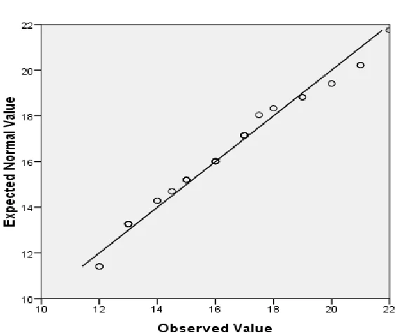
transformation and then fitting was made. The notation * in the different equation refers to multiplication term. In order to fulfil the assumption of the regression model, the normality of the dependent variable (fodder
yield) was checked through SPSS software with the help of Q-Q plot as shown below in Figure, and was found having normal distribution.
Table 4.1: Linear Models and other related characteristics
Models R2 Adj. R2 χ2
= -3.37 + 0.061L 0.885 (<0.001)
0.881 (<0.001)
1.48
= 5.95 + 0.00097(L)2 0.907 (<0.001)
0.904 (<0.001)
1.21
= 4.48 + 0.002(L*S) 0.894 (<0.001)
0.890 (<0.001)
1.35
= -7.13 + 0.311√L*S 0.891 (<0.001)
0.887 (<0.001)
1.39
= 8.467 + 0.000004(L2*S) 0.924 (<0.001)
0.921 (<0.001)
108
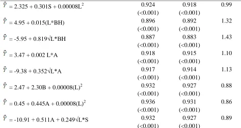
= 2.325 + 0.301S + 0.00008L2 0.924 (<0.001)
0.918 (<0.001)
0.99
= 4.95 + 0.015(L*BH) 0.896 (<0.001)
0.892 (<0.001)
1.32
= -5.95 + 0.819√L*BH 0.887 (<0.001)
0.883 (<0.001)
1.43
= 3.47 + 0.002 L*A 0.918 (<0.001)
0.915 (<0.001)
1.10
= -9.38 + 0.352√L*A 0.917 (<0.001)
0.914 (<0.001)
1.13
= 2.47 + 2.30B + 0.00008(L)2 0.932 (<0.001)
0.927 (<0.001)
0.88
= 0.45 + 0.445A + 0.00008(L)2 0.936 (<0.001)
0.931 (<0.001)
0.86
= -10.91 + 0.511A + 0.249√L*S 0.932 (<0.001)
0.927 (<0.001)
0.89
Figures given in parentheses indicate p-value, p-value < 0.01 indicates highly significant, L = Avg. number of leaves per secondary branch, S = number of secondary branches, BH = Bole height, A = age of tree
Table 4.2: Loglinear Models and other related characteristics
Models R2 Adj. R2 χ2
Ln = -3.943 + 1.165 Ln L 0.888 (<0.001)
0.884 (<0.001)
0.23
Ln = 3.393 + 0.717 Ln (L*S) 0.894 (<0.001)
0.890 (<0.001)
0.35
Ln = -3.750 + 0.453 Ln (L2*S) 0.912 (<0.001)
0.909 (<0.001)
0.29
Ln = -1.667 + 1.348 Ln √L*BH 0.890 (<0.001)
0.886 (<0.001)
0.41
Figures given in parentheses indicate p-value, p-value < 0.01 indicates highly significant
L = Avg. number of leaves per secondary branch, S = Number of secondary branches, BH = Bole height, A = Age of the tree
Out of the 17 models, the best five models were selected on the basis of
109
collinearity statistics i.e. tolerance and VIF (variance inflation factor) and error index of best five models are provided in Table 4.4. As the value of VIF was less than 10 for
each equation which indicates that there is low degree of collinearity present in the selected models.
Table 4.3: Best Five Selected Models
Equation Models R2 Adj. R2 χ2
1. = 8.467 + 0.000004(L2
*S) 0.924 (<0.001)
0.921 (<0.001)
0.98
2. = 2.325 + 0.301S + 0.00008L2
0.924 (<0.001)
0.918 (<0.001)
0.99
3. = 2.47 + 2.30BH + 0.00008(L)2 0.932
(<0.001)
0.927 (<0.001)
0.88
4. = 0.45 + 0.445A + 0.00008(L)2
0.936 (<0.001)
0.931 (<0.001)
0.86
5. = -10.91 + 0.511A + 0.249√L*S
0.932 (<0.001)
0.927 (<0.001)
0.89
Figures given in parentheses indicate p-value, p-value < 0.01 indicates highly significant
L = Avg. number of leaves per secondary branch, S = Number of secondary branches, BH = Bole height, A = Age of the tree
Table 4.4 : Equations with other related characteristics
Equations e* e** Collinearity statistics Error index
Tolerance VIF
1 0.061 0.042 1 1 10.20
2 0.063 0.031 0.414 2.418 9.98 3 0.052 0.035 0.487 2.055 9.47 4 0.054 0.034 0.539 1.855 8.99 5 0.055 0.035 0.510 1.963 9.15
From the perusal of the literature, it was observed that in general, for comparing models the following error index has been used given by
∑ wi | ei | / n
Where, wi is the quantity related to the
110
obtaining the critical errors of models, Ek and Monserud (1979) suggested lower (e*) and upper (e**) bounds of anticipated error due to model.
Table 4.3 gives five fitted models. This table also depicts the adj. R2 and calculated chi-square values. Table 4.4 gives the other related characteristics like e*, e**, collinearity statistics and error index of the fiited models. From Table 4.3 it may be inferred that the value of adj. R2 for the model 4 is maximum followed by model 3 and model 5, respectively, whereas the error index for the model 5 is less than the error index of the model 3 having same value of adj. R2. This brought into light that the value of adj. R2 is not sufficient for recommendation of the model. The values of χ2
and error index are the other characteristics which decide the recommendation of the model. The collinearity statistics given in Table 4.4 shows there is no multicollinearity present in
the models. The value of tolerance for the first model 1 is maximum followed by model 4, whereas the VIF is maximum for model 2 and minimum for model 1. The 1st and 2nd column of Table 4.4 gives the lower and upper bounds of error index. Shortening of the intervals is a sufficient proof of increased accuracy, on the basis of this model 3 as best followed by model 1. On the basis of the criterion of adj. R2 and error index the model at serial number 4 as best followed by model at serial number 5.
Model Validation
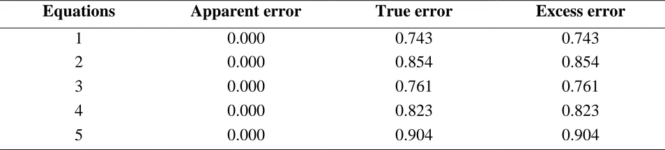
In order to assess the predictive ability of the different equations, the models were validated by using independent data set (known as validating data set). For this purpose, the equations obtained from the fitting data set were applied to the validating data set . The apparent error, true error and excess error were calculated for each equations and is given in Table 4.5.
Table 4.5: Values of errors of equations
Equations Apparent error True error Excess error
1 0.000 0.743 0.743
2 0.000 0.854 0.854
3 0.000 0.761 0.761
4 0.000 0.823 0.823
5 0.000 0.904 0.904
In general, apparent error comes to zero for regression models, which means that the
111
better the predictive ability of the equation. From Table 4.5 which gives the values of errors of the equations, it can be concluded that Equations 1, 2, 3 and 4 has given reasonable values of excess error, whereas Equation 5 has given the highest value of excess error, which means that the predictive ability of Equation 5 is poorer than other equations in case of excess error
criterion. Whereas the predictive ability of Equation 1 may be judged as best than other equations. The predictive ability of the different models were assessed on the basis of different criteria, namely, adj. R2, bias, variance, root mean square error and coefficient of dispersion. The validation statistics for equations with independent data set is given in Table 4.6.
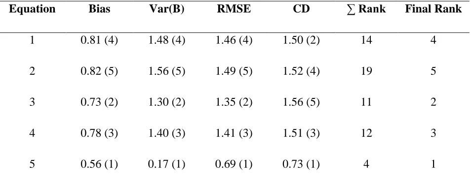
Table 4.6: Validation statistics for equations with independent data set
Equation Bias Var(B) RMSE CD ∑ Rank Final Rank
1 0.81 (4) 1.48 (4) 1.46 (4) 1.50 (2) 14 4
2 0.82 (5) 1.56 (5) 1.49 (5) 1.52 (4) 19 5
3 0.73 (2) 1.30 (2) 1.35 (2) 1.56 (5) 11 2
4 0.78 (3) 1.40 (3) 1.41 (3) 1.51 (3) 12 3
5 0.56 (1) 0.17 (1) 0.69 (1) 0.73 (1) 4 1
Note: numbers in brackets ( ) refers to the ranks from smallest to largest value
It can be observed from Table 4.6 that Equation 5 has the lowest value of bias (0.56) whereas Equation 2 has highest value of bias (0.82). In case of variance, Equation 2 has highest value (1.56) whereas Equation 5 has lowest value (0.17). The combined effect of bias and variance is expressed as RMSE. With regard to RMSE, Equation 5 has the least value (0.69) whereas Equation 2 has the highest value (1.49). Coefficient of dispersion has also been calculated to
112
The non-parametric test (Wilcoxon’s signed rank test) was used to test the bias produced by each equation. The Wilcoxon’s
signed rank test and combined result of the criterion ranks is given in Table 4.7.
Table 4.7: Wilcoxon’s signed rank test and combined result of the criterion ranks
Equation Z Asymptotic
significance
Rf Rv ∑ Rank Final
Rank
1 -1.351 0.177 1 4 5 1
2 -1.049 0.294 2 5 7 3
3 -0.162 0.871 4 2 6 2
4 -0.184 0.854 3 3 6 2
5 -0.119 0.905 5 1 6 2
Rf – Rank of fitting set Rv – Rank of validating set
On the basis of asymptotic significance, the ranks to the fitted equations were given. The equation with lower value has been given the first rank, whereas the equation with higher value has been given the last rank. The ranks of the validating set as obtained in Table 4.6 were put together with the ranks
for fitting data set as depicted in Table 4.7. By combining the ranks of both the fitting as well as validating data sets, we get the summation of ranks and final ranking was made on this sum of ranks. Finally, on this basis of selection, the equation 1 gets the first rank. Hence the following model
= 8.467 + 0.000004 (L2*S) (R2 = 0.924)
113
Thus, the above model can be used for predicting fodder yield of Grewia optiva
giving the number of leaves per secondary branch and number of secondary branch. From the economic point of view, we can easily estimate the fodder yield of each tree using this model and can disseminate this information to farmers that how much revenue they will get from each tree by selling fodder during winter, when there is scarcity of other fodder trees.
SUMMARY AND CONCLUSION
For model development, the data recorded on green fodder yield and yield attributing characters for all the 60 randomly selected trees were utilized. In all, more than
30 models (including linear and non-linear) were tried on the fitting data set. Out of total models tried, the best five models were selected on the basis of adj. R2 value. Goodness of fit of the selected models was also tested by applying chi-square test. The chi-square test results came out to be insignificant and hence we accepted the null hypothesis under test, indicating thereby that the models under study qualified for goodness of fit test and could be used for prediction purposes after validation. The critical error, error index and collinearity statistics were calculated for each model. The collinearity statistics include tolerance and Variance Inflation Factor (VIF), and it was found that multicollinearity was not present in the selected models. The equations of best five models obtained are listed below.
R2 adj. R2
Equation 1 𝑌̂ = 8.467 + 0.000004(L2*S) 0.924 0.921 Equation 2 𝑌̂ = 2.325 + 0.301 S + 0.00008 L2 0.924 0.918 Equation 3 𝑌̂ = 2.47 + 2.30 BH + 0.00008 L2 0.932 0.927 Equation 4 𝑌̂ = 0.45 + 0.445 A + 0.00008 L2 0.936 0.931 Equation 5 𝑌̂ = -10.91 + 0.511 A + 0.249√L*S 0.932 0.927
For model validation, the estimates of Apparent error, True error and Excess error are critical. It was found that Equation 1 has given the lowest value of excess error (0.743) which means that the predictive ability of Equation 1 is better than other equations. The model adequacy was ranked on the basis of different criteria, namely, adj.
114
combined effect of bias and variance is expressed as RMSE and based on this criteria here Equation 5 has the least value(0.69) whereas Equation 2 gave the highest value (1.49). As regards to CD value, Equation 5 has the least value (0.73) and the highest value (1.56) was obtained for Equation 3. After considering all the ranks, Equation 5 was ranked as first followed by 3, 4, 1 and 2 ,on the basis of above stated criteria.
Finally, the non-parametric test (Wilcoxon signed rank test) was also used to test bias produced by each equation. This non-parametric test assumes that there is information in the magnitudes of the differences between paired observations. The asymptotic significance of Wilcoxon’s signed rank test for validating data set for all equations showed that the null hypothesis of test, i.e. the difference between sum of the positive and negative rank is zero is accepted. By considering ranks of both fitting (Rf) and validating (Rv) data sets, one
can arrive at the final ranks. The overall rank of Equation 1 was lowest indicating thereby that this equation would perform better for predicting green fodder yield per tree of Grewia optiva specie. Therefore, it can be concluded that Equation 1 should be preferred over other equations considered for present study.
REFERENCE
Ajit Das DK, Chaturvedi OP, Jabeen N, Dhyani SK (2011). Predictive models for dry weight estimation of above and
below ground biomass components of
Populus deltoides in India:
development and comparative diagnosis. Biomass and Bioenerg
35:1145–1152.
Ajit VK, Gupta KR, Kumar RV, Datta A (2000). Modelling for timber volume of young Eucalyptus tereticornis
plantations. Indian J of For, 23: 233– 237.
Bohre, P., Chaubey, P and Singhal, K. (2012). Biomass accumulation and carbon sequestration in Dalbergia sissoo Roxb. International Journal of
Bio-Science and Bio-Technology
4(3):29–44.
Buvaneswaran, C., George, M., Perez, D. and Kanninen, M. (2006). Biomass of teak plantations in Tamil Nadu, India and Costa Rica compared. J Trop For Sci18(3):195–197.
Cao, Q. V., Burkhat, H. E. and Max, T. A. (1980). Evaluation of two methods for cubic volume prediction for Loblolly pine to any merchantable limit.
Forestry Science, 26: 71-80.
Chandra, J.P. and Sharma, R.K. (1977). Note on nursery technique of beul
(Grewia oppositifolia). Indian
Forester, 103(10): 684-5.
Cochran, W. G. (1977). Sampling techniques, New York: John Wiley & Sons.
115
Husch, B., Beers, T. W. and Kershaw, J. A. (2003). Forest Mensuration. John Wiley & Sons, INC.
Laurie, M. V. (1945). Fodder trees in india. FRI, Dehradun, 17-82.
Lodhiyal N, Lodhiyal, LS (2003). Biomass and net primary productivity of Bhabar Shisham forests in central Himalaya, India. For Ecol Manag176:217–235.
Negi, S. S. (1986). Foliage from forest trees: a potential feed resource. In: Agro forestry Systems: a new challenge. ISTS, Solan, 111-120.
Rizvi, H., Dhyani, K., Yadav S and Ramesh S (2011). Biomass production and carbon stock of poplar agroforestry systems in Yamunanagar and Saharanpur districts of North western.
India. Curr Sci, 100: 736–742.
Sehgal, R. N. and Chauhan, V. (1989).
Grewia optiva an ideal agroforestry tree of western Himalaya. Farm
Forestry News 5. Winrock
International, USA.
Vanclay, J. K. (1994). Modelling forest growth: Application to mixed tropical
forests. CAB international,
Wallingford.
Wani, F. J.., Rizvi, S. E. H and Sharma, M. K. (2015). Statistical Modelling for fodder yield estimation of Grewia
optiva in Jammu Shiwaliks.
International Journal of Agricultural and Statistical Sciences. 11(1): 139-142.