Explicit Multistep Block Method for Solving Neutral Delay
Differential Equation
Nur Inshirah Naqiah Ismail1, Zanariah Abdul Majid∗1,2, and Norazak Senu1,2 1Institute for Mathematical Research, Universiti Putra Malaysia, 43400 UPM Serdang,
Selangor, Malaysia.
2Department of Mathematics, Faculty of Science, Universiti Putra Malaysia, 43400
UPM Serdang, Selangor, Malaysia.
∗Corresponding author:am [email protected]
The aim of this paper is to solve the initial-value problem for single first order neutral delay differential equation (NDDE) of constant delay type by applying explicit method. In order to find the approximate solution of the problem, a two-point explicit multistep block method has been derived by implementing Taylor series interpolation polynomial. The method obtained will compute numerical solution to solve NDDE problem at two points simultaneously using constant stepsize. The delay solutions of the unknown function will be interpolated using previous values and the derivative of the delay terms will be obtained by applying divided difference formula. The main implementation idea of the method is based on the multistep method formula. The order and consistency of the method will be discussed in methodology section. Numerical results presented have shown that the proposed block method is more accurate than the implicit multistep block method and is suitable and efficient for solving first order NDDE of constant delay type. Keywords: Constant delay, Initial-value problem, Explicit Multistep Block Method, Neutral Delay Differential Equation
I.
Introduction
Nowadays, dynamical system involving time delays have played a very important role in solving real life phenomena with their applications in biological and physiological processes. For instance, the delay term can be presented as a transport delay which can be described as a signal to travel to the controlled object as quoted by (Kuang, 1993). In mathematics, Delay Differential Equations (DDE) are assumed to have occured in many different fields of science, mathematics and technology. DDE are defined as an equation which the derivatives of a function at present time is dependable on the function at previous time. DDE is also known as different names by different researchers such as a time-delay systems, hereditary systems, equations with deviating argument or differential difference
of an implicit and explicit NDDE may have discontinuous derivatives (Baker and Paul, 2006). The one-leg θ methods have been discussed by (Wang and Li, 2007) for the numerical solution of NDDE with pantograph delay. The method is then being compared with variational iteration method (VIM) which has been applied by (Chen and Wang, 2010) for the numerical solution of NDDE. A two-point variable order variable stepsize block method for the numerical solution of DDE has been described by (Ishak et al., 2008). A homotopy pertubation method (HPM) has been applied to solve NDDE and the effectiveness of the method has also been revealed by (Biazar and Ghanbari, 2012). Both VIM and HPM are included in the class of analytical method where the results obtained have known to approach the exact solution even with a few iterations. The development of block method for NDDE problems has then being described by (Ishak et al., 2014) where they have derived an implicit two-point block method in variable stepsize technique. Later, an implicit three-point one-block method for solving first order NDDE using variable stepsize has been developed by (Ishak and Ramli, 2015). A two-point block method to solve NDDE of pantograph type which is also an implicit method has been used by (Seong and Majid, 2015) to solve NDDE problems. Most of the authors have been proposing implicit block multistep method or one-step block method in the predictor-corrector scheme and none of them seemed to applied an explicit multistep block method for solving NDDE. Some of the authors have also proposed analytical methods for the solution of NDDE problems. NDDE is a differential equation which consists of different types of delay such as constant, pantograph, state-dependent and even a discontinuity of delay case. As a number of authors have been solving these cases using different approaches, this has motivate our research to focus more on solving and handling constant NDDE using explicit multistep block method. As known by many researchers, it is
sometimes difficult and impossible to obtain analytical solutions for DDE and thus the best approach is to use numerical methods in order to approximate the solutions as accurate as possible. The motivations of proposing an explicit method are because the method itself have owned many advantages that are unseen by many researchers especially in treating differential equations with delays.The advantages in using explicit method is it has reduced the computational cost, produced faster results, consumed lesser time and has simple computational calculation than any implicit method. In this study, a first-order NDDE is considered as follows:
y0(x) =f(x, y(x), y(x−τi), y0(x−σi))
y(x) =φ(x), x≤a
y0(x) =φ0(x), x≤a
(1)
where τ(x, y(x)) and σ(x, y(x)) are the delays while y(x−τ(x, y(x))) and y0(x−σ(x, y(x))) are the expressions of delay solutions. Any divided difference formulas will be applied in order to solve the delay derivatives. A two-point explicit block method which is based on multistep method formula will approximate the solutions at two point simultaneously using constant stepsize.
II.
Methodology
In this section, the development of two-point block method will be explained briefly. A block method to solve NDDE is adapted from (Majid and Suleiman, 2011). First order NDDE as mentioned in (1) is considered. In order to compute the two approximation values of yn+1 and yn+2 simultaneously, the
interval [a, b] is divided into a series of blocks with constant stepsize given by, a =
x0, x1, ..., xn−1, xn, xn+1, ..., xN = b and each
Figure 1: Two-Point Block
Suppose the kth block contains xn−2, xn−1
and xn, where xn−2 will be set as the starting
point and xn is the last point in the kth block
with stepsize h. The evaluation solution at the last point in kth block will be used as the
initial values for (k+1)thblock. The next block will be calculated using the same procedure until reaching the end point of the interval. Let yn(xn) be the approximated solution and
y(xn) is the exact solution of y at point xn.
The approximation values ofyn+1andyn+2are
computed simultaneously.
A. Formulation of the Method
Definition 1. Linear difference operator L associated with
k
X
j=0
αjyn+j =h k
X
j=0
βjfn+j (2)
is given by
L[y(x) :h] =
k
X
j=0
[αjy(x+jh)
−hβjy0(x+jh)
(3)
expanding y(x+jh) and y0(x+jh) as Taylor series about x and collecting terms will give
L[y(x) :h] =C0y(x) +C1y(1)(x) +...
+Cphpy(p)(x).
(4)
The current task is to evaluateyn(xn+1) and
yn(xn+2) as well as their corresponding delay
and delay derivative solutions. The expression
f(x, y(x), y(x−τi), y0(x−σi)) will be denoted as
fn. The approximation ofy(xn+1) andy(xn+2)
are obtained by Taylor series polynomial in the
forms:
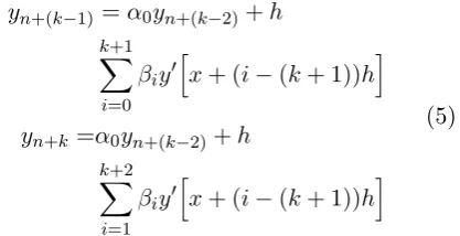
yn+(k−1) =α0yn+(k−2)+h k+1
X
i=0
βiy0
h
x+ (i−(k+ 1))hi
yn+k=α0yn+(k−2)+h k+2
X
i=1
βiy0
h
x+ (i−(k+ 1))hi
(5)
where the value of k is 2. Letting α0 = +1,
expanding individual terms in (5) using Taylor series expansion, substituting the expansion back in (5) and collecting the terms will give:
h
y(x) + 4hy0(x) + 8h2y00(x) +32 3 h
3y000(x)
+ 32 3 h
4y0000(x)i=hy(x) + 3hy0(x)+
9 2h
2y00
(x) +9 2h
3y000
(x) +27 8 h
4y0000
(x)
i
+hβ0 h
y0(x)
i
+hβ1 h
y0(x) +hy00(x)+
1 2h
2y000(x) + 1
6h
3y0000(x)i+hβ
2 h
y0(x)
+ 2hy00(x) + 2h2y000(x) +4 3h
3y0000
(x)
i
+
hβ3 h
y0(x) + 3hy00(x) +9 2h
2y000
(x)
+ 9 2h
3y0000(x)i
(6)
and
h
y(xn+1) + 4hy0(xn+1) + 8h2y00(xn+1)
+32 3 h
3y000(x
n+1) +
32 3 h
4y0000(x
n+1) i
=
h
y(xn+1) + 2hy0(xn+1) + 2h2y00(xn+1)
+4 3h
3y000
(xn+1) +
2 3h
4y0000
(xn+1) i
+
hβ1 h
y0(xn+1) i
+hβ2 h
y0(xn+1)+
hy00(xn+1) +
1 2h
2y000(x
n+1)+
1 6h
3y0000
(xn+1) i
+hβ3 h
y0(xn+1)
+ 2hy00(xn+1) + 2h2y000(xn+1)+
4 3h
3y0000(x
n+1) i
+hβ4 h
y0(xn+1)
+ 3hy00(xn+1) +
9 2h
2y000(x
n+1)
+9 2h
3y0000
(xn+1) i
.
Collecting terms from (6) and (7) and equating coefficients of ymx
n yields to the following
block:
yn+1 =yn+
h
24
h
55fn−59fn−1+ 37fn−2 −9fn−3
i
yn+2 =yn+
h
3
h
8fn+1−5fn+ 4fn−1 −fn−2
i
.
(8)
The method obtained above is a two-point explicit multistep block method (2PEBM) which will be applied to solve neutral class of DDE. The order and convergence of the block method will be discussed in section 2.2 and 2.3 respectively. The implementation on how the delay terms will be treated will be explained in section 2.4.
B. Order of Method
Definition 2. A linear multistep method (2)is said to be of order pif,C0 =C1=...=Cp = 0 and Cp+1 6= 0 is called as error constant.
Cp=
k
X
j=0 hjpαj
p! −
jp−1βj
(p−1)!
i
(9)
where p= 0,1,2, ...
The order and error constant of 2PEBM can be obtain from:
C0 =
k
X
j=0
αj =
0 0
C1 =
k
X
j=0
(jαj−βj) =
0 0
C2 =
k X j=0 (j 2α j
2! −jβj) =
0 0
C3 =
k X j=0 (j 3α j 3! −
j2βj
2! ) =
0 0
C4 =
k X j=0 (j 4α j 4! −
j3βj
3! ) =
0 0
C5 =
k X j=0 (j 5α j 5! −
j4βj
4! ) =
251/720 29/90
.
This implies that the block method has order 4 (2PEBM4) with error constant C5 =
(251720,2990)T.
C. Convergence of Method
Based on (Lambert, 1973), linear multistep method (2) is said to be converge if and only if the method is consistent and zero-stable. Thus two analyses have been formulated to prove the consistency and zero-stability of the explicit method respectively.
Definition 3. A linear multistep method (2)is said to be consistent if it has order p >1 and the method is consistent if and only if
k
X
j=0
αj = 0 and
k
X
j=0
jαj = k
X
j=0
βj (10)
Explicit multistep block method (8) will be rewritten in the form shown below:
1 0 0 1
yn+1
yn+2 = 0 1 0 1
yn−1
yn
+h
−249 3724
0 −1 3
fn−3
fn−2 +h −59 24 55 24 4 3 − 5 3
fn−1
fn +h 0 0 8 3 0
fn+1
fn+2
(11)
where (11) is equivalent to:
A2YN+2=A1YN+1+h 2 X
j=0
Following condition in (10):
k
X
j=0
αj =
5 X
j=0
αj =α0+α1+α2
+α3+α4+α5
=
0 0
followed by:
k
X
j=0
jαj = k
X
j=0
βj
where
k
X
j=0
jαj = 5 X
j=0
jαj = 0·α0+ 1·α1+ 2·α2
+ 3·α3+ 4·α4+ 5·α5
=
1 2
and
k
X
j=0
βj = 5 X
j=0
βj =β0+β1+β2
+β3+β4+β5
=
1 2
Hence, it is shown that
k
X
j=0
αj = 0 and
k
X
j=0
jαj = k
X
j=0
βj =
1 2
. As 2PEBM4 in (8)
has order 4 = p ≥ 1, thus the conditions on consistency stated in Definition 3 have been proved and 2PEBM4 is concluded to be consistent.
According to (Lambert, 1973) on zero-stability interpretation,
Definition 4. The linear multistep method (2)
is said to be zero-stable if no root of the first characteristic polynomial:
ρ(ξ) =
k
X
j=0
αjξj = 0 (13)
has modulus greater than one.
In such a way,
ρ(ξ) =
5 X
0
αjξj =α0ξ0+α1ξ1+α2ξ2
+α3ξs3+α4ξ4+α5ξ5
=
ξ3(−1 +ξ)
ξ3(−1 +ξ2)
From the above interpretation, a conclusion on the roots of (13) are achieved as there will be no root has modulus greater than one. Following (Lambert, 1973), 2PEBM4 is converge as it has satisfied both consistency and zero-stability conditions.
D. Implementation of the Method
By considering the first order constant NDDE as denoted in (1), the 2PEBM4 in (8) will be used to obtain the approximate solutions of the problems. Since (8) needs to have four previous values to complete the calculation with only one given information which is the initial value, therefore three starting values will be computed using one-step method. Runge-Kutta order 4 (RK4) has been chosen to find the initial solutions as it has the same order with 2PEBM4. In handling the delay terms for neutral class of DDE, two different functions of delay need to be considered which are the delay that involved its derivative of unknown previous function and the one that does not involve the estimation of the derivative function. The location of the delay must first be determined to obtain the solution of y(x − τi) and y0(x −
σi). For constant type of NDDE problems,
in (1). The formula for backward difference is shown below:
y0(x−σi) =
y(x−τi)−(y(x−τi)−h)
h .
As the value of the delay functions are sufficient enough, the forward difference formula shown below can be applied:
y0(x−σi) =
(y(x−τi) +h)−y(x−τi)
h .
If the delay itself, x−τi < a, then the initial
function given in (1) needs to be applied to solve the delay terms. But, if x −τi ≥ a,
then the delay terms need to be solved by using Lagrange interpolation polynomial in the form:
P(x) =Ln,0(x)f(x0) +. . .+Ln,n(x)f(xn)
=
n
X
k=0
f(xk)Ln,k(x)
where
Ln,k(x) = n
Y
i=0 i6=k
(x−xi)
(xk−xi)
k= 0,1, . . . , n.
As mentioned above, 2PEBM is implemented based on the multistep method formula and the block method produced approximations for
yn+1 and yn+2 simultaneously. The algorithm
of the proposed block method is developed in C language by using constant step size.
Algorithm
Step 1: Set values for a, b, N, h and the given initial value.
Step 2: Use RK4 for approximating the starting values.
Step 3: If x−τi < a, compute the delay
terms by using initial function given in (2).
Ifx−τi≥a, then the delay terms
need to be solved by using Lagrange interpolation polynomial:
P(x) =Ln,0(x)f(x0) +. . .+Ln,n(x)f(xn)
=
n
X
k=0
f(xk)Ln,k(x).
Step 4: Fori= 1,3, . . .
y0(x−τi) is obtained by applying
backward difference formula.
The approximate valueyn+i is evaluated
by using:
yn+i =yn+ 24h
h
55fn−59fn−1
+37fn−2−9fn−3 i
.
Step 5: Fori= 2,4, . . .
y0(x−τi) is obtained by applying
forward difference formula.
yn+i =yn+ h3
h
8fn+1−5fn
+4fn−1−fn−2 i
.
Step 6: If the functions of delay terms are adequate to be included in
iterations, then forward difference formula can be applied.
Step 7: End.
III.
Results and Discussion
(Ishak and Ramli, 2015):
Example 1.
y0(x) =y(x) +y(x−1)−1
4y
0(x−1), x∈[0,1]
y(x) =−x, x≤0
y(x) =−1
4 +x+ 1
4exp(x), x∈[0,1]
Example 2.
y0(x) =y(x) +y(x−1)−2y0(x−1), x∈[0,1]
y(x) =−x, x≤0
y(x) =−2 +x+ 2 exp(x), x∈[0,1]
Example 3.
y0(x) =y(x) +y0(x−1), x∈[0,1]
y(x) = 1, x≤0
y(x) =exp(x), x∈[0,1]
Example 4.
y0(x) =y(x) +y(x−1)−1
4y
0(x−1) +sin(x),
x∈[0,1]
y(x) = 1, x≤0
y(x) =−1
4 +x+ 3
4exp(x)− 1
2cos(x)− 1
2sin(x),
x∈[0,1]
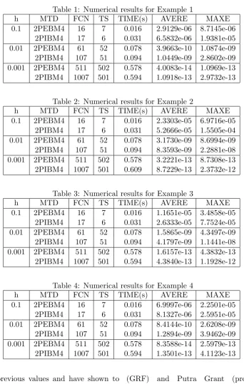
Numerical results for Example 1 - 4 are displayed in Table 1 - 4. From the numerical results obtained, it is observed that the proposed method, 2PEBM4 is more accurate and efficient than 2PIBM4. An implicit method has been said to have more accurate results than the explicit method as the computation of the implicit method involved both approximation of predictor and corrector scheme. Theoretically, a predictor-corrector form method will produce better results in terms of accuracy but in neutral delay case, an explicit method has out performed the implicit method. As shown in numerical results below, 2PEBM4 is proved to have better average and maximum errors than 2PIBM4. Based on previous literature review, it has been
observed that no explicit multistep method has been applied in solving NDDE. The delay behavior is known to be slow and sensitive to be handled using high performance method while an explicit method is said to be less effective than the implicit method in solving differential equations. Thus, this concludes that they are both suitable to be pair as they have already shared the similarity. The function evaluation has also been chosen as one of the parameter because the explicit method apparently has less function evaluation than an implicit method and also to highlight an extra advantage for applying the explicit method. Other benefit of using 2PEBM4 is the method managed to decrease the time taken in computing all the approximate solutions and its total function call compared to 2PIBM4. Besides, the explicit method has known to produced faster results as it is independent of other values and only a single equation is needed to evaluate one new iteration for a single step. Overall, the proposed method is suitable to be applied in constant delay type of NDDE problems. The following notations are used in Table 1 - 4 shown on page 8.
h Step size MTD Method
FCN Total function calls TS Total Step
TIME Time Taken AVERE Average Error MAXE Maximum Error
2PEBM4 Two-point Explicit Multistep Block Method (Order 4) 2PIBM4 Two-point Implicit Multistep
Block Method (Order 4).
IV.
Conclusion
Table 1: Numerical results for Example 1
h MTD FCN TS TIME(s) AVERE MAXE 0.1 2PEBM4 16 7 0.016 2.9129e-06 8.7145e-06
2PIBM4 17 6 0.031 6.5832e-06 1.9381e-05 0.01 2PEBM4 61 52 0.078 3.9663e-10 1.0874e-09 2PIBM4 107 51 0.094 1.0449e-09 2.8602e-09 0.001 2PEBM4 511 502 0.578 4.0083e-14 1.0969e-13 2PIBM4 1007 501 0.594 1.0918e-13 2.9732e-13
Table 2: Numerical results for Example 2
h MTD FCN TS TIME(s) AVERE MAXE 0.1 2PEBM4 16 7 0.016 2.3303e-05 6.9716e-05
2PIBM4 17 6 0.031 5.2666e-05 1.5505e-04 0.01 2PEBM4 61 52 0.078 3.1730e-09 8.6994e-09 2PIBM4 107 51 0.094 8.3593e-09 2.2881e-08 0.001 2PEBM4 511 502 0.578 3.2221e-13 8.7308e-13 2PIBM4 1007 501 0.609 8.7229e-13 2.3732e-12
Table 3: Numerical results for Example 3
h MTD FCN TS TIME(s) AVERE MAXE 0.1 2PEBM4 16 7 0.016 1.1651e-05 3.4858e-05
2PIBM4 17 6 0.031 2.6333e-05 7.7524e-05 0.01 2PEBM4 61 52 0.078 1.5865e-09 4.3497e-09 2PIBM4 107 51 0.094 4.1797e-09 1.1441e-08 0.001 2PEBM4 511 502 0.578 1.6157e-13 4.3832e-13 2PIBM4 1007 501 0.594 4.3840e-13 1.1928e-12
Table 4: Numerical results for Example 4
h MTD FCN TS TIME(s) AVERE MAXE 0.1 2PEBM4 16 7 0.016 6.9997e-06 2.2501e-05
2PIBM4 17 6 0.031 8.1327e-06 2.5951e-05 0.01 2PEBM4 61 52 0.078 8.4144e-10 2.6208e-09 2PIBM4 107 51 0.094 1.2894e-09 3.9462e-09 0.001 2PEBM4 511 502 0.578 8.3588e-14 2.5979e-13 2PIBM4 1007 501 0.594 1.3501e-13 4.1123e-13
the same previous values and have shown to reduce the time taken and its total function call compared to 2PIBM4.
Acknowledgements
The authors are most grateful for the financial support of Graduate Research Fellowship
(GRF) and Putra Grant (project code: GP-IPS/2018/9625400) from Universiti Putra Malaysia.
References
solutions of neutral delay differential equations. Applied Numerical Mathematics, 56(3-4):284–304, 2006.
[2] Jafar Biazar and Behzad Ghanbari. The homotopy perturbation method for solving neutral functional–differential equations with proportional delays.
Journal of King Saud University-Science, 24(1):33–37, 2012.
[3] Xumei Chen and Linjun Wang. The variational iteration method for solving a neutral functional-differential equation with proportional delays. Computers & Mathematics with Applications, 59(8): 2696–2702, 2010.
[4] Wayne H Enright and H Hayashi. A delay differential equation solver based on a continuous runge–kutta method with defect control. Numerical Algorithms, 16 (3-4):349–364, 1997.
[5] WH Enright and H Hayashi. Convergence analysis of the solution of retarded and neutral delay differential equations by continuous numerical methods. SIAM Journal on Numerical Analysis, 35(2):572–585, 1998.
[6] Fuziyah Ishak and Mohd Safwan bin Ramli. Implicit block method for solving neutral delay differential equations. In
AIP Conference Proceedings, volume 1682, page 020054. AIP Publishing, 2015.
[7] Fuziyah Ishak, Mohamed Suleiman, and Zurni Omar. Two-point predictor-corrector block method for solving delay differential equations.
Matematika, 24:131–140, 2008.
[8] Fuziyah Ishak, Mohamed B Suleiman, and Zanariah A Majid. Numerical solution and stability of block method for solving functional differential equations. In Transactions on Engineering Technologies, pages 597–609. Springer, 2014.
[9] Yang Kuang. Delay differential equations: with applications in population dynamics, volume 191. Academic Press, 1993.
[10] John D Lambert. Computational methods in ordinary differential equations. 1973.
[11] Zanariah Abdul Majid and Mohamed Suleiman. Predictor-corrector block iteration method for solving ordinary differential equations. Sains Malaysiana, 40(6):659–664, 2011.
[12] Hoo Yann Seong and Zanariah Abdul Majid. Solving neutral delay differential equations of pantograph type by using multistep block method. InResearch and Education in Mathematics (ICREM7), 2015 International Conference on, pages 56–60. IEEE, 2015.
[13] Wan-Sheng Wang and Shou-Fu Li. On the one-leg θ-methods for solving nonlinear neutral functional differential equations. Applied Mathematics and Computation, 193(1):285–301, 2007.
[14] Wansheng Wang, Yuan Zhang, and Shoufu Li. Stability of continuous runge–kutta-type methods for nonlinear neutral delay-differential equations.