Integration and Reduction of
Microarray Gene Expressions
Using an Information Theory Approach
Shamsaee, Reza; Fathy, Mahmood
Faculty of Computer Engineering, Iran University of Science and Technology (IUST), Tehran, I.R. IRAN
Masoudi-Nejad; Ali*
+Laboratory of Systems Biology and Bioinformatics (LBB), Institute of Biochemistry and Biophysics (IBB), University of Tehran, Tehran, I.R. IRAN
ABSTRACT: The DNA microarray is an important technique that allows researchers to analyze many gene expression data in parallel. Although the data can be more significant if they come out of separate experiments, one of the most challenging phases in the microarray context is the integration of separate expression level datasets that have gathered through different techniques. In this paper, we present a general novel method for the integration of any collected data whose distributions have been linearly transformed. The new method is based on the information theory concepts. More than that, this article presents a new approach for checking of the linearity between two distributions as a validation technique. The validation technique assists in taking the feature reduction process in effect prior to the integration phase. The time complexity of the proposed algorithm is low and the new presented methods show good functionality. The experimental results are presented at the end of the paper.
KEY WORDS: Microarray, Microarray integration, Information theory, Feature reduction, Classification.
INTRODUCTION
Expression levels of thousands of genes can be examined in parallel by using the DNA microarray technology. This powerful technology was first introduced in 1999 by Patrick Brown&Vishwanath Lyer. This technique allows scientists to perform many hybridization processes simultaneously in a single chip [1]. It has been prooved
that the collected data can help scientists in discriminating tumors and normal-cells [2]. Nowadays, it has commonly used to finding genomic deviations in many diseases such as different cancers, hepatitis, and etc [3,4]. Furthermore, it has a great potential for gene-therapy in a near future.
*To whom correspondence should be addressed. +E-mail: [email protected]
But as a drawback, microarray experiments are expensive, and performed over few numbers of individual samples by different labs. Consequently, differences in results are something in common between these separate datasets [5].
In contrast to few samples, microarray experiments create a lot of data around the gene expression. Each sample contains a huge number of genes whose expression levels are described by a microarray experiment in parallel. Each expression level of a gene can be seen as a feature, while a sample is imagined as a feature vector in the sense of classification task. We use these terminologies interchangeably throughout this context.
Obviously, many genes are noise ones in a specific classification task, due to this fact that not all of them take a part or equal part in the classification process of a particular genomic deviation. Omitting a noise gene, reduces the dimensions of existing genes. Some well-known techniques which are used in the feature reduction of microarray’s data are as follow: Information gain [6], Neural network [7], SVM [8], and etc.
Unfortunately, these techniques are not capable of recognizing and compensating any differences in the distribution of a feature. In other word, if some feature vectors are transformed, some techniques can only investigate them as the irregular cases and put them aside. These techniques can’t inversely transform these feature vectors to make them take a part in the whole process.
Integration of microarray’s datasets tries to create a larger and consistent dataset out of some datasets which are gathered via dissimilar techniques by some different labs. Although, the samples in the labs are not alike, the distribution of gene expressions is expected to be similar for a specific classification task. But, as the labs use some different techniques and setups, dissimilarity can be seen in the distribution of the gene expressions inside their datasets. So, the integration of gene expression data in different microarray’s datasets is not something trivial.
This paper outlines a general method for validating the features and integrating the samples. Invalid features whose distribution is disturbed by a non-linear transformation will be omitted. So, the feature vector will be robustly reduced and ready for the integration. These validations will be used not only as a robust criterion for omitting the noise genes, but also make the integration
process easier. The Integration method will be applied at the next step on the genes remained whose distributions are linearly transformed and can be seen as an inverse transform. These three methods for validating, omitting, and integrating the features are well discussed in this paper by maneuvering information theory concepts and its mathematics.
The organization of this article is as follow: in the two following section we will review the related work. In the third one and in its subsections, we will present our newly proposed method and its background mathematics. The fourth section will illustrate the algorithm of our novel integration method. The experimental results and conclusion will be presented at the end of this paper.
SOME RELATED WORKS ON MICROARRAY DATA INTEGRATION
It is possible to do the integration via normalizing the data from each individual research to obtain a common ground. The normalization is performed on the most prominent set of genes. While z-score is commonly used as normalization approach by the papers, differences in the proposed methods are usually in the gene selection part.
As examples of this approach, Lai et al. [9] use a special statistical test of differential expression for each gene to obtain a list of test scores. Whereas, Jiang et al. [10] are looking for marker genes after a gene shaving method, based on random forests. Yoon et al. [11] found a subset of genes that has showed high expression values on a specific class and low expression values on the other by the means of informative gain called ‘informative genes’.
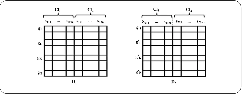
Fig 1: D1, D2 are two different gene expression datasets that have gathered for a specific field of study but by two different settings or techniques. Each column sxyz represents a different sample while subscripts x, y, and z
show the dataset index, class index, and number of samples correspondingly. Rows are genes.
In addition to the above researches, there are lots of papers about the integration of separate microarray studies such as [13-18], these researches more or less, can be categorized as normalization or model building methods.
PROPOSED METHODS
The current paper presents an approach based on the information theory model building. To describe the method, some terminologies are needed to be explained first. Suppose that two separate experiments were done in a same discipline like prostate cancer. But they were performed in two different settings or even with different techniques, and each of which led to separate gene expression datasets D1, and D2. They can be visualized as Fig. 1.
Each row represents a gene and each column shows a sample. There are two classes in each dataset: Cl1=Normal, Cl2=Tumor. The m value is the number of
samples in the class Cl1, and n is the number of samples
in the class Cl2 from D1, while m' and n' are the numbers
of samples in the related classes from D2, respectively.
The total number of samples in D1 is M = m + n, and
M' = m' + n' is the total number of samples in D2. N is
the number of total genes per sample in the datasets D1 and D2. The rows gl and gk show the gene expression
values in D1 while g'l and g'k show expression values of
the same genes in D2.
As, there isn't any presumptions about the equality of noise patterns and settings between two experiments, the equality between probability distribution of any desired
gene gl from the first experiment and its related gene g'l
in the second dataset can't be held even in one class. Particularly, in the case of different standards such as oligo chips for one gene expression dataset and cDNA chip for the other, heterogeneous datasets will be achieved which makes the direct comparison impossible. In this case normalization techniques are very likely to lead to misclassifications.
From here on, gl, gk, g'l, and g'k will be assumed as the
random variables and we will denote them by X, Y, X' and Y' respectively. And these random variables can get different values from their distributions. The D1 will be
supposed as the base dataset, and remains intact.
Background theory
In this subsection we try to prove the following theorem using appendix A.
Theorem1: A similar linear transformation over any two probability distribution of the random variables X and Y (i.e. X' = S.X + c and Y' = s.Y + c), leaves the mutual information intact.
Proof: From information theory concepts [19] mutual information can be defined as:
I(X '; Y ')=H(X ')−H(X ' | Y ') (1) Using above equation and lemma1 and lemma2 from appendix A, we can rewrite it as follow:
[
]
I(X '; Y ')=H(X) log(s)+ − H(X | Y) log(s)− = (2) H(X) H(X | Y)− =I(X; Y)
g1
gL
gK
gN
g'1
g'L
g'K
g'N
D1 D2
s111 ... s11m s121 ... s12n S211 ... s21m s221 ... s22n
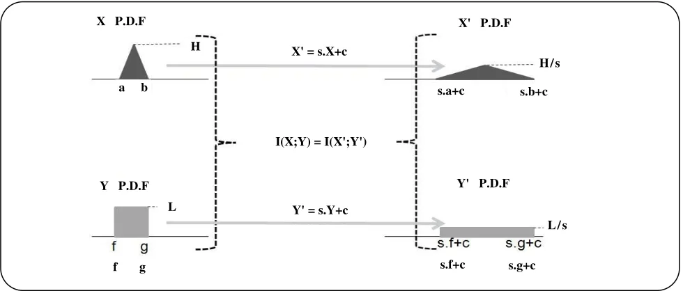
Fig. 2: The Probability Distribution Functions (PDF) of both X and Y are transformed to X', Y' by a desired T. T is described by two quantities s (scaling factor) and c (translation factor) as T(x)=s.x +c. I(X;Y)and I(X';Y')
are mutual information between X, Y, and X', Y', respectively.
Due to the Eq. (2), it is proved that the mutual information between any two random variables remains intact while a similar linear transformation occurs on their distributions.
Proposed validity testing method
As it was said earlier, different labs use different techniques and setups. So, dissimilarity can be seen in the distribution of the gene expressions inside their datasets. Suppose that the distribution of X' is different from X, based on an occurred transformation T; and T is a direct outcome of the different techniques and settings between D1 and D2. In other word, as a result of the
desired transformation T, the same gene has got different distributions in its expression level between D1 and D2.
Fig. 2 shows the idea schematically.
Theorem1 proves that mutual information between any two desired genes' distributions remain intact through different acquisition techniques while any two given genes’ expression distributions have been linearly transformed in a similar manner. In other word, if T is a linear transformation and if it takes effect on the distributions of X, Y to create distributions of X', Y', the mutual information between X, Y and X', Y' will be remained intact (Fig. 2). More than that, we can generalize Eq. 2 to any number of linear transformations. Unfortunately, if mutual information is
intact, T can be linear or non-linear. But according to mathematic formula, a non-linear transformation deforms shapes. So, we are able to implicate in this way: if the mutual information is intact and the shape of the distribution is not deformed, T will be linear. But, as the computational load of shape checking is not something trivial, and both of X and X' are expressions for the same gene in a specific domain of study e.g. prostate cancer, it is supposed that T will be linear if the mutual information is intact.
Now, we are able to use Eq. (2) as a tool for identifying the transformation types between the genes of datasets. Finding any pairs of genes that have linearly transformed helps us to separate genes into two categories: linearly transformed, and non-linearly transformed. It could be done by comparing I(X, Y) any two desired genes from D1,
and I(X', Y') for their corresponding transformed genes in D2. Our validating test process is based on
finding of those genes which are linearly transformed. If there are two desired genes X, Y within D1 and their
transformed genes X', Y' within D2, it could be said that
they are linearly transformed as the followings:
1 2
X, Y D , X ', Y ' D , I(X; Y) I(X '; Y ')
∃ ∈ ∈ = → (3)
(
)
(
)
1 Xk Y
I= = I X; Y I X ; Y′ ′ 0
∆ = − = →
X′=sX+c, Y′=sY+c
X P.D.F X' P.D.F
X' = s.X+c
Y P.D.F Y' P.D.F
Y' = s.Y+c H
H/s
a b
f g
s.a+c s.b+c
L
L/s
s.f+c s.g+c
We call this kind of genes comparable genes. The comparable genes are the ones that are linearly transformed. The value of Ilk represents the difference
between mutual information of two genes l and k from base dataset D1 and mutual information of their corresponding
transformed genes within D2. The comparable genes have
Ilk=0. Eq. 3 could be rewritten for a single gene as:
1 2
X D , X ' D , I(X; X)
∀ ∈ ∈ = (4)
H(X), I(X '; X ')=H(X ')→
l Xk X
I= = log(s) X ' sX c
∆ = → = +
In contrast, incomparability for each pair of different genes can be defined as:
1
X, Y; X, Y D ; X', Y';
∃ ∀ ∈ ∃ ∀ (5)
2
X ', Y '∈D , I(X; Y)≠I(X '; Y ')
Eq. 5 can be used as a robust criterion for omitting noise genes. This equation simply expresses: if there isn't any Y and Y' for a specific X and X' that satisfies Eq. (2), it will be induced that X and X' are not linearly transformed. This means that X, and X' can be omitted and ignored. Due to this fact that the gene compared with all other existing ones is not transformed linearly, and it is disturbed, current expression values of D1,D2 around
this gene is not valid.
Practically, there are lots of noise sources, and there are few samples compared with the number of genes. Hence, using the above exact equations, few or no linear transformed genes can be reported by the Eqs. (3), (4), and (5). So, it is reasonable to compare two datasets, based on these equations somehow not crisply. For example, majority testing for the lowest or highest, putting some threshold, or even establishing of some fuzzy relations instead of the above crisp equations can be used. In this way, we are able to report those genes which are linearly transformed or near to it. We use simple threshold policy in our experiments that is explained in the last section.
Proposed integration method
If the comparable genes are held only in D1 andD2,
they can be easily integrated. As D1 is the base dataset,
the integration can be obtained by inverse transformation over D2. Understanding this, the important job is to find
the scale s, and the translation factor c. This subsection determines equations to help us in this way.
By equations 4 and A-4, scaling factor can be calculated. The following formula is obtained by the equation A-4:
( )
(
)
H(X ') H(X)− =log s → =s exp( H(X ') H(X)− (6)
The quantities of H(X), H(X') are entropies of X, and X' correspondingly. This equation demonstrates the relationship between scaling factor s with the entropy values of a same gene in both datasets D1 and D2.
The translation value ccan be found by checking the same gene expression distributions between two data sets D1 and D2. Suppose that D1 is the reference dataset, and
D2 contains those samples that should be modified in
a way integratable with samples in D1. Finding it,
the expected value of X in D1 and X' in D2, c could be
obtained. The following equation shows relationship between the expected values of the expression distributions and the scaling s with translation factor c.
{ }
{ }
c= Ε X' − Εs X (7)
Two quantities E{X}, E{X'} are the expected values of X, and X' respectively. The values s and c represent scaling and translation factors.
Using s (s≠0) and c, the expression values of X' from D2 can be integrated with D1 as:
~ X ' c X
s −
= (8)
The value X' is a gene expression value in D2, X
is modified gene expression values inversely transformed to integrate with the same gene expression in D1.
As not the whole of genes can exactly be transformed with same s and c as other ones in the practice, there will be vectors for scaling and translation:
{
i}
{
i}
s∈ s ,1≤ ≤i N , c∈ c ,1≤ ≤i N (9) If the values of si are similar and close to each other,
their average can be used instead of different si for each
gene. The same story stands for ci. But if the time of
process isn't too much important, it would be better to work with each si , ci separately.
ALGORITHM
Algorithm 1: The Proposed algorithm for integrating of microarray expression data.
1) Calculate I from samples of one class.
2) Create V by row summation of I.
3) Calculate T.
4) Omit genes lower than T.
5) Calculate s and c for each remained gene.
6) Inverse Translation for each gene.
7) Adding Inverted samples to reference dataset.
Eq. 3 and 4. The indexes l and k represent any two desired genes. Calculating Ilk results in forming
symmetric matrix as:
{
lk}
I I ,1 l N,1 k N
∆ = ∆ ≤ ≤ ≤ ≤ = (10)
1 12 1N
21 2 2N
N1 N2 N N N
log(s ) I I
I log(s ) I
I I log(s ) ×
∆ ∆
∆ ∆
∆ ∆
The value of Ilk is defined as an absolute difference
between mutual information by Eq. (3), so Ilk= Ikl
which is a symmetric matrix. The diagonal value of i-th gene is equal to log(si) calculated by Eq. (4). If the value
of Ilk in any other locations except those in the diagonal
is zero, the l-th and k-th genes are linearly transformed between D1 and D2 with the same s and c. If a value
in diagonal is zero, the corresponding gene is not scaled. In the best case it is a hope to see a zero matrix, meaning X, X' have identical distributions and no transformation has taken effect. As the calculations in this phase takes place for all combination of two genes, it has quadric complexity O(N2) regarding N genes.
As it was mentioned earlier, the Eq. (5) describes a gene which should be omitted. Based on this equation, if the l-th gene has ∆Ilk≠ 0 for all other genes, the l-th gene
shall be omitted. In the matrix of Eq. (10), this can be interpreted as the omittion of those rows that have non-zero values. The more non-zero values the l-th row of the matrix has, the more non-linear characteristics the l-th gene shows. And as the values of Ilk are
non-negative, so the greater summation the l-th row of the matrix has, the more non-linear specifications the l-th gene illustrates.
The merit of a gene omitted is described by the simple threshold in this research. To calculate the threshold
value T, the algorithm performs steps 2, 3 and 4. The second step is about the creation of vector V by I summation in the rows, which is done with the complexity of O(N).
N
i i ij
j 1
V v , (1 i N)v I
=
= ≤ ≤ = ∆ (11)
The third step finds those genes that have vi with
greater values than T, and the fourth step omits them. The threshold value T is calculated by Eq. (12). This equation shows that the one- tenth of the greatest row summation is used as the threshold value in this research. The one tenth is the threshold percentage which was chosen by experiments.
{
i}
T=0.1 Max v ;1 i× ≤ ≤N (12)
In the fifth step, the values s and c are calculated for the remaining genes by the Eqs. (6) and (7). To find s, an exponential function effects on the diagonal values of I matrix. Based on the calculated s and Eq. (7), the translation factor c is calculated.
Step six deals with finding the inverse transformed expression values for the genes by the Eq. (8), and the step seven ends the process by merging the newly calculated values with corresponding genes in D1.
The complexity of phases between 3 and 7, aren't greater than O(N). It makes that the overall complexity of the algorithm will be limited in quadric O(N2) that is suitable in sense of the time to be spent.
EXPERIMENTAL RESULTS
Our experiments fall into two categories: a) finding the threshold percentage, b) performing the whole algorithm on some real datasets.
Finding the threshold percentage
A Random reference dataset D1 was created with
10 features (i.e. genes) whose distributions were selected to be uniform PDF with different mean µ and standard deviation σ. The µ and σ were selected equal to the index of each gene. Creating the modified dataset D2, the initial
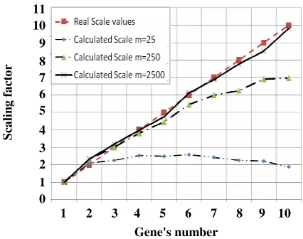
Fig. 3: The results of proposed algorithm in order to find scaling factor (s). Horizontal axis determines the gene number in datasets. Vertical axis shows discovered scaling factor(s). Real effected scaling factors(s) are illustrated by red dashed lined. The other line types and their marks show the discovered (s) which were calculated by different dataset’s number of samples (m). The examined values of m are m=25, 250, and 2500. Each marked point on the discovered values (s) is the average of ten independent runs.
equal to the index of each gene. The number of samples in D1, D2 which is denoted by m, was equal.
As an example, the fourth feature g4 in D1 was created
by sampling a uniform PDF with µ=4 and σ=4 that means g4 ~ (a= -2.9282, b = +10.9282). The distribution
of g'4 in D2 was calculated by a linear transformation
on the PDF of the g4. Due to the scaling and translation
s = c = 4, the g'4 had µ=20 and =16 or in the other word
4
g ' ~(a=-7.7128,b= +47.7128).
In order to discover the threshold percentage, the D1, D2
were fed into the software which was implemented to find the s, c without any threshold value. The software was implemented only based on steps 1 and 5 of the algorithm. The procedure of sampling D1, D2 and looking
for s, c was performed ten times for each dataset’s number of samples m and examined by different values m=25, 250, and 2500.
The discovered results of s and c can be seen in Fig. 3, 4 respectively. The horizontal axis shows the corresponding gene number and the vertical axis represents the corresponding studied values which are the scaling factor s in Fig. 3 and the translation values c in Fig. 4. The discovered values of s and c in Figs. 3 and 4 are the average of ten independent runs of the algorithm.
The Figs. 3 and 4 show some facts. The greater value in the scaling factor s and the translation factor c the gene is affected by, the more deviation in finding the correct values the algorithm has. The deviation can be reduced by increasing the dataset’s number of samples m.
Although, increasing in m makes the discovered values s and c close to the actual values, the number of samples in a real dataset, is fixed and not more than 250 samples. If the relations between the valid values of s, c m are created, the greatest one will be 0.1(i.e. s=2/m=25). It means that we are mostly sure about the deviation beyond this range. In other word, this technique is capable of discovering valid s and c whose values are less than a tenth of the number of samples.
Integration on real datasets
In order to perform the algorithm to do the integration on the real datasets, the prostate cancer microarray datasets which are publicly available were used. These datasets have been presented in some highly valuable papers. For simplicity, each dataset is represented by the abbreviation of the first author of the paper, such as Singh [3], and Welsh [20]. The platform of these datasets is Affymatrix HG-95AV2. Table 1 shows the data-sets’ specifications in brief.
As it is shown, the datasets aren’t equal in their number of genes; so before presenting these datasets within the algorithm, a preparation step is needed in order to balance them. The input datasets and integrated dataset, which is the output of the algorithm, are classified in order to discover the robustness of the algorithm in omitting the noise genes.
Our classification approach for the evaluation is SVM [21] with linear kernel. Despite its complication in adjusting the proper parameters, SVM which works based on machine learning, is a powerful tool not only in the classification tasks but also in the regression and other fields of study. As SVM is a machine learning technique, it is needed to be fed by some samples as the training cases t, and the remaining as the test ones. The Leave One Out Cross Validation (i.e. LOOCV) is used as the training and testing method.
Giving available N samples, LOOCV uses (N-1) samples to build and train the classifier, while the remaining sample inputs are used by the classifier to measure its merit. This process takes place N times and 1 2 3 4 5 6 7 8 9 10
11 10 9 8 7 6 5
4 3 2 1 0
S
ca
li
n
g
f
a
ct
o
r
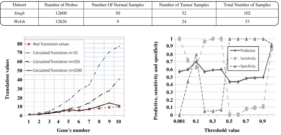
Table 1: The data-sets’ specifications.
Dataset Number of Probes Number Of Normal Samples Number of Tumor Samples Total Number of Samples
Singh 12600 50 52 102
Welsh 12626 9 24 33
Fig. 4: The results of proposed algorithm in finding proper Translation value. Horizontal axis determines the gene number in data sets vertical axis shows effected Translation values to PDF. Real Translation values are illustrated by dashed lined. For example 4th gene has effected by c = 4. The algorithm has found c = 4.2741.
the average of the measured criteria are reported after each time. The evaluated criteria are accuracy, sensitivity, and specificity defined as:
Accuracy = (13)
Sensitivity = (14)
Sensitivity = (15)
The behavior of the algorithm with different threshold values is shown in Fig. 5. It can be seen that increasing the threshold value up to 0.1 makes the predictive accuracy better. Due to the few numbers of samples, threshold values greater than 0.1 make the result worse. Deviation and reduction in predictive accuracy is performed
Fig. 5: The results of proposed algorithm with different threshold values. The vertical axis shows the predictive accuracy, sensitivity, and specificity which are a number between 0 and 1. The horizontal axis is threshold values. Each point is reported by LOOCV.
based on what has been presented previously. If the integration algorithm is performed without any reduction in genes (T=1), SVM will classify the sample with best predictive accuracy.
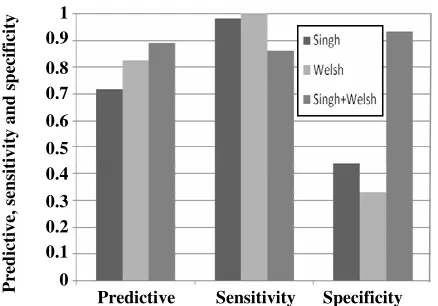
The SVM performance over Singh, Welsh, and the integrated dataset (Singh+Welsh) which is the output of the new integration algorithm without any threshold for reduction, are illustrated in Fig. 6. It shows that the integrated dataset is classified by SVM with highest predictive accuracy and specificity. And the sensitivity is 0.8571 that is less than the others.
Generally speaking, the integrated dataset is classified better than the others. The two out of three evaluated criteria are satisfied by the proposed integration algorithm. Although, its sensitivity is less than the other, but the most important factor in comparison of different methods is predictive accuracy which is satisfied by proposed integration method. It is due to this fact that the algorithm integrating separate datasets creates more relevant samples than any single dataset.
The number of samples that is correctly predicted
The number of total samples
The number of samples that is correctly predicted as tumor
The number of tumor samples
The number of samples that is correctly predicted as Normal
The number of normal samples
1 2 3 4 5 6 7 8 9 10 80
70
60
50
40
30
20
10
0
0.001 0.1 0.3 0.5 0.7 0.9 1
0.9
0.8 0.7
0.6 0.5 0.4
0.3
0.2 0.1
0
T
ra
n
sl
a
ti
o
n
v
a
lu
es
Gene's number
P
re
d
ic
ti
v
e,
s
en
si
ti
v
it
y
a
n
d
s
p
ec
if
ic
it
y
Fig. 6: It shows the classification results over Singh, Welsh, and integrated dataset. The integrated dataset is created by the algorithm without any threshold value. Each result is reported by LOOCV. The vertical axis shows the predictive accuracy, sensitivity and specificity which are between 0 and 1.
CONCLUSIONS
We have presented a new integration method and a validation technique by means of information theory concepts. The method is general for integration of any kind of data whose distributions have been linearly transformed. The validation method is for checking the linearity between two distributions, as the integration method can only cope with linear transformations. Additionally, this article presents new heuristic feature reduction method. The method omits those genes which are not linearly transformed. These methods have been applied in DNA microarray as a special case of their usages. The time complexity of proposed algorithm is in quadric order that is something suitable for practical usages.
APPENDIX A
This assumption will not decrease from the generality of further topics due to this fact that, the number of possible values for each random variable can be increased toward infinite and integral notations can be used instead of sigma form, or one can discreteize these random variables first.
Upon these, we will use some terminology as follow: p(X) and p(Y) are probability mass functions of gl and gk
in D1. And p(X') and p(Y') are probability mass functions
of g'l, g'k in D2, and p(X,Y) is joint probability mass
function of gl, gk and so on. p(xi) is probability of
a specific event xi out of an events' list that is related to
random variable X and l is number of these events. p(yj)
and p(xi,yj) are similarly defined, m is possible number of yj.
Suppose a given gene as a discrete random variable X that can get different possible values {x1,..,xl} and c,s∈ℜ,
are scaling and translation factors that scale and transform a given gene's expression distribution uniformly between D1 and D2. Thus it can be written as follow:
i i 1 l
0≤p(x )≤1, x ∈X≡{x ,..., x }, (A-1)
l
X ' sX c i
i 1
p(x ) 1 = +
=
= →
i i 1 sl
0≤p(x ')≤1, x '∈X '≡{x ',..., x '},
sl c
i
i i
i 1 c
p(x ) p(x ') 1 p(x ')
s
+
= +
= → =
j j 1 m
0≤p(y )≤1, y ∈Y≡{y ,..., y }, (A-2)
m
Y ' sY c j
j 1
p(y ) 1 = +
=
= →
j j 1 sm
0≤p(y )≤1, y ∈Y '≡{y ',..., y '}, sm c
j
j j
j 1 c
p(y ) p(y ') 1 p(y ')
s
+
= +
= → =
Lemma1: Linear transformation X'=sX+c over a random variable increases the total ambiguity equal to logarithm of effected scaling factor.
Proof: Entropy of random variable X can be calculated upon its definition [19] and Eq. (1) as follow:
l
X ' sX c
i i
i 1
H(X) p(x ) log(p(x )) = +
=
= − → (A-3) sl c
i i
i 1 c
H(X ') p(x ') log(p(x '))
+
= +
= −
Using index shifting, A-1, and A-2 we are able to change it as follow:
sl
i i
i 1
H(X ') p(x ') log(p(x '))
=
= − = (A-4) sl
i i
i 1
p(x ) p(x )
log( )
s s
=
− =
sl sl
i 1 i 1
1
p(x) log(p(x)) p(x) log(s)
s − = + = =
[
]
1
sH(X) s log(s)
s + = H(X) log(s)+
Example: We have a dice with six faces, the total ambiguity or entropy is 2.5849(bit). If a special 12 faces dice is designed, the entropy would be equal to 3.5849(bit), equation A-4 is hold with the scaling factor 2.
Lemma2: Linear transformations X'=sX+c and Y'=sY+c over two random variables increase the conditional entropy equal to logarithm of effected scaling factor.
Proof: For conditional entropy we can write as follow: l m
i j i j
i 1 j 1
H(X | Y) p(x , y ) log(p(x | y ))
= =
= − = (A-6)
l m
i j i j
j i 1 j 1
p(x , y ) p(x , y ) log( )
p(y )
= =
−
H(X ' | Y ')=
sl c sm c
i j i j
j i 1 c j 1 c
p(x ', y ')
p(x ', y ') log( )
p(y ')
+ +
= + = +
−
For joint probability we have the following relationship:
i i j j
X ' sX c,Y ' sY c,x X,x ' X ',y Y,y ' Y ' i j
p(x , y )→= + = + ∈ ∈ ∈ ∈ (A-7)
i j
i j 2
p(x , y ) p(x ', y ')
s
=
From joint entropy definition we have:
H(X, Y)=H(Y) H(X | Y)+ = (A-8)
l m
i j i j
i 1 j 1
p(x , y ) log(p(x , y ))
= =
Based on the above equations A-2, A-6, A-7, and using index shifting it could be written:
sl sm
i j i j
2
j i 1 j 1
p(x , y ) p(x , y )
H(X ' | Y ') log( )
s s.p(y )
= =
= − = (A-9)
sl sm
i j i j
2 i 1 j 1 1
p(x , y ) log(p(x , y ))
s = =
−
−
sl sm
i j j
i 1 j 1
p(x , y ) log(s.p(y ))
= = = sm 2 j j 2 j 1 1
s H(X, Y) s. p(y ) log(s.p(y ))
s + = =
sm sm
2
j j j
2
j 1 j 1
1
s H(X, Y) s. p(y ) log(s) s. p(y ) log(p(y )
s + = + = =
2 2 2
2 1
s H(X, Y) s log(s) s H(Y)
s + − =
H(X, Y) log(s) H(Y)+ − =H(X | Y) log(s)+
Received : March 15, 2010 ; Accepted : Jan. 17, 2011
REFERENCES
[1]
Iyer V.R. et al., The Transcriptional Program in the Response of Human Fibroblasts to Serum, Science, 283, 83, (1999).
[2] Choi J.K., Yu U., Kim S., Yoo O.J., Combining Multiple Microarray Studies and Modeling Interstudy Variation, Bioinformatics, 19, p. 84, (2003).
[3] Singh D. et al., Gene Expression Correlates of Clinical Prostate Cancer Behavior, Cancer Cell, 1, p. 203 (2002).
[4] Chen W.B., Zhang C., Liu W.L., An Automatic and Robust Method for Microarray Image Analysis and the Related Information Retrieval for Microarray Databases, "(ICDE 2007) IEEE 23rd International Conference", 85 (2007).
[5] Katzer F.K.M., Methods for Automatic Microarray Image Segmentation, IEEE Transactions on nanobioscience, 2, p. 202 (2003).
[6] Knudsen S., "Guid to Analysis DNA Microarray Data", John Wiley, (2007).
[7] Conde L., Mateos A., Herrero J., Dopazo J., Unsupervised Reduction of the Dimensionality Followed by Supervised Learning with a Perceptron Improves the Classification of Conditions in DNA Microarray Gene Expression Data, "Neural Networks for Signal Processing", 77 (2002).
[8] Huang T.-M., Kecman V., Kopriva I., Feature Reduction with Support Vector Machines and Application in DNA Microarray Analysis, "Kernel Based Algorithms For Mining Huge Data Sets", Springer, 95 (2007).
[9] Lai Y., Eckenrode S.E., She J., A Statistical Framework for Integrating Two Microarray Data Sets in Differential Expression Analysis, "17th Asia Pacific Bioinformatics Conference (APBC2009)", (2009).
[10] Jiang H. et al., Joint Analysis of Two Microarray Gene-Expression Data Sets of Select Lung adenocarcinoma marker genes, BMC Bioinformatics, 5, p. 8 (2004).
[12] Kang J., Yang J., Xu W., Chopra P., Integrating Hetrogeneous Microarray Data Sources using Correlation Signatures, Data Integration in the Life Sciences (DILS),3615/2005, p. 105 (2006).
[13] Xu L., Tan A., Naiman D., Geman D., Winslow R., Robust Prostate Cancer Marker Genes Emerge from Direct Integration of Inter-Study Microarray Data, Bioinformatics, 21, p. 3905 (2005).
[14] Conlon E., Song J., Liu J., Bayesian Models for Pooling Microarray Studies with Multiple Sources of Replications, BMC Bioinformatics, 7, p. 247, (2006).
[15] Hong F., A Comparison of Meta-Analysis Methods for Detecting Differentially Expressed Genes in Microarray Experiments, Bioinformatics, 24, p. 374, (2008).
[16] Xu L., Tan A., Winslow, R. Geman D., Merging Microarray Data from Separate Breast Cancer Studies Provides a Robust Prognostic Test, BMC Bioinformatics, 9, p. 125 (2008).
[17]Borozan I. et al., MAID: An Effect Size Based Model for Microarray Data Integration Across Laboratories and Platforms, BMC Bioinformatics, 9, p. 305 (2008).
[18] Cahan P. et al., List of Lists-Annotated(LOLA): a Database for Annotation and Comparison of Published Microarray Gene Lists, Gene, 360, p. 78 (2005).
[19] Cover T.M., Thomas, J.A., "Elements of information theory", Wiley, (2006).
[20] Welsh J.B. et al., Analysis of Gene Expression Identifies Candidate Markers and Pharmacological Targets in Prostate Cancer, Cancer Research, 61, p. 5974 (2001).