Computationally optimizing the directed evolution of proteins

Proteins

Thesis by

Christopher Ashby Voigt

In Partial Fulfillment of the Requirements for the Degree of Doctor of Philosophy

California Institute of Technology Pasadena, California, USA

2002

© 2002

Abstract

Acknowledgements

Just before I started writing my thesis, I imagined that I would probably write the title page, copyright page, an over-ambitious table of contents, and acknowledgements first. I would then procrastinate for the next six months in putting together the bulk of the writing. In reality, the thesis has come together in the opposite way. I have found writing the acknowledgements to be much more difficult than expected, and this has been compounded as I put each chapter together and remember the enormous group of people that have made this possible.

Foremost, I need to acknowledge my three advisors at Caltech (in order of appearance): Zhen-Gang Wang, Frances Arnold, and Stephen Mayo. They provided a wonderful collaborative environment, which gave me the freedom to explore different ideas. I am grateful for the unique training in theoretical, computation, and experimental methods that they provided. Working with them has made for a very enjoyable graduate experience.

with Deepshikha Datta in trying to discover structural switches in proteins. From the Wang group, I have had many stimulating conversations on the dynamics of polymers with Andy Spakowitz.

Over time, I have interacted with many new and old members of the three groups. Their ideas have subtly altered the direction of my research interests. In the Mayo group, I would like to thank Oscar Alvizo, Julie Archer, Mary Ary, Dan Bolon, Cynthia Carlson, Eun Jung Choi, Deepshikha Datta, Geoffrey Hom, Possu Huang, Shira Jacobson, Caglar Tanrikulu, Kirsten Lasilla, John Love, Jessica Mao, Andrei Marinescu, Shannon Marshall, Chantel Morgan, J. J. Plecs, Scott Ross, Cathy Sarisky, Julia Schifman, Premal Shah, Pavel Strop, and Eric Zollars. A special thanks goes to Dr. Love for teaching me the sins of Vegas and taking my money. Luckily, Possu, Geoff, and Premal were also playing so I could ultimately break even. Currently, Peter Samuelson, a freshman, is programming Web applications based on this thesis. He will probably be done before I finish writing this. The lab would not run nearly as smoothly if it were not for Cynthia Carlson. She made everything come together. Finally, Darryl Willick, Ryan Martin, and Hezekiah McMurray need to be thanked for their behind-the-scenes work to keep the computers running.

Hiraga, John Joern, Oliver May, Kimberly Mayer, Peter Meinhold, Kentaro Miyazaki, Michelle Meyer, Peter Nguyen, Chris Otey, Ioanna Petrounia, Claudia Schmidt-Dannert, Rebecca Schulman, Uli Schwaneberg, Volker Sieber, Jonathan Silberg, Lianhong Sun, Todd Thorson, Alex Tobias, Andrew Udit, Daisuke Umeno, Alex Volcov and Yohei Yokobayashi. I should thank John Joern for letting me live with him, which is not a minor thing if you have seen my office. During recruitment, Pat Cirino convinced me to come to Caltech and has subsequently stomached my rants regarding graduate life.

Niles Pierce has played an active role in my graduate career, both as a postdoc in the Mayo lab and as a professor. I particularly appreciate advice that he gave me in using Matlab and applying for jobs. His wife, Gillian, was very helpful in editing a large book chapter that I wrote. Near the end of my time here, I have gotten to know one of his students, Robert Dirks, mostly through his pervasive use of computer time.

Beyond the SFI, I have collaborated with researchers at other institutions. Dane Wittrup at MIT is one of the first people to test the ideas in this thesis on creating libraries on antibodies (Chapter 4). His student, Brenda Kellogg, was responsible for lab work for this project. I have also collaborated with Jim Bull, George Georgiou, and Brent Iverson at the University of Texas, Austin. Their ability to produce massive amounts of data inspired some of the work presented here.

Prior to graduate school, there were numerous teachers and professors that had very positive and influential roles. When I was a student at Brandywine High School, Ronald Eschelman managed to motivate me in chemistry. In addition, I was inspired by Vincent Pro (history), Jeff Stugard (drafting), and Tom Twilley (biology). At the University of Michigan, Robert Ziff introduced me to statistical mechanics, and more importantly, the concept of doing research. While I was still at Michigan, I met Richard Goldstein in the biophysics research division. Through his language and colorful use of analogies, Richard has greatly influenced my speaking style.

Table of Contents

Abstract iii

Acknowledgements iv

Table of Contents ix

List of Tables xi

List of Figures xii

Chapters

Chapter 1 1-1

Introduction to Directed Evolution Theory

Chapter 2 2-1

Modeling the Dynamics of Directed Evolution

Chapter 3 3-1

Targeting Mutagenesis with Structural Information

Chapter 4 4-1

Tolerance of the CDRs of Antibody D1.3

Chapter 5 5-1

Recombination Preserves Protein Building Blocks

Chapter 6 6-1

Comparing Search Algorithms in Protein Design

Chapter 7 7-1

Evolvable Systems in Biology

Appendixes

Appendix A A-1

Higher-Order Moments of the Mutant Distribution

Appendix B B-1

Dead-End Elimination and Monte Carlo Entropy Calculations

Appendix C C-1

Adding Ambient Temperature to the Sequence Entropy

Appendix D D-1

Appendix E E-1 Combinatorial Libraries Based on Schema Disruption

Appendix F F-1

Non-homologous Recombination

List of Tables

Table 1-1: Discovery times for evolutionary algorithms

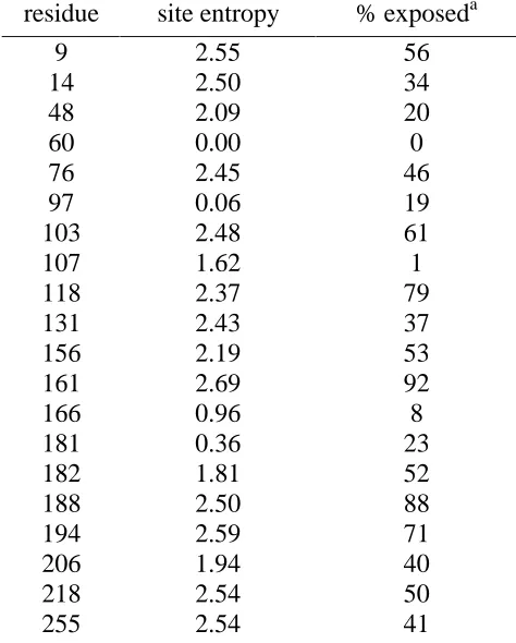
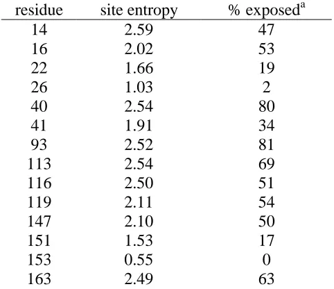
Table 3-1: Site entropies and solvent accessibility of subtilisin E Table 3-2: Site entropies and solvent accessibility of T4 lysozyme Table 3-3: Saturation of high-entropy residues ofβ-lactamase Table 4-1: Full ORBIT sequence design of CDR residues Table 4-2: ORBIT design of targeted residues

Table 4-3: Comparison of experimental and computational results Table 5-1: Designed TEM-1/PSE-4 hybridβ-lactamases

Table 6-1: Overview of the 20 protein test set

Table 6-2: Results of side chain placement calculations Table 6-3: Times for side chain placement calculations

Table 6-4: DEE explosion behavior for protein sequence designs Table 6-5: Core results for sequence design calculations

List of Figures

Figure 1-3: A cartoon of the fitness landscape

Figure 1-4: Searching smooth and rugged landscapes Figure 1-5: Mutational constraints in protein structures Figure 1-6: Constraints lead to a decrease in entropy Figure 1-7: Mutational capacity of different words Figure 1-8: A schematic of protein design tools

Figure 1-9: Recombination accelerates word construction

Figure 2-1: Optimal mutation rates based on evolutionary parameters Figure 2-2: Beneficial mutations are biased towards uncoupled residues Figure 2-3: A transition for discovering compensating mutations

Figure 2-4: Modeling the mutant distribution

Figure 2-5: The mean and standard deviation of the mutant distribution Figure 3-1: Sequence entropy versus stabilization energy

Figure 3-2: Sequence entropy freezes at high fitness

Figure 3-3: Sequence entropy and solvent accessibility of subtilisin E

Figure 3-4: Entropy mapped onto the structures of subtilisin E and T4 lysozyme Figure 3-5: Beneficial mutations occur at high sequence entropy residues Figure 3-6: Activity improvement versus sequence entropy for T4 lysozyme Figure 3-7: Average sequence entropy versus generation for antibody 4-4-20 Figure 3-8: Comparison of entropy, solvent accessibility, and natural diversity Figure 3-9: Sequence entropy versus functional tolerance

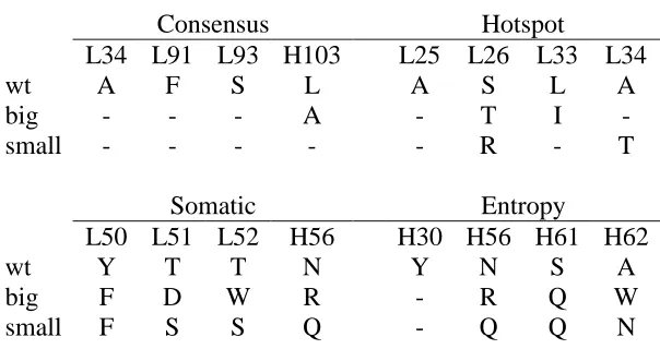
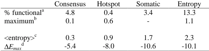
Figure 3-10: Mutated high entropy residues ofβ-lactamase Figure 4-1: Structure of antibody D1.3 bound to HEL Figure 4-2: Full sequence design of CDR residues Figure 4-3: Partial sequence design of targeted residues Figure 4-4: The sequence entropies of the CDR residues

Figure 4-5: The CDR entropies mapped onto the D1.3 structure Figure 4-6: The entropy versus distance from binding interface Figure 4-7: The residue entropies with and without solvation Figure 5-1: An illustration of schema disruption

Figure 5-2: Calculating the probabilities for broken interactions

Figure 5-3: Comparison of schema disruption profiles with recombination data Figure 5-4: Single-crossover disruption profile for GART

Figure 5-5: Schema disruption profile for TEM-1/PSE-4β-lactamase Figure 5-6: Schema mapped onto theβ-lactamase structure

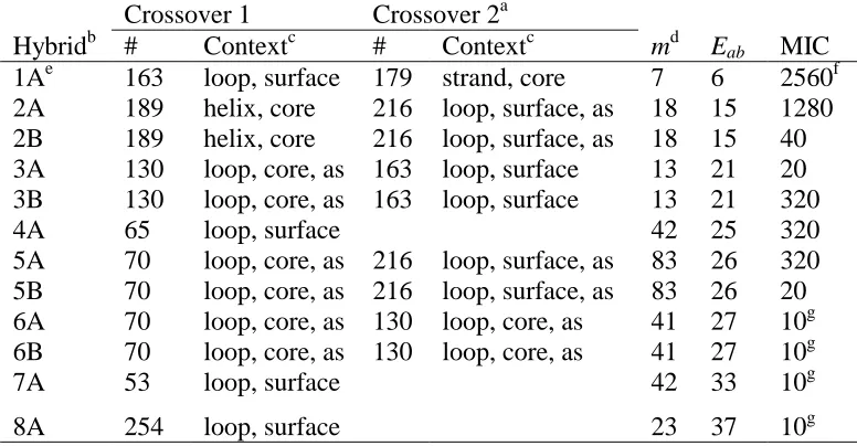
Figure 5-7: Interactions between schema Figure 5-8: Designed TEM-1/PSE-4 hybrids

Figure 5-10: The parameter sensitivity of the schema disruption profile Figure 5-11: The effect of parental identity on the schema disruption profile Figure 5-12: The schema disruption profile and other domain algorithms

Figure 6-1: The fraction of incorrect rotamers found by various search algorithms Figure 6-2: The energy difference between the GMEC and other solutions

Figure 6-3: Convergence time for DEE versus number of design positions Figure 6-4: MCQ and SCMF results for core, boundary, and surface designs Figure 7-1: Robustness and evolvability in parameter space

Figure 7-2: Robust and fragile architectures of nodes and edges Figure 7-3: A comparison of knock out graphs for protein libraries Figure 7-4: The segment polarization network of Drosphila

Figure 7-5: The range of carotenoids produced by directed evolution Figure B-1: A schematic of the DEE-entropy algorithm

Figure B-2: Comparing mean-field and DEE calculated sequence entropies Figure B-3: An example of Monte Carlo output

Figure B-4: Comparing mean-field and Monte Carlo calculated sequence entropies Figure D-1: A cartoon of the mapping between sequence and structure space Figure D-2: The joint sequence entropies for protein G and engrailed

Figure D-3: Common allowed amino acids for protein G and engrailed Figure E-1: Designed TEM-1/PSE-4 libraries with targeted crossovers Figure E-2: Fraction of low-disruption hybrids in targeted libraries Figure E-3: Low-disruption hybrids from the MIN and MAX libraries Figure E-4: Low-disruption hybrids from the MIN-MAX library Figure E-5: Experimental results for the MIN-MAX library Figure E-6: Properties of random seven-crossover libraries

Figure E-7: Comparison of random libraries and the schema profile Figure F-1: β-lactamase schema without the probability matrix Figure F-2: Schema abundance in protein structure database Figure F-3: Non-homologous structure withβ-lactamase schema Figure F-4: Structural alignments of schema 1+2

Chapter 1

Introduction to Directed Evolution Theory

Enzymes can catalyze a wide range of difficult reactions with high specificity in mild conditions. Despite these advantages, it is difficult to coax enzymes to work on an industrial scale (Thayer, 2001). Enzymes may have low activity towards desired, non-natural reactions and they are often destabilized by reactor conditions, such as high temperatures and organic solvents. It is desirable to optimize enzymes to reduce their disadvantages while retaining their beneficial properties. However, the development of reliable enzyme-modification methods is limited by multiple competing constraints in proteins. For example, a change that improves activity may reduce some other desired property, such as the stability or expression yield. An approach to this problem is to reproduce evolution in vitro, through iterative rounds of mutation and selection (Figure 1-1). Within this approach, there is potential for optimization based on principles gleaned from statistical mechanics, computer science, and protein design. The focus of this thesis is the development of computational techniques to model and accelerate the directed evolution of enzymes.

Those properties that incur survival in evolution are collectively referred to as the protein’s fitness.

During evolution, nucleotide mutations are made spontaneously in the DNA of genes, which translate into amino acid substitutions in proteins. Those mutations that are either neutral or lead to an increase in fitness survive, whereas those mutants that have decreased fitness die. This process can be visualized as a random walk through sequence space – the hyper-dimensional set of all possible amino acid combinations, connected via single amino acid substitutions. A useful analogy in understanding sequence space is the concept of a word space (Figure 1-2) (Smith, 1970). In this space, words are connected by single letter substitutions and movements can be made if the substitution results in an English word. Similarly, mutations can cause drift in sequence space along paths where the intermediate sequences are adequately fit to survive selection.

In proteins, rugged landscapes arise from competing interactions between residues (Figure 1-5). For example, if the side-chains of two amino acids interact, then mutating either residue first may lead to a disruption of the interaction and a decrease in fitness (Baase et al., 1999). However, if both residues are mutated simultaneously, then this has the potential of replacing the interaction entirely, thus improving the likelihood of increasing the fitness. Another way to describe this scenario is to note that the sum of the individual changes in fitness is not equal to the change in fitness of the two mutations made simultaneously. This effect is referred to as non-additivity and it reflects the fact that the residues are interacting. This interaction leads to ruggedness in the fitness landscape and makes the search problem more difficult for evolutionary techniques.

Models have been developed in statistical mechanics to describe the effect of competing interactions on the set of energetic states of a system. In particular, spin-glasses, where the interactions between the spin states of atoms contribute to the ground state of the system, have been extensively studied (Sherrington and Kirkpatrick, 1975; Fischer and Hertz, 1991). Because of their ability to capture competing constraints on biomolecules, these simplified models have been used to study the dynamics of evolution (Anderson, 1983; Prügel-Bennet and Shapiro, 1994). In Chapter 2, a spin-glass-like model is introduced to study the effect of inter-residue interactions on the optimal evolutionary parameters.

and right-hand sides with equal probability. When the molecules are restricted to the left-hand side through the addition of a restraint, this reduces the number of states toΩL. The

change in entropy∆S is

      Ω Ω − = − = ∆ L L S k S

S ln , (1-1)

where k is Boltzman’s constant. By dramatically decreasing the number of available

states, the introduction of a restraint can significantly reduce the entropy of a system. The

addition of a constraint can be thought of as the reduction or removal of a potential

barrier or free energy (Hill, 1960).

The reduction of entropy through the introduction of constraints can be

demonstrated by returning to the concept of word space (Shannon, 1951; Abramson,

1963). Considering two different starting points -WORD and ALSO- the number of

single-mutant neighbors that are also English words can be enumerated (Figure 1-7 A).

Due to the spelling rules of English, some of the letters are more easily substituted.

Based on the alignment of words, the entropy of each position can be calculated (Figure

1-7 B). In terms of proteins, constraints are imposed at each residue by the particular

three-dimensional topology of the backbone and interactions with other amino acids.

These constraints restrict the number of amino acids that can be substituted at each

position.

While the statistical models have proven useful in understanding the generalized

dynamics of evolution, their simplicity impedes their ability to model specific enzymatic

systems. To achieve this, more realistic energies have to be calculated based on the

tools (Figure 1-8). The original goal of protein design is computationally optimize an

amino acid sequence to fold into a defined three-dimensional structure (Hellinga and

Richards, 1994; Desjarlais and Handel, 1995; Dahiyat and Mayo, 1997b). The first step

of protein design is to reduce the conformational complexity of amino acids by assigning

a set of discrete rotamers for each amino acid at each residue. Then, all of the interaction

energies between all pairs of rotamers are calculated. Finally, a minimization algorithm is

used to find the amino acid sequence that has the lowest predicted energy in the folded

state of the protein. These techniques are valuable in modeling molecular evolution

because they can be used to calculate the constraints between amino acids for a particular

three-dimensional structure. This facilitates the prediction of the evolutionary dynamics

for experimentally relevant systems, as is done in Chapter 3.

The recombination of several homologous sequences has proven a successful

strategy for directed evolution (Stemmer, 1994; Crameri et al., 1998). This technique

creates a library of hybrid genes where each mutant has inherited portions of their genetic

material from different parents. The power of recombination can be demonstrated by

considering the construction of a library of sentences (Figure 1-9). Recombination

promotes word swapping whereas mutations alone are more likely to destroy the integrity

of a word. The utility of recombination as a search technique has been studied

extensively in computer science (Holland, 1975; Mitchell, 1992). An interesting result

from these studies is that crossovers are not universally advantageous for all search

problems (Schaffer and Eschelman, 1991; Spears and De Jong, 1991; Mühlenbein, 1992).

In fact, they have often been shown to hinder the search (Table 1-1) (Mitchell et al.,

(Manderick et al., 1991; Kauffman, 1993; Hordijk and Manderick, 1995; Voigt et al.,

2001). When crossovers do not divide the constraints of a system, then recombination is

more likely to be successful. In the case of a sentence, this means that crossovers should

occur between words. In protein evolution, crossovers should not divide interactions

between amino acids. Methods to identify regions of protein structures where crossovers

are likely to disturb interacting residues are presented in Chapter 5.

There are several future goals in expanding the development of computational

tools for directed evolution. Foremost, the targeting strategies proposed here have to be

assessed for their ability to accelerate the discovery of novel enzymatic properties. In

constructing enriched libraries, two conditions need to be optimized. First, the

destabilizing effects of mutations and crossovers have to be minimized. Second, the

diversity of the library should be maximized. Balancing these two factors is nontrivial

and could be aided by techniques borrowed from multi-objective optimization (Loughlin

and Ranjithan, 1997). A second goal is to extend directed evolution theory to model and

optimize the evolution of genetic circuits and metabolic networks (Cremeri et al., 1997;

Schmidt-Dannert et al., 2000). Models of biochemical networks can be used to identify

those components that are most likely to generate diverse network functions when

mutagenized. By expanding the theory to explore the evolution of different hierarchies in

biology, it may be possible to develop an understanding of the organizational strategies

Table 1-1. Discovery Times for Evolutionary Algorithms

Algorithma Timeb Steepest ascent hill-climbingc >265,000 Random mutation hill-climbingd 6179 Genetic algorithme 61334

a. Algorithms and data taken from Mitchell (1992).

b. The mean number of function evaluations required to find the optimal string for a “royal road” fitness landscape, averaged over 200 landscapes.

c. An initial string is chosen at random. All single mutations are attempted and the most fit mutant becomes the next parent. This process is repeated until no more fit mutations are found.

d. An initial string is chosen at random. Mutations are randomly attempted and the first mutant that has an increased fitness becomes the next parent. This process is repeated until convergence is achieved.

e. Two initial strings are chosen at random and a population of offspring is produced with crossover rate pc and mutation

rate pm. Selection pressure is then applied to the population.

Figure 1-1:

A schematic is shown of the directed evolution algorithm with potential areas for

optimization marked in red. The first step of directed evolution is to isolate the DNA

sequence that encodes the wild-type protein. Through PCR techniques, a library of

mutant or recombinant DNA sequences is produced. Each member of this library has a

sequence that is slightly perturbed from the parent. This library is then screened for those

properties in which the researcher is interested. The mutant with the best combination of

properties (highest fitness) becomes the parent to the next round of mutation and

selection. Within the directed evolution algorithm, there is much potential for

optimization. The evolutionary parameters are interdependent, for example, the optimal

mutation rate depends on the screening capacity. Further, after each generation, the list of

mutant fitnesses contains information about the local search space. Rather than discarding

this information, it is desirable to use it to optimize the evolutionary parameters for the

next generation. Finally, information, such as the three-dimensional structure of the

protein or alignments of naturally occurring sequences, is being rapidly accumulated for

many enzymatic systems. This information has the potential to optimize the evolutionary

wild-type sequence

mutation recombination

screen and sort mutants according to fitness top mutant

becomes parent of next generation

mutant #

Fi

tn

es

s

1,000 to 1,000,000 mutants

Less-fit mutants are discarded Rate, fragment size,

optimal locations

Screening Size, Proactive use of landscape Data

External Information

Structure Natural Alignments

Figure 1-2:

Transitions between words are similar to movements through sequence space (Smith,

1970). In this example, WORD is transformed into GENE via two paths consisting of

single letter substitutions. A requirement is that each intermediate set of four letters

composes an English word. Two independent paths are shown. The probability that a

transition will occur between two sequences during evolution is related to the number of

WORD

WORE

GORE

GONE

GENE

WOND

WONE

Figure 1-3:

A two-dimensional projection of the hyper-dimensional fitness landscape is shown. In

this simplified representation, for a four-residue sequence is considered where the colors

represent amino acid identities. The all-blue sequence is the global optimum whereas the

lower fitness peaks are local optima. The problem of in vitro evolution is how to search

{Sequence Space}

Fit

n

es

Figure 1-4:

An example is shown of a smooth (A) and rugged (B) fitness landscape. Rugged landscapes are characterized by multiple maxima, which act as traps for an evolving

sequence. Conversely, a smooth landscape contains fewer such peaks. Hypothetical

random starting points are marked by the red dots. From any starting point, the smooth

landscape is easy to climb. Any algorithm of mutagenesis of selection is guaranteed to

discover the global optimum. However, it is more difficult to optimize a sequence on a

rugged landscape, as a steepest-ascent mutagenesis algorithm is likely to converge onto a

Sequence Space

Fi

tn

e

s

s

Sequence Space

Fi

tn

e

s

s

(A)

Figure 1-5:

A simple example is shown that demonstrates constraints in the protein structure. In this

example, a particular set of two mutations leads to an increase in fitness. However, if

either mutation is made individually, this leads to a decrease in fitness (here, due to the

over- or under-packing of atoms). Another way to describe this scenario is to note that the

sum of the individual changes in fitness is not equal to the change in fitness of the two

Wild-type

Improved Mutant AB Intermediate Mutant A

Intermediate Mutant B

Fitness↓

Figure 1-6:

The box shown contains ten freely diffusing molecules. In this simplification, each

molecule can exist in either one of two states: the left or right of the box (demarcated by

the dashed gray line). When the molecules are allowed to diffuse freely, the probability

that each molecule will exist on either side is 0.5. When a barrier is imposed on the

system, the probabilities change to either 1.0 or 0.0 and the entropy of the system

decreases. This example was inspired by a presentation by Jeffrey Saven (University of

Figure 1-7:

(A) The sets of four letters attainable with single substitutions from WORD and ALSO. Those sets that correspond to English words are marked in red. The first and last letters

in WORD are variable whereas the middle letters and the letters of ALSO are less

mutable. (B) Based on the alignment in (A), the entropy of each position can be calculated. Low entropies indicate intolerance to substitutions due to constraints. Here,

the constraints are the spelling rules of English. In protein structures, the constraints are

WORD

AORD

BORD

CORD

DORD

EORD

FORD

GORD

HORD

IORD

JORD

KORD

LORD

MORD

NORD

OORD

PORD

QORD

RORD

SORD

TORD

UORD

VORD

XORD

YORD

ZORD

WORD

WARD

WBRD

WCRD

WDRD

WERD

WFRD

WGRD

WHRD

WIRD

WJRD

WKRD

WLRD

WMRD

WNRD

WPRD

WQRD

WRRD

WSRD

WTRD

WURD

WVRD

WWRD

WXRD

WYRD

WZRD

WORD

WOAD

WOBD

WOCD

WODD

WOED

WOFD

WOGD

WOHD

WOID

WOJD

WOKD

WOLD

WOMD

WOND

WOOD

WOPD

WOQD

WOSD

WOTD

WOUD

WOVD

WOWD

WOXD

WOYD

WOZD

WORD

WORA

WORB

WORC

WORE

WORF

WORG

WORH

WORI

WORJ

WORK

WORL

WORM

WORN

WORO

WORP

WORQ

WORR

WORS

WORT

WORU

WORV

WORW

WORX

WORY

WORZ

5

1

1

5

ALSO

BLSO

CLSO

DLSO

ELSO

FLSO

GLSO

HLSO

ILSO

JLSO

KLSO

LLSO

MLSO

NLSO

OLSO

PLSO

QLSO

RLSO

SLSO

TLSO

ULSO

VLSO

WLSO

XLSO

YLSO

ZLSO

ALSO

AASO

ABSO

ACSO

ADSO

AESO

AFSO

AGSO

AHSO

AISO

AJSO

AKSO

AMSO

ANSO

AOSO

APSO

AQSO

ARSO

ASSO

ATSO

AUSO

AVSO

AWSO

AXSO

AYSO

AZSO

ALSO

ALAO

ALBO

ALCO

ALDO

ALEO

ALFO

ALGO

ALHO

ALIO

ALJO

ALKO

ALLO

ALMO

ALNO

ALOO

ALPO

ALQO

ALRO

ALTO

ALUO

ALVO

ALWO

ALXO

ALYO

ALZO

ALSO

ALSA

ALSB

ALSC

ALSD

ALSE

ALSF

ALSG

ALSH

ALSI

ALSJ

ALSK

ALSL

ALSM

ALSN

ALSP

ALSQ

ALSR

ALSS

ALST

ALSU

ALSV

ALSW

ALSX

ALSY

ALSZ

0

0

1

0

(B)

0.0

0.5

1.0

1.5

2.0

1

2

3

4

W ORD

ALSO

Position

En

tr

o

p

Figure 1-8:

The typical set of computational tools for protein design is shown schematically. First,

the three-dimensional structure is retrieved and the side chains are stripped, leaving a

fixed backbone structure. Then, each residue is classified as existing in the core,

boundary, or surface of the protein. Only hydrophobic amino acids are allowed in the

core, hydrophilic amino acids at the surface, and all amino acids in the boundary. The

flexibility of the amino acid side chains is captured using a set of discrete conformational

rotamers. Next, all of the side-chain/side-chain and side-chain/backbone energies are

calculated using a force field that includes terms for solvation, H-bonding, electrostatics,

and van der Waals interactions. Finally, the optimal set of rotamers is obtained using a

search algorithm, such as dead-end elimination or Monte Carlo simulated annealing (see

fixed backbone designate sidechains: core

boundary surface

Build energy matrix of sc/bb and sc/sc

interactions

Search energy landscape for sequence that best fits into the structure

pairs

single

E

E

E

=

+

define rotomers:

hydrophobic core

hydrophilic surface

everything in boundary LEGAALIYGALLKLYGKKL

{sequence/rotomer space}

En

er

g

y

2 1

3

Figure 1-9:

(A) From a partial starting sentence, point mutations are unlikely to discover new sentences because the number of simultaneous mutations required is too large to be

sampled in a reasonable amount of time. The vast majority of single- or

multiple-substitution sentences will be nonsensical. (B) If recombination is allowed to swap the words from two sentences, then it is more likely to create a library of potentially new

sentences. However, if recombination is allowed to divide the words, the library will be

THE HRAD AND IN A FRONTAL ATTACK

THE HEAD AND IN A FOONTAL ATTACK

THE HEAD ANT IN A FRONTAL AUTACK

THE HEAD AND IN T FRONTAL ATTACK

THEXHEAD AND IN A FRONTAL ATTACK

THE HEMD AND IN A FRONTAL ATTACK

THE HEAD AND IQ A FRONTAL ATTACK

THE HEAD AND IN A FRONTPL ATTACK

THE HEAD AND IN I FRONTAL ATTACK

THE HRAD AND IN A FRONTAL ATTACK

THE HEAD AND IN A FRONTAL ATTACK

THE HEAD AND IN A FRONTAL ATTACK

THIS POINT IS THEREFORE METHOD

THIS POINT IN A FRONTAL ATTACK THE HEAD AND THEREFORE METHOD

THIS HEAD AND IN A METHOD ATTACK

THIS POINT IN A FRONTAL METHOD

THE POINT IS THEREFORE ATTACK

THIS POINT IN A FRONTAL METHOD

THE HEAD AND IS THEREFORE METHOD THIS HEAD IS THEREFORE ATTACK THE HEAD POINT IS THEREFORE

THIS POINT AND IN A FRONTAL ATTACK

(A)

Chapter 2

Modeling the Dynamics of Directed Evolution

Portions of this chapter are reproduced from:

Voigt, C. A., Mayo, S. L., Arnold, F. H., and Wang, Z-G. (2001). Computational method to reduce the search space for directed protein evolut

Voigt, C. A., Mayo, S. L., ion. Proc. Natl. Acad. Sci. USA 98, 3778-3783Arnold, F. H., and Wang, Z-G. (2001). Computationally focusing the directed evolution of proteins. J. Cell. Biol. 37, 58-63.

Voigt, C. A., Kauffman, S., and Wang, Z-G. (2001). Rational evolutionary design: The theory of in vitro protein evolution, Adv. Prot. Chem. 55, 79-159.

Abstract

1. Introduction

A key constraint in directed evolution is the limited screening capacity. Typically, screening is limited to 103 to 106 mutants (Giver et al., 1998; Petrounia and Arnold, 2000; Daugherty et al., 2000). The state-of-the-art high throughput selection techniques, such as RNA-protein fusion, can only handle on the order of 1012 mutants (Roberts and Szostak, 1997). Despite impressive experimental advances, the sampling ability remains tiny when compared with the vastness of sequence space. To reduce the project time and cost of an experiment, it is desirable to optimize the search parameters, such that the maximum fitness improvements can be found with the minimum screening effort. Towards this goal, this chapter is devoted to a model describing the properties of small libraries of mutants, such as those generated by error-prone PCR.

2. Modeling Directed Evolution 2.1. The Search Space

Our strategy for simulating the evolutionary dynamics is to start with a statistical description of the fitness landscape. The directed evolution algorithm is then tested on an ensemble of landscapes and the relationship between evolutionary parameters is observed. Ruggedness, caused by interacting residues, is the dominant feature of the fitness landscape that determines the success of an evolutionary search. There has been extensive research in statistical physics to quantify the relationship between coupling and the ruggedness of energy landscapes (i.e., frustration) (Sherrington and Kirkpatrick, 1975; Fischer and Hertz, 1991). Spin glasses are simple models of frustration and have been frequently used to model evolution (Anderson, 1983; Bryngelson and Wolynes, 1987; Prügel-Bennett and Shapiro, 1994).

Husimi and Aita used an uncoupled (fully additive) fitness landscape to compare the effectiveness of several evolutionary search strategies (Aita and Husimi, 1996; Aita and Husimi, 1998). This model can be expressed as the fitness function,

( )

i i

F =

∑

where N is the number of residues andγ(ia) is the individual contribution of amino acid a

at residue i to the total fitness of the sequence, F. The uncoupled fitness function corresponds to a fitness landscape with a single optimum, which is easily found by mutation and selection.

wild-type sequence. If only a few mutations are made on a large protein, then their effects could appear additive if the regions perturbed by each mutation do not overlap (Shoichet et al., 1995). As mutations are accumulated, it becomes more likely that non-additivity

will be observed. This suggests that an additive fitness function may adequately describe the behavior of evolution up to some mutational distance from the wild-type sequence. Based on this argument, the fitness function can be written as an expansion

( )

∑∑

(

)

∑

F , (3 body terms) _K

2 1

γ

γ , (2-2)

where the higher-order terms become increasingly important as the mutational distance

from wild-type gets larger. Directed evolution generally makes on the order of 10 amino

acid mutations on a 300−500 residue protein, indicating that the length of the walk is

small with respect to the total number of residues (Arnold and Wintrode, 1999).

However, some non-additive effects have been observed frequently in directed evolution

experiments and are important in modeling the process (Moore and Arnold, 1996; Moore

et al., 1997; Spiller et al., 1999).

Two-body coupling interactions have been added to model thermostability

(Shakhnovich, 1994; Li et al., 1996; Dahiyat and Mayo, 1997; Saven and Wolynes, 1997)

and catalytic activity (Matsuura et al., 1998). Equation (2-2) can be truncated to account

for only one- and two-body terms

( )

∑∑

(

)

∑

F γ γ , λ

2 , (2-3)

where b determines the relative strength of coupled versus uncoupled interactions and

λij= 1 if residues i and j are coupled and 0 if not. The form of Equation (2-3) is similar to

has been used by Wolynes to study combinatorial libraries (Saven and Wolynes, 1997).

The number of non-zero terms in λ is given by a model parameter τ, which determines

the degree of coupling between residues and is therefore a measure of landscape

ruggedness. The interactions are symmetric: if residue i interacts with residue j, then

residue j interacts with residue i.

The property of smoothness (weak coupling) can be viewed as the tolerance of

sequence positions for amino acid substitutions (Reidhaar-Olson and Sauer, 1988;

Reidhaar-Olson and Sauer, 1990; Saven and Wolynes, 1997). In our model, tolerance

arises out of two effects: (1) the fitness distribution of a site γ, and (2) coupled

interactions. When the distribution is skewed towards low fitness, the position will be

intolerant. A model where each residue has a different standard deviation in the

distribution of fitnesses was used by Husimi and Aita to model the effects of tolerance on

evolution (Aita and Husimi, 1996; Aita and Husimi, 1998). Tolerance is also related to

the number of interactions in which a residue participates. Residues that are weakly

coupled tend also to be tolerant, such as residues that lie on the surface (Reidhaar-Olson

and Sauer, 1988; Saven and Wolynes, 1997, Brown and Sauer, 1999). The parameter b in

Equation (2-3) can be viewed as determining the origin for tolerance. If b is small, effect

(1) dominates whereas if b is large, effect (2) dominates.

At the beginning of the simulation, the fitness landscape is generated by randomly

placing the τinteractions between N residues and randomly assigning the one-bodyγ(ia)

and two-body γ(ia,jb) fitness contributions from a Gaussian distribution. Both the

placement of the interactions and their strengths remain quenched after the landscape has

simulated from starting sequences with different fitnesses. These simulations are used to

observe the effect of various evolutionary parameters (i.e., mutation rate) on the

properties of the mutant library.

In the simulations, mutations are made on the DNA level and transcribed to amino

acid sequences through a representation of the genetic code. As a result of the special

connectivity and degeneracy of the triplet code, some amino acid substitutions are

impossible via a single nucleotide mutation. The gene on which random mutagenesis is

performed is large, making it unlikely that two adjacent DNA mutations will occur in a

single round of error-prone PCR. This reduces the number of possible paths in sequence

space from 20N to about 5.7N. Because the number of available single-point mutations

decreases, it decreases the number of fitter sequences in the mutant library at each step.

A higher mutation rate increases the probability that a nucleotide substitution will

lead to the creation of a stop codon. The presence of stop codons causes an acceleration

in the generation of inactive mutants as the mutation rate increases, thus reducing the

effective size of the library. The fraction of screened mutants that are dead due to a

mutation to a stop codon is described by the binomial distribution

N stop a n N stop a N n n stop a

stop q q q

n N n

N

f (1 ) 1 (1 )

)! ( ! ! 1 → − → = → − − = − −

=

∑

where N is the number of codons and qa→stopis the probability that a mutation will cause

a transition to a stop codon. The average probability of appearance of a stop codon is

qa→stop= (3/63)Q, where Q = 1−(1−pm)3is the probability that a codon is mutated, given

the per-nucleotide mutation probability pm. When an average of 5 DNA mutations are

fstop = 0.61, indicating that even a moderate mutation rate can cause a significant fraction

of mutant sequences to contain stop codons.

2.2. Optimal Search Parameters and Finite Screening Capacity

The model described by Equation (2-3) was used to investigate the effect of the

finite screening capacity on libraries generated by mutagenesis (Voigt et al., 2001a; Voigt

et al., 2001c). For a given screening capacity, there is an optimal mutation rate, defined

as the rate that produces the largest fitness improvement for a given library size. This is a

consequence of two opposing effects. On the one hand, a large enough mutation rate is

required to generate adequate diversity in the mutants. On the other hand, because the

probability of an individual mutation demonstrating improvement is small, multiple

mutations on the same sequence (the result of large mutation rate) are generally

deleterious. In a limited screening pool, the probability of observing improvement thus

decreases rapidly as the number of mutations increases.

The optimal mutation rate is typically low (about one amino acid substitution per

sequence) because the probability of an individual mutation demonstrating improvement

is small (Moore and Arnold, 1996; Moore et al., 1997). When multiple mutations are

accumulated, it is likely that most are deleterious and these mutations quickly erode the

improvement from the few beneficial mutations that may exist. This effect worsens as the

number of mutants that can be screened decreases (Figure 2-1A).

As the mutation rate increases, the number of possible combinations increases

exponentially. Therefore, to adequately sample higher mutation rates, exponentially

probability of improvement decreases, thus exaggerating the effect of deleterious

mutations (Figure 2-1C). Thus, as the generations of mutation and selection progress, an

exponentially increasing screening size is required (Macken and Perelson, 1989).

The probability of improvement is also affected by the ruggedness of the fitness

landscape. As the number of interactions increases, the probability that a mutation is

deleterious also increases. When multiple mutations are accumulated on a gene, a larger

fraction of these mutations will decrease the fitness. This effect quickly erodes the

beneficial effect of any positive mutations. Therefore, when a small library is used to

search rugged landscapes, a smaller mutation rate is optimal (Figure 2-1B). If the

topology of the protein structure is particularly tolerant to amino acid substitutions, thus

creating a smooth fitness landscape, then fewer mutants must be screened in order to

achieve the benefit of a higher mutation rate. The ability to absorb mutations without

affecting fitness, or neutral evolution, allows sequences to drift through sequence space,

improving the likelihood of discovering fitness improvements (Kimura, 1983; Fontana,

1987).

2.3. Beneficial Mutations Occur at Uncoupled Positions

The fitness model is also used to observe where beneficial mutations are found

with respect to the protein structure (Voigt et al., 2001b). In this model, the structural

topology is described by the pattern of τ interactions distributed among the N residues.

We find that the probability of a beneficial mutation occurring at a highly coupled residue

decreases significantly as the fitness of the parent increases (Figure 2-2). The bias

capacity. A highly coupled group of residues requires several simultaneous mutations to

demonstrate improvement. When a mutation is made at a coupled residue, it is necessary

to improve all the coupled terms in addition to the uncoupled term, the probability of

which rapidly decreases as the sequence becomes more highly optimized. This result is

independent of the specific form of Equation (2-3) and can be demonstrated using any

model that incorporates a variable degree of coupling between residues, such as

Kauffman's NK-model (Kauffman and Levin, 1987; Kauffman and Weinberger, 1989;

Kauffman, 1993), lattice proteins (Shakhnovich, 1994; Li et al., 1996), or RNA

secondary structure models (Fontana and Shuster, 1998).

2.4. The Probability of Coevolving Residues

In Section 2.3, we demonstrated that at low mutation rates and small library sizes,

beneficial mutations will tend to occur at uncoupled residues. This implies a transition in

the dynamics of directed evolution based on these evolutionary parameters. At some

critical library size and mutation rate, pairs of beneficial coupled mutations will begin to

be discovered. In this section, data from a large library of antibody 26-10 mutants is

analyzed to demonstrate this transition (Daugherty et al., 2000).

A probabilistic model is developed to describe the fraction of the library that

retains function Pfas the mutation rate m is increased (Figure 2-3). For low m, Pf decays

rapidly, representing an accumulation of deleterious mutations. However, at some critical

mutation rate, the behavior changes drastically. At this point, the slope of the decay

decreases so that Pf remains relatively unchanged for large mutation rates. As the

than the initial burst. The goal of our model is to capture the effects that underlie these

transition points.

The initial decay represents the accumulation of deleterious single mutations and

stop codons. First, using a variant of Equation (2-4), we separate the portion of the library

that is free of stop codons Ps,

3 3 1 63 3 63 60 N s N m

P _

            ₋ +

= , (2-5)

where N is the number of nucleotides. Further, we assume that a certain fraction of

single-point mutations make the mutants non-functional fd. The fraction of the mutant

library that does not contain one of these lethal mutations Pdis

N d d N m f P       ₋

= 1 . (2-6)

The fit parameter fd can be obtained easily from the low mutation rate data and is found

to be fd = 0.7. In this experiment, survival is determined by using a stringent screen for

binding to antigen. The value of fd may decrease as the definition of functionality is

relaxed, or only the effect of the mutation rate on stability is measured.

The critical point occurs because a coupled interaction is improved by a

simultaneous double mutation. The improvement initially overwhelms the damage caused

by the deleterious single mutations, thus allowing a mutant to remain functional. This

causes a decrease in the decay. The simplest way to model this effect is to assume that

there are nc coupled interactions in the protein. If the two coupled residues are mutated

do not consider 3-way and higher-order coupling interactions because the probability that

these will occur in a library of 105−107mutants is negligible.

Here, we treat the coupled interactions on the nucleotide level. In this model, a

single amino acid substitution that requires two simultaneous nucleotide changes is

coupled. The simultaneous mutagenesis of coupled residues is modeled by considering

the fraction of the library Pc that has at least one out of ncpossible coupling interactions

mutated simultaneously to the proper nucleotide

c n

c

N m

P _

                  − − = 2 2 3 1 1

1 . (2-7)

The (m/N)2 term is the probability of simultaneously mutating two positions and the

(1/3)2 term is the transition probability that the offspring has the proper two new

nucleotides.

Finally, even a coupled interaction that initially provides a large fitness

improvement is eventually degraded by the accumulation of too many single mutations.

This can be accounted for by introducing a third parameter ns which is the number of

single mutations that will, on average, overcome the beneficial effects from an improved

pair of coupled mutations. Assuming a Poisson distribution of mutations, the fraction of

the library that has less than nsmutations Pnis

∑

P . (2-8)

Note that up to this step the Poisson assumption has not been invoked.

) ( d c n s

f P P PP

P = + . (2-9)

In this treatment, there are three fit parameters: the fraction of single mutations that lead

to loss-of-function fd, the number of good potential coupling interactions nc, and the

number of mutations required to overcome a good coupled interaction ns. The parameters

fd = 0.7, nc = 110, and ns = 12 fit the data well (Figure 2-3). There are two interesting

behaviors in the class of curves generated by this approach. First, the transition point is

robust with respect to nc and ns. By decreasing fd, the transition point can be moved

towards higher mutation rates. It may be possible to test this prediction by using a

less-stringent definition of function (thus lowering fd). A class of curves based on altering fd

would be very useful in developing a more refined model. Second, the value found for ns

(10−14 mutations) agrees well with the number of mutations found on the improved

mutants in the antibody data set (Daugherty et al., 2000).

2.5. Calculating the Moments of the Mutant Library

During the screening experiments, a large amount of fitness data is generated, but

only the fitness information of the improved mutants is used to continue to the next round

of evolution. The large ensemble of less-fit mutants provides a view of the local fitness

landscape. By analyzing these data, certain statistical landscape parameters can be

deduced, such as τ and b, which can then be used in conjunction with the simulation

results to guide the setting of evolutionary parameters. In this analysis, sequencing is time

consuming and expensive, so a sequence cannot be assigned to each measured fitness.

The lack of sequencing data means that only the probability distribution of mutant

moments of this distribution (mean and standard deviation) as the sequence ascends the

fitness landscape under the influence of different per-nucleotide mutation rates, pm. In our

analysis, only the portion of the mutant distribution that is not dead (zero fitness) or

parent (unmutated) is considered, thus removing the discontinuities in the mutant fitness

distribution (Figure 2-4B).

To obtain the moments of the mutant fitness distribution, we average the change

in fitness from the wild-type to mutant, w = Fmut- Fwt, over all sequences

} , { ) , ( _B S A S B

A S P S S S w w A B

∑∑

< , (2-10)

where SAindicates the sum over all wild-type sequences and SBindicates the sum over all

mutant sequences. The probability term can be split into the probability that sequence SA

exists and the transition probability that SAmutates to SB

} { } { } ,

{SA SB P SA P SA SB

P = → . (2-11)

Mean-field theory can then be invoked to further divide the probability P{SA} into the

product of the probabilities p(ia) of amino acid a existing at residue i multiplied by the

additional probability qia→ibthat iamutates to ib,

∏

A S p i q_{a b} S P 1 ) ( } ,

{ . (2-12)

Inserting the one-body assumption for the fitness function (Equation 2-1) and Equation

(2-12) into the mutant average gives

[

]

∑∑∑

_∏

i S S

N j j j a a b A B b a q j p i i w 1 1 ) ( ) ( ) ( γ

γ . (2-13)

[

]

∑∑∑

_∏

∑∑

i i i

N

i j j j

j j a i i a a b

a b a b

b a b

a p j q

q i p i i w 1 ) ( ) ( ) ( ) ( γ

γ . (2-14)

If both probabilities are normalized such that the sum of p(ja)qja→jb over jaand jbis equal

to one, then Equation (2-14) can be reduced to

∑∑∑

= →

∆ >=

< N

i i i

i i a i a b b a q i p w 1 ) (

γ , (2-15)

where

) ( ) (b a i γ i γ i

γ = −

∆ . (2-16)

However, we are interested in removing all the mutant sequences that contain at least one

stop codon and all the mutant sequences that are identical on the DNA level to the

wild-type. When the possibility of these transitions is removed, the probabilities are no longer

normalized and removing the product of probabilities from Equation (2-13) is nontrivial.

The unmutated and stop-codon-containing mutants can be removed as follows.

The transition probabilities sum such that

a stop i I i i

i q q i

q

a b

b

a→ + + → = ∀

∑

where qI = (1 −pm)3 is the probability that the codon does not mutate and qia→stop is the

probability of residue i mutating from amino acid a to a stop codon. The probability that

the mutant sequence SBcontains no stop codons and at least one mutation is

(

)

_∏

∏

{ . (2-18)

We can simplify the normalization procedure by assuming that all codons have an equal

(

)

Q Q

D  − −

     ₋ = 1 63 3

1 , (2-19)

where Q = 1−qIis the probability that the codon was mutated. Equation (2-19) is used to

normalize the transition probability P{SA→SB} so Equation (2-13) can be rewritten as

[

]

<

∑

∏

∑

= = Q i p j j D w N i i a N j a b a 63 3 1 ) ( ) ( ) ( 1 1 1 γ

γ . (2-20)

After, some rearrangement, the analogy with Equation (2-16) can be made,

∑∑∑

=

∆ >=

< N

i i i

i i a b P C w 1

γ , (2-21)

where N Q Q C             − − − = 63 3 1 1 1 1 , (2-22) and       ₋     _{+ −} = Q Q Q i p P i ib a a i 63 3 1 ) 1 ( 63 3 ) ( δ _, , (2-23)

where δ is a delta function. Thus, removing transitions to stop codons and unmutated

sequences only requires renormalizing the probabilities p(ia) and adding a constant C.

The average of the mutant distribution generated from the two-body fitness function can

be found similarly,

      ∆ + ∆ >=

<

∑∑

∑∑∑ ∑

≠

N

i i i

N

i N

i j i i j j

j i ij i i b

a a b a b

P P b P C w

, 2 , ,

γ

where

(

)

γ = ( , )− ( , )

∆ . (2-25)

The second moment of the two-body mutant distribution can also be calculated, the

details of which are shown in Appendix A.

Using the mean-field solution, the change in the fitness distribution is captured as

the sequence ascends the fitness landscape (Figure 2-5). By increasing the number of

two-body coupling interactions between residues, the effect of the landscape ruggedness

on the moments is calculated. As the fitness of the wild-type increases, the first and

second moments increase. In other words, as the sequence ascends the fitness landscape,

the mutant distribution spreads out (diffuses) and becomes skewed towards less-fit

mutants (drifts). In addition, the dependence of the moments on mutation rate can be

predicted by recalculating the transition probabilities q. As the mutation rate increases,

both the drift and the diffusion of mutants from the parent increases. Because rugged

landscapes have less correlation between sequence points, the drift-diffusion effect

becomes exaggerated as the coupling between residues increases.

4. Conclusions

In this chapter, we have introduced several statistical models to study the

dynamics of directed evolution. Using a spin-glass-like model, we explored the

relationship between the optimal mutation rate, library size, fitness of the parents, and the

interactions between amino acids. A bias was also discovered that mutations

preferentially occur at uncoupled residues, when the mutation rate and number of mutants

compensating mutation in large libraries. Finally, the moments of the mutant fitness are

calculated using mean-field theory and the fitness model. Ultimately, while these tools

are useful in studying general trends in directed evolution, it became increasingly

difficult to make the extension to real protein evolution systems. The large number of fit

parameters that exist in the landscape-based models largely hindered this step. This

difficulty is what inspired the use of inverse folding algorithms to calculate the energetics

Figure 2-1

The optimal DNA mutation rate as determined from a statistical model that captures the

effect of interactions between amino acids. The genetic code is included in the model.

The fitness improvement is the average maximum change in fitness for a given library

size, as averaged over 10,000 landscapes. To compare the relative location of the optima,

the curves have been scaled so that the optima are at 1.0. (A)The optimal mutation rate for the uncoupled landscape as the number of mutants screened increases M = 1000 (red

line), 10,000 (purple line), and 50,000 (blue line). (B) The optimal mutation rate for a 1000-mutant library as the total number of interactions between residues (the “landscape

ruggedness”) increases. The number of coupling interactions is 75 (dotted line) and 0

(solid line). As the landscape ruggedness increases, the optimal mutation rate decreases.

(C)The optimal mutation rate is shown as a function of the parental fitness for a smooth

τ= 0 (blue line) and ruggedτ = 75 (red line) landscape. As the parental fitness increases,

the probability that a mutation is deleterious also increases, making a smaller mutation

0.80 0.85 0.90 0.95 1.00 1.05

1 3 5 7

DNA mutation rate

< ∆ F> / < ∆ F> ma x

(A)

1 3 5 7

DNA mutation rate

< ∆ F> / < ∆ F> ma x 0 5 10 15

0.0 0.5 1.0 1.5

Figure 2-2

The probability distribution p(c) that a beneficial mutation is found by directed evolution

at a residue with c coupled interactions. The distribution is shown at two fitness values as

the sequence ascends the fitness landscape, F = 0.0 (O) and F = 17.0 (▲). Mutations were made on the DNA level and then translated into amino acid substitutions. A

mutation rate of three nucleotide substitutions (corresponding to an average of one amino

acid substitution) per gene was applied to a N = 50 amino acid residue sequence (b =

10.0). During each generation, 3000 mutants were screened and the coupling of the

0.0 0.1 0.2 0.3 0.4 0.5 0.6

0 2 4 6 8

c

p

(c

Figure 2-3

Data are shown from screening libraries of antibody mutants (Daugherty et al., 2000).

The average mutation rate of a library m is plotted against the log fraction of functional

mutants in the library Pf. After the initial exponential decline of Pf with m, a transition

occurs and more mutants are functional at high m than is expected from the initial trend.

This indicates that compensating mutations are being found in libraries at high mutation

rates. The squares represent experimental data and the solid line is our model with fd =

-4 -3 -2 -1 0

0 10 20 30

m

log(

P

Figure 2-4

The experimental and theoretical mutant fitness distributions. (A) An example of high-quality experimental mutant fitness data (May et al., 2000). The abscissa has been scaled

so the range of fitnesses from parent to dead mutants is equal to one. The probability

distribution has two discernable peaks: at w = 0, representing unmutated sequences, and

at w = -1.0, representing non-functional mutants. (B) The theoretical mutant fitness distribution for the uncoupled fitness function as the sequence ascends the fitness

landscape. The unmutated and stop-codon-containing mutants have been removed. The

0 0.01 0.02 0.03 0.04

-1 -0.5 0 0.5

w

P(

w)

0 0.01 0.02 0.03 0.04 0.05 0.06

-1 -0.5 0 0.5

w

P(

w)

(B)

(A)

0.0 -1.0

0.00 0.00

Figure 2-5:

The change in the mean(A) and standard deviation(B)of the mutant fitness distribution as determined using mean-field theory. The data is for an N = 50 residue sequence. As the

fitness is increased, the distribution drifts to lower fitnesses (the mean decreases) and

diffuses (the standard deviation increases). Two landscapes are shown: (▲)τ= 0 and (O)

τ = 30. As the ruggedness of the landscape is increased, the distribution drifts and

0.04 0.05 0.06 0.07 0.08

0.0 0.5 1.0 1.5

-0.12 -0.10 -0.08 -0.06 -0.04 -0.02 0.00

0.0 0.5 1.0 1.5

parent fitness

mea

n

standard

de

viation

parent fitness

(A)

Chapter 3

Focusing Mutagenesis with Structural Information

Voigt, C. A., Mayo, S. L., Arnold, F. H., and Wang, Z-G. (2001). Computational method to reduce the search space for directed protein evolution. Proc. Natl. Acad. Sci. USA 98, 3778-3783

Abstract

1. Introduction

As techniques to alter the properties of proteins, directed evolution and computational design have matured separately. The aim of directed evolution is to accumulate stepwise improvements by iterations of random mutagenesis and screening (Moore and Arnold, 1996; Miyazaki et al., 2000). As a fundamentally different approach, the objective of computational protein design (Street and Mayo, 1999) is to solve the inverse folding problem by constructing a force field that describes the interactions between amino acids and then computing the globally optimal amino acid sequence (Dahiyat and Mayo, 1997; Malakaukas and Mayo, 1997). Directed evolution has the benefit of improving any enzyme property that can be captured by a screen, however, the search is restricted by the number of mutants that can be experimentally screened at each generation (∼103−106). Conversely, computational design can effectively search a much larger number of sequences (>1026) (Dahiyat and Mayo, 1997), but is limited as to the size of the protein and is currently restricted to optimizing the stabilization energy. This chapter introduces a new approach to protein engineering in which computational design is used as a guide to focus an evolutionary search, thus combining the benefits of both design strategies.