Application of Jaya Algorithm for reactive power reserve optimization accounting constraints on voltage stability margin

Application of Jaya Algorithm for reactive

power reserve optimization accounting

constraints on voltage stability margin

1

Pradeep Purey, Rajesh Arya

2

1_{Department of Electronics, Maharaja Ranjit Singh college of Professional Sciences, Indore (MP), India} 2_{Department of Electrical Engineering, Acropolis Technical Campus, Indore (MP), India}

Abstract

: Adequate reactive power reserve and voltage stability margin are important issues for secure operation of power system. Adequate reserve and margin is achieved by suitable settings of reactive power control variables. In view of this a novel technique to achieve the above mentioned objectives has been described in this paper. A quadratic performance index which minimizes deviation of reactive power generation from average generation output of the generators. This assures adequate reactive power reserve at various PV-buses on the lower as well as upper bound sides. The fitness function has been minimized using Jaya algorithm subject to desired voltage stability margin and accounting all equality and inequality operating constraints. The developed algorithm has been implemented on two standard test systems. The result obtained has been compared with those obtained using Teaching Learning Based Optimization technique (TLBO), Differential Evolution (DE) and Coordinated Aggregation Particle Swarm Optimization (CAPSO).

Keywords- voltage stability margin, reactive power reserve, reactive power control variables, jaya algorithm.

1. Introduction

Maintaining a desired voltage profile along with adequate voltage stability margin is an important and challenging problem for modern interconnected power network. In current operating state a desired voltage profile is obtained by base point settings of reactive power control variables e.g. PV- base voltages, shunt compensation and OLTC operations. To have desired voltage stability margin one should have

i. adequate reactive power reserve

ii. network capability to transfer the reactive power and

iii. Voltage profile in current loading conditions [1].

For long time proximity indicators have been used for voltage security enhancement. Tiranuchit and Thomas [2] applied minimum singular value of jacobian to maintain desired voltage stability margin (VSM) and voltage profile.

Sensitivity analysis has been used by Begovic and Phadke [3] for improving voltage security Chebbo et al [4] developed algorithm for optimum reactive power dispatch employing LP and an optimal impedance solution on voltage stability index. Ajjarapu et al [5] presented an optimal planning strategy for reactive power against voltage instability employing repeated load flow runs up to voltage collapse point. Bansilal et al [6] used least square optimization technique for maintaining desired VSM employing L- index [7]. Arya et al [8] described a method for static voltage stability improvements using a linearized model involving related sensitivities. Arya et al [9] presented a corrective rescheduling methodology for voltage stability margin enhancement using incremental linearized model and adapting a quadratic performance index so as to get closed form relations for obtaining settings of reactive power control variables: Pande et al [10] used functional link network for reactive power management and voltage stability enhancement. Titare et al [11] developed an approach to mitigate probability of voltage collapse accounting parameter uncertainties using improved PSO algorithm.

analysis and L-index for optimization of reactive power reserves based on differential evolution technique. Sun et al [20] presented a bi- objective reactive power reserves optimization algorithm to coordinate long and short term voltage stability considerations. Fang et al [21] developed an interval optimal reactive power reserve dispatch considering uncertainties in the load and load direction. Rojas et al [22] presented an excellent review of various metaheuristic techniques used for optimal reactive reserves dispatch.

In view of the above the objective of the paper is to develop a reactive power reserve optimization algorithm where by the specific objectives is to limit reactive power generation on both side i.e. over excitation as well as under excitation, such that sufficient reactive power reserve is available on either side. It has been proposed to directly evaluate the VSM and it should have at least some threshold. A novel and efficient Jaya algorithm has been used to solve the formulated problem. Results obtained so have been compared with obtained using CAPSO/TLBO/Differential evolution technique

2. Modeling and problem formulation:

For a PV- bus the upper and lower limits of reactive power generation is usually decided by over excitation and under excitation limits. If long lines are present in power network then one may required to absorb the generated reactive power by under exciting the generators [10]. Further it is also possible that some of the generators may require over excitation. In any case it is desired that the current reactive power generation limit must be away from both the limits. This can be better judged by margin from the average reactive generation. Then it is desired that the distance (MVAR) from average MVAR must be minimized either side. In view of this following quadratic performance index is selected as fitness function

𝐹 = 𝑄𝐺𝑝−𝑄𝐺𝑝𝑎𝑣𝑔

𝑄𝐺_𝑝𝑚𝑎𝑥−𝑄𝐺_𝑝𝑚𝑖𝑛 𝑁𝐺

𝑝=1

2

₍₁₎

Where

𝑄𝐺𝑝- Reactive power output of 𝑝𝑡ℎgenerator buses. 𝑄𝐺𝑝𝑚𝑎𝑥, 𝑄𝐺𝑝𝑚𝑖𝑛- Upper and lower limit on reactive power output of 𝑝𝑡ℎ_bus.

𝑄𝐺𝑝𝑎𝑣𝑔- Average reactive power output.

𝑄𝐺𝑝𝑎𝑣𝑔is given as follows:

𝑄𝐺𝑝𝑎𝑣𝑔=0.5 𝑄𝐺𝑝𝑚𝑎𝑥 + 𝑄𝐺𝑝𝑚𝑖𝑛 (2)

The term 𝑄𝐺𝑝𝑚𝑎𝑥 − 𝑄𝐺𝑝𝑚𝑖𝑛 in (1) normalizes the expression and provides adequate weightage to respective generator buses.

The objective function is given by (1) is minimized

subjects to following constraints

(a) 𝑉𝑆𝑀 ≥ 𝑉𝑆𝑀𝑡ℎ (3)

This implies that a voltage stability margin (𝑉𝑆𝑀) must be at least required threshold value i.e. 𝑉𝑆𝑀𝑡ℎ

.

Let us assume the current loading is

2 𝑝𝑢and 30% 𝑉𝑆𝑀 in required then this requires maximum loadability point must be at

least2.6 𝑝𝑢that is 𝑉𝑆𝑀𝑡ℎ _{= 0.6 𝑝𝑢.}

This will require repeated load flow solution

to ascertain the required 𝑉𝑆𝑀 for a specific solution

of control variables.

(b) Another requirement is that all load bus

voltages must be within limit

𝑉𝑖𝑚𝑖𝑛 ≤ 𝑉𝑖 ≤ 𝑉𝑖𝑚𝑎𝑥 (4)

iϵ LVB

𝐿𝑉𝐵 - is set of load buses.

𝑉𝑖𝑚𝑎𝑥 , 𝑉𝑖𝑚𝑖𝑛 - is upper and lower limits on load bus voltages.

(c)Set of decision or control variable consists of

PV- bus voltage magnitudes, OLTC setting and

shunts compensation. Inequality constraints on

control variables are

𝑈𝐾𝑚𝑖𝑛 ≤ 𝑈𝐾 ≤ 𝑈𝐾𝑚𝑎𝑥 (5) 𝐾 = 1,2, … . , … , … . , 𝑁𝐶 𝑈𝐾 - 𝐾𝑡ℎ Control variable.

𝑈𝐾𝑚𝑖𝑛, 𝑈𝐾𝑚𝑎𝑥 - Lower and upper limits on control variable.

NC -Number of total control variables.

The set of control variable is written as

𝑈 = [𝑉𝐺, 𝑡, 𝑄𝑆𝐻]𝑇 𝑉𝐺- PV- bus voltage vector. 𝑡- Vector of OLTC setting.

(d) The strategy developed here is a sort of preventive control strategy whereby it is ascertained that all constraints mentioned in (b) are satisfied at current operating point as well as at desired VSM operating point. This implies that decision variables must provides all load bus voltages within limits at 𝑃_𝑑°_{and also}

(1+𝑉𝑆𝑀𝑇ℎ𝑑 ) 𝑃𝑑°

𝑃𝑑°- Current total load. Solution Methodology:

The reactive power optimization problem as formulated in Sec. 2 is solved for optimum setting of control variables using Jaya algorithm and TLBO algorithm and implementation explained in following two sub- sections.

2.1 Computational algorithm using Jaya

optimization technique.

Jaya algorithm has been developed by Rao [23] which is extremely simple to implement for the solution of reactive power optimization problem as given by following steps.

Step-1: generate initial population of decision variables (set of reactive power control variables), using random sampling between bounds as follows

Ui°= VGi(°), ti(°), QSHi(°) T

(6)

i= 1, _ _

_ _ M

Each component is obtained as

UiΔ = Umin+ randi Umax − Umin (7)

randi- is a vector of random digits between [0,1]. Step-2: using load flow analysis ascertain that

these M- set of control variables are feasible i.e. they satisfy constraints (a),(b),(c) and(d) as given in Sec.2

Step-3: set generation countk = 1

Step-4: modify all the sets of control vectors

using

following relations

U_i(k)=U_i(k−1)+rand1,i Ubest (k−1)

− Uik

-rand2,i Uworst(k−1)− Uik (8)

If any componentU_i−j(k)crosses the

limits, it is set to its limiting values

Step-5: perform load flow analysis with modified set of control variables and if U_i(k)is better thanU_i(k−1)in terms of fitness function and all constraints are (a)-(d) are satisfied, then U_i(k)is a member of new population, otherwiseU_i(k−1)is retained in the new population.

Step-6: repeat step-5 for all i= 1, _ _ _ M.

Then new modified sets of control

variables are obtained.

Step-7: increase generation countk = k + 1.

Step-8: If 𝑘 ≥ k𝑚𝑎𝑥stop.

Where, k𝑚𝑎𝑥- Maximumnumber of iterations specified, say 500.

Step-9: perform repeated load flow analysis for the new modified set of population of control variables and obtainU_best(k) and U_worst(k) U_best(k) and U_worst(k) are best and worst sets on which gives the best and worst value of fitness function. Repeat from step-4.

The process modification is terminated either a fixed number of generations have been executed or there is no significant change in the fitness function for that specified iteration.

2.2 Computational algorithm using TLBO

optimization technique [24]

Step-1: initialize the optimization parameters

for reactive power rescheduling.

Population size

(

M

_n

)

Number of design variables

(

D

_n

)

Step-2: initialize the population: generate random population according to the population size and the number of design variables. For TLBO, population size indicates the number of learners and the design variables indicate the reactive power control variables. Generated population is normally distributed in the range

ij ij

ij

U

U

U





,































D Mn g Mn Mn D D

U

U

U

U

U

U

U

U

U

population

, 2 , 1 , , 2 2 , 2 1 , 2 , 1 2 , 1 1 , 1

....,

,...

,

,

...

,...

,

.,

...

,...

,





























(9)

Step-3: calculate fitness function using eq. (1) for the feasible vectors and rank the population according to their respective minimum value of fitness function.

Step-4: set generation count

k



1

.

Step-5: teacher phase; Calculate the mean of the population column wise, which will give the mean of the particular reactive power control variables as:

]

...,

,...

,

[

_{1 2}

,D

m

m

m

D

M



(10)

Step-6: based on the value of objective function, identify the best solution vector, which will act as a new

mean (

M

_new,D).

D teacher D new U f teacher

U

M

U

U

, , min ) (





 (11)

Step-7: evaluate difference between the

existing and the new mean:

)

,

(

,

_

Mean

_D

r

M

_new,D

T

_F

M

_D

Difference





(12)

where, r - is the random number [0,

1].

TF – Teaching learning factor [1, 2]

Step-8: update the Teacher’s knowledge

with the help of teacher’s

knowledge.

D D

old D

new

U

Difference

Mean

U

_,



_,



_

,

(13)

Step-9: learner phase; Learners increase their knowledge/value by two means; one through input from teacher and other through interaction between themselves.

Select two different learners

U

_i

and

U

_j such that i j, are to be within specified limit of reactive power control variables.

Step-10: update the learners’ knowledge by

utilizing the knowledge of other

learner according to eq. (30).

            )] ( ) ( [ ), .( )] ( ) ( [ ), .( , , , i j i j i i old j i j i i i old i new U f U f if U U r U U f U f if U U r U U (14)

Step-11: run continuation power flow program

incorporating updated

U

_new,i . If updated

U

_new,i maximize objective

function go to next step. Otherwise go

to step-8.

Step-12: increase generation count kk1. If

max

k

k



repeat from step-4.

Otherwise stop.

3. Results & Discussions:

In this paper, Jaya an algorithm has been applied to obtain optimum reactive power reserve using reactive power control variables such as PV- bus voltages, OLTC and shunt compensations on IEEE 14-bus and 30-bus standard test systems. The proposed algorithm is implemented using the MATLAB R2008a software and run on a PC with Intel (R) Core(TM) i3-3120M CPU @ 2.50 GHz 2.00 GB RAM. Developed algorithms have been implemented for maximization of reactive power reserve at generator buses.

IEEE 14-Bus System

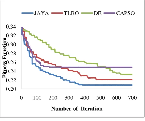
0.3381. Table-1 shows reactive power control variables (PV-bus voltages, shunt compensations and OLTCs) and all load bus voltages under base case condition. Threshold value of voltage stability margin selected asVSMth _{= 1.1027 pu.Initially, 100} populations of each control variable have been generated randomly using excel software according distribution characteristic of control variable. Maximum numbers of iteration is taken as 700 and terminated after 392 iterations. Table-2 shows the comparison of each algorithm to find the best optimal control variable settings with and without optimization using Jaya, TLBO, DE and CAPSO [25, 26] techniques.Table-3 shows the comparison of reactive reserves at different generator bus (bus nos. 1st, 2nd & 3rd)using Jaya, TLBO, DE and CAPSO techniques.Table-4shows the comparison of Jaya with TLBO, DE and CAPSO techniques based on arithmetic mean value, standard deviation, best value, worst value, frequency of convergence, standard error, length of confidence interval and confidence interval of fitness function [27]. Fig. 1 shows a plot for comparison of the convergence of fitness function with respect to number of iteration for Jaya, TLBO, DE and CAPSO techniques. Static voltage stability limit of the system is obtained using Jaya, TLBO, DE and CAPSO techniques are 5.3533pu, 5.2677pu,5.2164pu and 5.1308pu respectively. Voltage stability margin obtained at the end of optimization processes namely; Jaya, TLBO, DE and CAPSO techniques are 45.64%, 43.31%, 41.91% and 39.58% respectively. It is observed that Jaya gives much better global optimal results than TLBO, DE and CAPSO techniques.

Table-1. Load flow solution for 14-bus test system under

stressed condition.

Total load(𝑺𝒅) = 𝟑. 𝟔𝟕𝟓𝟖 𝒑𝒖, Static voltage stability

limit = 𝟒. 𝟔𝟖𝟓𝟖 𝒑𝒖

Fig. 1. Plot of convergence of fitness function with respect to number of iteration using Jaya, TLBO, DE and CAPSO techniques for IEEE 14-bus system.

IEEE 30-Bus System

The 30-bus [28] system consists of 6 generators, 24 load buses & 41 transmission lines. This system has 12 reactive power control variables; which are 6 generators (bus no. 1st, 2nd, 5th, 8th, 11th& 13th), and 4 OLTC (line number 11th, 12th, 15th& 36th) and 2 shunt compensations are connected at buses 10th and 24th, The limits of generators bus voltages and OLTCs have been assumed as 0.95pu to 1.15pu, and 0.90 to 1.10 respectively. Shunt compensations limit (lower and upper) of bus no. 10th, 0.00pu to 0.19pu and bus no. 24th, 0.00pu to 0.04pu [28] respectively. Reactive power limits (minimum and maximum) of generating bus no. 1st lying between −0.2000pu to 1.5000pu, bus no. 2nd lying between −0.2000pu to 0.6000pu, bus no. 5th lying between −0.1500pu to 0.6250pu, bus no. 8th lying between −0.1500pu to 0.5000pu, bus no. 11th lying between −0.1500pu to 0.4000pu, bus no. 13th lying between −0.1500pu to 0.4500pu [28]. The desired range of load bus voltage is 0.95pu to 1.05pu. The total base case active and reactive power demand on the system are 4.2626pu & 1.9222 pu, and fitness function F = 2.2925. Table-5 shows reactive power control variables (PV-bus voltages, shunt compensations and OLTCs) and all load bus voltages under base case condition. Threshold value of voltage stability margin selected as VSMth _{= 1.4028 pu.Initially, 50 populations of} each control variable have been generated randomly using excel software according distribution characteristic of control variable. Maximum numbers of generation is taken as 700 and terminated after 548 generations that are no improvement in fitness function. Table-6 shows the comparison of each

0.20 0.22 0.24 0.26 0.28 0.30 0.32 0.34

0 100 200 300 400 500 600 700

F

it

nes

s

F

un

ct

io

n

Number of Iteration

JAYA TLBO DE CAPSO

S. No

Control variables

Control variables Magnitude

(pu)

Load bus voltages

Load bus voltage Magnitude

(pu)

1 V1 1.0812 V4 0.8248

2 V2 1.0485 V5 0.8618

3 V3 1.0739 V6 0.9522

4 BSH4 0.0015 V7 0.8618

5 BSH12 0.0057 V8 0.9696

6 TAP4 1.0657 V9 0.8291

7 TAP10 1.0673 V10 0.8126

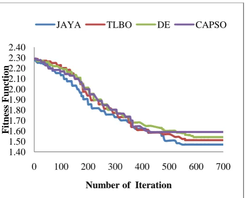
algorithm to find the best optimal control variable settings with and without optimization using Jaya, TLBO, DE and CAPSO techniques. . Table-7shows the comparison of reactive reserves at different generator bus (bus nos. 1st, 2nd, 5th, 8th, 11th& 13th)using Jaya, TLBO, DE and CAPSO techniques.Table-8shows the comparison of Jaya with TLBO, DE and CAPSO techniques based on arithmetic mean value, standard deviation, best value, worst value, frequency of convergence, standard error, length of confidence interval and confidence interval of objective function [27].Fig. 2 shows a plot for comparison of the convergence of fitness function with respect to number of iteration for Jaya, TLBO, DE and CAPSO techniques. Static voltage stability limit of the system is obtained using Jaya, TLBO, DE and CAPSO techniques are 7.4195pu, 7.1893pu,7.0185pu and 6.8948pu respectively. Voltage stability margin obtained at the end of optimization processes namely; Jaya, TLBO, DE and CAPSO techniques are 58.67%, 53.75%, 50.09% and 47.45% respectively. It is observed that Jaya gives much better global optimal results than TLBO, DE and CAPSO techniques.

Fig. 2. Plot of convergence of fitness function with respect to number of iteration using Jaya, TLBO, DE and CAPSO techniques for IEEE 30-bus system.

4. Conclusion

A methodology has been presented for the management of reactive power reserves in order to maintain voltage profile as well as voltage stability margin by using Jaya algorithm. These objectives are achieved by the rescheduling of the reactive control variables such as; PV-bus magnitude, OLTC and static VAR compensations. Jaya optimization

algorithm is based on the concept that the result obtained for a given problem should avoid the worst result and travel towards the best result. This algorithm requires only the common control parameters and does not require any algorithm-specific control parameters. This optimization algorithm is an efficient optimization method for large scale non-linear optimization problems for finding the global optimal solutions. Performance of the developed algorithm has been compared based on mean value, median value, mean deviation, variance, standard deviation, best value, worst value, frequency of convergence, standard error, length of confidence interval, confidence interval, class interval & proportionate frequencies of fitness function, with TLBO, DE and CAPSO techniques. It is observed that Jaya algorithm performs much better result than TLBO, DE and CAPSO techniques for IEEE 14-bus and 30-bus system.

References

[1] P. Kundur, ‘Power system stability and control ‘TMH, Edition, 1994.

[2] A. Tiranuchit and R.J. Thomas, ‘A posturing strategy against voltage instabilities in electric power systems’ IEEE Trans. on PS, 1988,Vol.3 , No.1, pp.81-93.

[3] M.M. Begovic and A.G. Phadke, ‘Control of voltage stability using sensitivity analysis ‘ IEEE Trans. on PS,

1992, Vol.7 , No.1 , pp. 114-123.

[4] A.M. Chebbo, M.R. Irving, and M.J.H. Sterling, ‘Reactive

power dispatch incorporating voltage stability’ Proc. IEEE Part-C, 1992, Vol.139, No.3, pp.253-260.

[5] V. Ajjarapu, P.L. Lau and S. Battula, ‘An optimal reactive power planning strategy against voltage collapse ’ IEEE Trans on PS, 1994, Vol.9, No.2, pp.906-917.

[6] Bansilal, D. Thukaram, and K. Parthsarthy, ‘optimal reactive power dispatch algorithm for voltage stability improvement’

Int. J. of Electrical Power and Energy systems, Vol.18, No.7, 1996 pp.461-468.

[7] P. Kessel and H. Glavitsch, ‘Estimating the voltage stability of power systems’ IEEE Trans. on PWRD, Vol.1, No.3, pp. 346-354.

[8] L.D. Arya, S.C. Choube and D.P. Kothari, ‘Reactive power

optimization using static voltage stability index’,‘Int. J. of Elect. Power components and systems’ Vol.29, March 2001, pp. 615-628.

[9] L.D. Arya, D.K. Sakravdia and D.P. Kothari, ‘corrective rescheduling for static voltage stability control’ Int. J. of Elec. Power and Energy systems, Vol.27, Jan.2005, pp.3-12. [10] V.S. Pande, L.D. Arya and S.C. Choube, ‘Artificial neural

network based reactive reserve management for voltage stability enhancement’ Proc. Int. Conf. on Power systems, Kathmandu, Nepal, Dec.3-6, 2004.

[11] L.S. Titare and L.D. Arya, ‘An approach to mitigate voltage collapse accounting uncertainties using improved particle swarm optimization’ Applied soft Computing Journal, Vol.19, No.4, sept.2009, pp.1197-1207.

[12] R. Taghavi, A.R. Seifi and M.N. Pourahmadi, ‘Fuzzy reactive power optimization in hybrid power systems’ Int. J Electrical power Energy systems, Vol.42, No.1, 2012, pp 375-383.

[13] A.H. Khazali and M. Kalantar, ‘optimal reactive power dispatch based on harmony search algorithm’ Int. J Electrical Power Energy Systems, Vol.33, No.3, 2011, pp.684-692.

[14] D. Devraj and J.P. Roselyn, ‘Genetic algorithm based reactive power dispatch for voltage stability improvement’ Int. J. Electrical power Energy system. Vol.32, No.10, 2010, pp.1151-1156.

1.40 1.50 1.60 1.70 1.80 1.90 2.00 2.10 2.20 2.30 2.40

0 100 200 300 400 500 600 700

F

it

nes

s

F

un

ct

io

n

Number of Iteration

[15] O.A. Mousavi, M. Bozorg and R. Cherkaowi, ‘Preventive

reactive power management for improving voltage stability margin’ Electric Power system Research, Vol.96, 2013, pp 36-46.

[16] H. Singh and L. Shrivastava , ‘Modified differential evolution algorithm for multi objective VAR management’

Int. J. of Electrical Power Energy systems, Vol.55, 2014 , pp. 731-740.

[17] L.S. Titare, P. Singh, L.D. Arya and S.C. Choube, ‘Optimal reactive power rescheduling based EPSDE algorithm to enhance static voltage stability’ Int. J. of Electrical Power and Energy systems, Vol.63, 2014, pp. 588-599

[18] S. Fang, H. Cheng, G. Xu, Q. Zhou, H. He and P. Zeng,

‘Stochastic reactive power dispatch considering voltage areas’ Int. Trans. on Electrical Energy system , Vol.27, No.3, March 2017, Doi 10.10.02/etep.2269

[19] B. Bhattacharya and S. Raj, ‘Differential evolution technique for the optimization of reactive power reserves’ Journal of circuits systems and computers (world’s scientific), Vol.26, No.10, October 2017, p.1750155

[20] Q. Sun, H. Cheng and Y. Song, ‘Bi-objective reactive power

reserve optimization to co- ordinate long and short term voltage stability’ IEEE Access, Date of publication 9, May 2017, DOI : 10.1109/ ACCESS. 2017.2701826

[21] S. Fang, H. Cheng, Y. Song, Z. Ma, Z. Zhu, P. Zeng and L. Yao, ‘Interval optimal reactive power dispatch considering generator rescheduling.’ IET Generation, Transmission and distribution , Vol.10, No.8, May 2016, pp. 1833-1841

[22] D.G. Rojar, J.L. Lezma and W. Villa, ‘Meta heuristic Techniques Applied to the optimal reactive power dispatch :

a review IEEE Latin America Transactions, Vol.14, No.5, May 2016, pp. 2253-2263

[23] R. Venkata Rao, ‘Jaya ; A simple and new optimization algorithm for solving constraints and un- constrained optimization problems’ International Journal of Industrial Engineering Computations, Vol.7, No.1, 2016, pp. 19-34. [24] R.V.Rao, V.J.Savsani and D.P. Vakharia, ‘

Teaching-learning-based optimization: An optimization method for continuous non-linear large scale problems’, Information Sciences, 2012, Vol. 183, No.1, pp. 1-15.

[25] R.Storn and K.Price,‘Differential evolution – a simple and efficient heuristic for global optimization over continuous spaces’ Journal Global Optimization, Vol. 11, No. 4, December 1997, pp. 341-359.

[26] G.J. Vlachogiannis and K.Y. Lee, ‘A comparative study on particle swarm optimization for optimal steady state performance of power systems’ IEEE Transactions on Power

Systems, Vol. 21, No. 4, 2006, pp. 1318-1328.

[27] Kreyszig, E.W., ‘Advance engineering mathematics’ John Wiley & Sons, Inc.; 2001 (Book).

[28] L.D. Arya and A. Koshti, ‘Anticipatory load shedding for line overload alleviation using Teaching learning based optimization (TLBO)’s, International Journal of Electrical Power & Energy Systems, vol. 63, 2014, pp. 862-877.

Table-2. Reactive power control variables using Jaya, TLBO, DE and CAPSO algorithms for IEEE 14-bus system (𝑺𝒅𝒕) = 𝟑. 𝟔𝟕𝟓𝟖𝒑𝒖.

Sr. No.

Reactive Control

Variables Base Case JAYA TLBO DE CAPSO

1 Tap4 1.0657 0.9317 0.9320 0.9326 0.9284

2 Tap10 1.0673 0.9266 0.9254 0.9258 0.9217

3 Qc4 0.0015 0.0508 0.0370 0.0447 0.0409

4 Qc12 0.0057 0.0473 0.0483 0.0357 0.0318

5 V1 1.0812 1.0788 1.0798 1.0797 1.0776

6 V2 1.0485 1.0428 1.0445 1.0457 1.0447

7 V3 1.0739 1.0693 1.0704 1.0716 1.0693

Table-3. Reactive power reserve at generator buses and fitness function using Jaya, TLBO, DE and CAPSO techniques for IEEE14-bus system (𝑺𝒅𝒕) = 𝟑. 𝟔𝟕𝟓𝟖𝒑𝒖.

Sr.

No. Methodology

Reactive Power Reserve (pu) _{Total Reactive Power}

Reserve (pu)

Fitness Function Qgk(res)1 Qgk(res)2 Qgk(res)3

1 JAYA 2.6991 0.8181 0.014 3.5312 0.2088

2 TLBO 2.7114 0.7916 0.0152 3.5183 0.221

3 DE 2.737 0.7646 0.012 3.5136 0.2326

4 CAPSO 2.7628 0.707 0.0319 3.5016 0.2489

Table -4. Comparison of Jaya with TLBO, DE and CAPSO techniques based on statistical interence for IEEE14-bus system.

Table-5 Load flow solution for 30-bus test system under stressed condition. Total load(𝑺𝒅) = 𝟒. 𝟔𝟕𝟓𝟗 𝒑𝒖, Static voltage stability limit = 𝟔. 𝟐𝟐𝟑𝟏 𝒑𝒖

O p tim iz a ti o n m eth o d s Ar ith m etic m ea n v a lu e o f th e o b je ctiv e fu n cti o n Medi a n v a lu e o f th e o b je ctiv e fu n ctio n Mea n d ev ia ti o n o f o b je ctiv e fu n ctio n Va ria n ce o f o b je ctiv e fu n ctio n S ta n d a rd d ev ia ti o n o f o b je ctiv e fu n ctio n Be st v a lu e o f o b je ctiv e fu n cti o n Wo rst v a lu e o f o b je ctiv e fu n ctio n Fre q u en cy o f co n v er g en ce Co n fid en ce lev el De te rm in ed v a lu e fo r th e E n g g . App li ca ti o n S ta n d a rd e rr o r o f th e m ea n o b je ctiv e fu n cti o n Co n fid en ce in te rv a l o f th e o b je ctiv e fu n cti o n Le n g th o f co n fi d en ce in te rv a l o f th e o b je ctiv e fu n ctio n (𝐹) (𝑚) (𝑑) (𝑠) (𝜎) (𝐹𝑏𝑒𝑠𝑡) (𝐹𝑤𝑜𝑟𝑠𝑡) (𝛾) (𝑐) (𝜀) (𝜇) (𝐿)

JAYA 0.2132 0.2115 2.00E-05 2.47E-05 0.0049 0.2088 0.2273 13 0.95 2.0452 0.0023 0.2109≤ 𝜇 ≤ 0.2155 0.0094

TLBO 0.2275 0.2255 4.00E-05 5.05E-05 0.0071 0.2210 0.2480 11 0.95 2.0452 0.0032 0.2243≤ 𝜇 ≤0.2307 0.0131

DE 0.2430 0.2421 1.50E-05 8.03E-05 0.0089 0.2326 0.2662 10 0.95 2.0452 0.0041 0.2389≤ 𝜇 ≤0.2471 0.0167

CAPSO 0.2669 0.2653 1.50E-05 1.77E-04 0.0133 0.2489 0.2951 10 0.95 2.0452 0.0061 0.2608≤ 𝜇 ≤0.2730 0.0249

S. No Control variables

Control variables magnitude(pu)

Load bus voltages

Load bus voltage magnitude(pu)

1 V1 1.0842 V3 1.0231

2 V2 1.0476 V4 1.0105

3 V5 1.0112 V6 1.0052

4 V8 1.0262 V7 0.9902

5 V11 1.0845 V9 0.9400

6 V13 1.0928 V10 0.8948

7 BSH10 0.0106 V12 0.9516

8 BSH24 0.0040 V14 0.9135

9 TAP11 1.0686 V15 0.8996

10 TAP12 1.0693 V16 0.9110

11 TAP15 1.0563 V17 0.8873

12 TAP36 0.9215 V18 0.8686

V19 0.8578

V20 0.8651

V21 0.8674

V22 0.8693

V23 0.8703

V24 0.8511

V25 0.8593

V26 0.8379

V27 0.8749

V28 0.9981

V29 0.8311

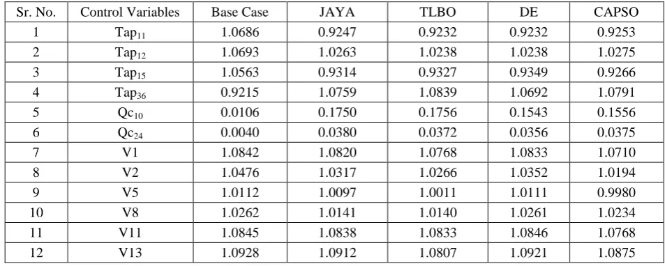
Table-6. Reactive power control variables using Jaya, TLBO, DE and CAPSO algorithms for IEEE 30-bus system (𝑺𝒅𝒕) = 𝟒. 𝟔𝟕𝟓𝟗𝒑𝒖.

Sr. No. Control Variables Base Case JAYA TLBO DE CAPSO

1 Tap11 1.0686 0.9247 0.9232 0.9232 0.9253

2 Tap12 1.0693 1.0263 1.0238 1.0238 1.0275

3 Tap15 1.0563 0.9314 0.9327 0.9349 0.9266

4 Tap36 0.9215 1.0759 1.0839 1.0692 1.0791

5 Qc10 0.0106 0.1750 0.1756 0.1543 0.1556

6 Qc24 0.0040 0.0380 0.0372 0.0356 0.0375

7 V1 1.0842 1.0820 1.0768 1.0833 1.0710

8 V2 1.0476 1.0317 1.0266 1.0352 1.0194

9 V5 1.0112 1.0097 1.0011 1.0111 0.9980

10 V8 1.0262 1.0141 1.0140 1.0261 1.0234

11 V11 1.0845 1.0838 1.0833 1.0846 1.0768

12 V13 1.0928 1.0912 1.0807 1.0921 1.0875

Table-7. Reactive power reserve at generator buses and fitness function using Jaya, TLBO, DE and CAPSO techniques for IEEE 30-bus system (𝑺𝒅𝒕) = 𝟒. 𝟔𝟕𝟓𝟗𝒑𝒖..

Sr. No.

Methodolo gy

Reactive Power Reserve (pu) _Reactive Total

Power Reserve (pu)

Fitness Function

Qgk(res)1 Qgk(res)2 Qgk(res)5 Qgk(res)8 Qgk(res)11 Qgk(res)13

1 JAYA 0.9759 0.2228 0.0337 0.3076 0.0547 0.0313 1.6260 1.4692

2 TLBO 0.9908 0.2099 0.0804 0.2292 0.0441 0.0589 1.6133 1.5119

3 DE 1.0301 0.2027 0.0791 0.1897 0.0684 0.038 1.608 1.5409

4 CAPSO 0.9931 0.3677 0.0855 0.0303 0.0716 0.0397 1.5879 1.5897

5 Base Case 1.2278 0.2272 0.0729 0.0965 -0.0749 -0.2348 1.3147 2.2925

Table -8. Comparison of Jaya with TLBO, DE and CAPSO techniques based on statistical interence for IEEE 30-bus system.

O p tim iza ti o n m eth o d s Ar ith m etic m ea n v a lu e o f th e o b je ctiv e fu n ctio n Medi a n v a lu e o f th e o b je ctiv e fu n cti o n Mea n d ev ia ti o n o f o b je ctiv e fu n cti o n Va ria n ce o f o b je ctiv e fu n ctio n S ta n d a rd d ev ia ti o n o f o b je ctiv e fu n cti o n Be st v a lu e o f o b je ctiv e fu n cti o n Wo rst v a lu e o f o b je ctiv e fu n cti o n Fre q u en cy o f co n v er g en ce Co n fid en ce lev el De te rm in ed v a lu e fo r th e En g . App li ca tio n S ta n d a rd e rr o r o f th e m ea n o b je ctiv e fu n ctio n Co n fid en ce in te rv a l o f th e o b je ctiv e fu n ctio n Le n g th o f co n fi d en ce in te rv a l o f th e o b je ctiv e fu n cti o n (𝐹) (𝑚) (𝑑) (𝑠) (𝜎) (𝐹𝑏𝑒𝑠𝑡) (𝐹𝑤𝑜𝑟𝑠𝑡) (𝛾) (𝑐) (𝜀) (𝜇) (𝐿)

JAYA 1.4814 1.4787 2.00E-05 1.40E-04 0.0118 1.4692 1.5142 12 0.95 2.0452 0.0054 1.4760≤ 𝜇 ≤1.4868 0.0221

TLBO 1.5348 1.5298 4.50E-05 4.02E-04 0.0200 1.5119 1.5849 11 0.95 2.0452 0.0091 1.5257≤ 𝜇 ≤1.5439 0.0372

DE 1.5781 1.5751 5.00E-05 7.64E-04 0.0276 1.5409 1.6479 10 0.95 2.0452 0.0126 1.5655≤ 𝜇 ≤1.5907 0.0515