http://www.sciencepublishinggroup.com/j/ijsda doi: 10.11648/j.ijsd.20180401.12
ISSN: 2472-3487 (Print); ISSN: 2472-3509 (Online)
A New Class of Generalized Burr III Distribution for Lifetime
Data
Olobatuyi Kehinde, Asiribo Osebi, Dawodu Ganiyu
Department of Statistics, Federal University of Agriculture, Abeokuta, Nigeria
Email address:
To cite this article:
Olobatuyi Kehinde, Asiribo Osebi, Dawodu Ganiyu. A New Class of Generalized Burr III Distribution for Lifetime Data. International Journal of Statistical Distributions and Applications. Vol. 4, No. 1, 2018, pp. 6-21. doi: 10.11648/j.ijsd.20180401.12
Received: January 4, 2018; Accepted: February 24, 2018; Published: March 28, 2018
Abstract:
For the first time, the Generalized Gamma Burr III (GGBIII) is introduced as an important model for problems in several areas such as actuarial sciences, meteorology, economics, finance, environmental studies, reliability, and censored data in survival analysis. A review of some existing gamma families have been presented. It was found that the distributions cannot exhibit complicated shapes such as unimodal and modified unimodal shapes which are very common in medical field. The Generalized Gamma Burr III (GGBIII) distribution which includes the family of Zografos and Balakrishnan as special cases is proposed and studied. It is expressed as the linear combination of Burr III distribution and it has a tractable properties. Some mathematical properties of the new distribution including hazard, survival, reverse hazard rate function, moments, moments generating function, mean and median deviations, distribution of the order statistics are presented. Maximum likelihood estimation technique is used to estimate the model parameters and applications to real datasets in order to illustrate the usefulness of the model are presented. Examples and applications as well as comparisons of the GGBIII to the existing Gamma-G families are given.Keywords: Burr III Distribution, Generalized-Gamma Distribution, Censored Data, Maximum Likelihood Estimation
1. Introduction
It is known that the Burr III distribution is the third example of solutions of the differential equation defining the Burr system of distribution, [4]. This distribution has been used widely in numerous fields of sciences with different parameterizations using other names. For example, it is used as inverse Burr distribution in the actuarial literature III distribution in low-flow frequency analysis where the lower tail of a distribution is of interest.[13] and kappa distribution in the meteorological literature ([17], 18]). The Burr III distribution has been useful in financial literature, environmental studies, in survival and reliability theory, (such as: [1, 7, 10, 14, 19, 26, 27]). Recently, [25] proposed the use of the so-called extended Burr.
A system of distributions which contains the Burr XII (BXII) distribution as the most widely used of these distributions was introduced [4]. If a random variable has the BXII distribution, then has the scaled Burr III (BIII) distribution with cumulative distribution function (cdf) defined for 0 by ([2]).
; , , 1 , 0, (1)
where
β
>
0
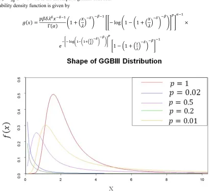
, 0 and 0, are shapes and scale parameters respectively. The probability density function corresponding to 1 is given by; , , 1 , (2)
The hazard and reverse hazard functions are given by:
; , ,
! "!"#$ %& '
"! (")"#
$ %&'"!(")
, (3)
and
* ; , , 1 (4)
. /0 ∗ 02 ∗ 0, 1 −0 , + < (5)
Where 2 5, 6 =7 8 7 97 :%; .
In this paper, a new class of Burr-type distribution called the Generalized Gamma-Burr III (GGBIII) distribution was presented and applied to some real-life situations.
Motivated by the various applications of Burr III distribution in finance and actuarial sciences, and economics, where distribution plays an important role in size distribution [2]. It is customary to develop models that take into consideration not only shape, and scale but also skewness, kurtosis and tail variations. An obvious reason for generalizing a standard distribution is to provide larger flexibility in modeling real data. It is well known in general that a generalized model is more flexible than the ordinary model and it is preferred by many data analysts in analyzing statistical data, [21]. The gamma distribution is the most effective model for analyzing skewed data [16].
In the last few years, several ways of generating new probability distributions from classic ones were developed and discussed. [12] Studied a distribution family that arises naturally from the distribution of order statistics. The beta-generated family proposed by [5] has been extensively used by many researchers in generalizing distribution. For any baseline continuous distribution with survival function 1 − and density , [28] defined the cumulative distribution function (cdf) and probability density function
(pdf) as follows
= =7 > ? CDE F @> A ,B@,
G H R, J > 0 (6)
and
K =7 > L− logO1 − PQ> , (7)
respectively. Also, an alternative gamma-generator was proposed [24] and definedthe cdf and pdf by
= = 1 −7 > ? CDE F R> A SBR,
G R H R, α > 0, (8)
and
K =7 > U− log V> , (9)
respectively. The exponentiated exponential (EE) distribution was generalized by [23] and further studied by [9] with cdf = O1 − A P>, where J > 0 and > 0 inserted into equation 8 to obtain and study the gamma exponentiated exponential (GEE) model. The statistical properties of the gamma – exponentiated Weibull distribution was presented [15]. The distribution with pdf K and cdf = for any baseline cdf define by [3] and H ℝ, (for J > 0) as follows
K =7 > YZL− logO1 − PQ >
O1 − P ⁄Y , (10)
= =7 > YZ?G CDEO F PR> A S Y⁄ BR, (11)
respectively, for J, \ > 0, where K =]^] , Γ J = ? R` >
G A SBR denotes the gamma function, and a @, J = ? R, >
G A SBR, denotes the incomplete gamma function. Towards the end, they obtained a natural extension for Dagum distribution, which they called the gamma-Dagum (GD) distribution.
A review of some existing gamma families have been presented, a different type of gamma generalized distribution was introduced [23], a Zografos and Balakrishnan-Dagum (ZB-D) was provided [23] which was modified by [3]. It was found that these distributions cannot exhibit complicated shapes such as unimodal and modified unimodal shapes which are very common in medical field.
In this paper, natural extension of Burr III distribution called the Generalized Gamma Burr III distribution was studied.
This paper is organized as follows. In section 2, some basic results, the generalized gamma-Burr III (GGBIII) distribution, series expansion and its sub-models, hazard, survival and reverse hazard functions and the quantile function are presented. The moments and moment generating function, mean and median deviations are given in section 3. Section 4 contains some additional useful results on the distribution of order statistics. In section 5, results on the estimation of the
parameters of the GGBIII distribution via the method of maximum likelihood are presented. Applications in different fields are presented in Section 6, followed by discussion in section 7 and conclusion in section 8.
2. The Generalized Gamma-G Family
The standard Gamma distribution of different kind is given by [8]
? R` b
G A S
c⁄Y
BR =7 b d⁄ Yd e c⁄ (12)
Then, we write equation 12 as
7 > YZ? Rd > A S c⁄Y
G BR (13)
This is the known gamma distribution when g = 1
Equation 13 has the parent distribution with the cdf given as follows
= =7 > YZ?L CDEO F PQ R> c
G A S Y⁄ BR (14)
Equation 14 is the generalization of Gamma-G family of [3] in equation 11 when g = 1 and also in equation 6 when g = \ = 1 [28].
gamma-G family of distributions when \ =1 is given by
= 7 > ?L CDEO F PQcR>
G A SBR (15)
Differentiating the equation 15 we obtain the pdf as follows
K 7 > LL3 logO1 3 PQdQ> A L CDEO F PQc]L CDEO F PQc
] (16)
K 7 > LL3 logO1 3 PQdQ> A L CDEO F PQcgL3 logO1 3 PQd l
F (17)
respectively, J, , , , g 0.
2.1.... Generalized Gamma Burr III Distribution
The new model is proposed by inserting scaled Burr III distribution into equation 15 , the cdf =^^mnnn of the Generalized Gamma-BIII distribution is obtained as follows:
= 7 > ?o CDEp $ % R>
& '
"! (")qr
c
G A SBR (18)
sto CDEp $ %&'"!(")qr c
,>u
7 > (19)
where a , J ? RG > A SBR is the incomplete gamma function. The probability density function is given by
K g Γ J $1 ( oo3 log p1 3 $1 ( qr
d r
> v
A o CDEp $ % & '
"! (")qr
c
w1 3 1 x (20)
Plots of the density function of the Generalized Gamma Burr III distribution for selected parameters values are given in figure 1. The plot indicates that the GGBIII distribution can be decreasing or right skewed.
2.2. Expansions of Density Functions
If a random variable has the GGBIII density, we write ~==2zzz J, , , , g . Let { = 1 + , and then using
the series representation, it gives
log 1 − { = |1 {~} `
}•
= |~ + 1{}% `
}•G
A U CDE € Vc
= | −1 -U− log 1 − { V d-ℎ! `
-•G
,
1
1 − { = | {‚ `
‚•G ,
U− log 1 − { Vd> = {d> ƒ| gJ − 1 „ `
…•G
{…p| {† ‡ + 2 `
†•G q
… ˆ,
and applying the result on the power series raised to a positive integer, with ‰†= ‡ + 2 , that is
p| ‰†{† `
†•G q
…
= | 5†,…{† `
†•G ,
where 5†,…= ‡‰G ∑ U„ ‹ + 1 − ‡V‰Œ•† Œ5† Œ,…, and 5G,…= ‰G…, [8], the GGBIII pdf can be written as
K^^mnnn =
d ! "!"#w %& '
"! x")"#
7 > {d> × ∑ ∑`…•G `†•G d>… 5†,…{…%†∑ −1- U CDE € V c• -! `
-•G ∑ {`‚•G ‚ (21)
= d! "!"#w % & '
"! x")"#
7 > × ∑ ∑…•G` †,•G` ∑-•G` ∑‚•G` d>… −1 - U CDE € V c•
-! 5†,…{d>%†%…%‚ (22)
= ∑ ∑ ∑ ∑ −1 - d> …
d ! "!"#w %& ' "! x")"# 7 > ` ‚•G ` -•G ` †•G `
…•G × U CDE € V
c•
-! 5†,…{d>%†%…%‚ (23)
= ∑ ∑ ∑ ∑ −1 - d> …
d ! "!"#w %& ' "! x")"# 7 > ` ‚•G ` -•G ` †•G `
…•G ×U CDE € V
c•
-! 5†,…Ž1 + •
d>% †% …% ‚%
(24)
= ∑ ∑ ∑ ∑ −1 - d>
… d ! "!"# 7 > ` ‚•G ` -•G ` †•G `
…•G × 5†,…Ž1 + •
d>%†%…%‚
U CDE € Vc•
-! (25)
= ∑ ∑ ∑ ∑ −1 - d>
… d
! d>%†%…%‚ "!"# 7 > d>%†%…%‚ ` ‚•G ` -•G ` †•G `
…•G 5†,… × Ž1 + •
d>%†%…%‚
U CDE € Vc•
-! (26)
= ∑ ∑ ∑ ∑ -!• d>
… d
! d>%†%…%‚ "!"# 7 > d>%†%…%‚ ` ‚•G ` -•G ` †•G `
…•G 5†,…× Ž1 + •
d>%†%…%‚
w− log $1 − 1 + (x
(27)
where ; , gJ + „ + ‡ + • , is the Burr III pdf with parameters , gJ + „ + ‡ + • and . Let ” = • „, ℎ, ‡, • H –%—˜
™š= • -! d>…
:›,œ
7 > d>%†%…%‚, (28)
K^^mnnn = ∑ ™š•ž š ; , gJ „ ‡ • , . (29)
2.3. Hazard and Reverse Hazard Functions
Let be a continuous random variable with distribution function , and probability density function (pdf) , then the hazard function, reverse hazard function are given by F ⁄O1 3 P. The hazard and reverse hazard function of the GGBIII distribution are
g 1
$1 3 1 ( v w3 log $1 3 1 (x
d>
v A o CDEp $ % "!
(")qr c
Γ J 3 a pw3 log w1 3 1 xx
d , Jq
and
*
g 3 31 1 3 3 31
t#"$#Ÿ &'"!(")u
vo CDEp $ % &'"!(")qr cZ"#
vA
3ƒ" ¡¢t#"$#Ÿ &'"!(")uˆ g
sto CDEo $ %&'"!(")rr c
,>u
(30)
respectively, for £ 0, £ 0, £ 0, J £ 0, g £ 0, and £ 0.
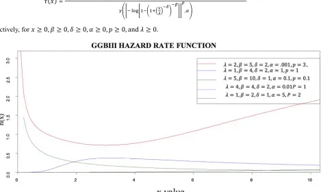
Figure 2. THE Plot of Hazard Rate Function of GGBIII.
The plots show various shapes including monotonically decreasing, monotonically increasing, and bathtub followed by upside down bathtub shapes for five combinations of values of the parameters. This very attractive flexibility makes the GGBIII hazard rate function useful and suitable for monotonic and non-monotone empirical hazard behaviors which are more likely to be encountered or observed in real life situations.
2.4. GGBIII Quantile Function
Let X be a random variable with distribution function F, and let ¤ ∈ 0, 1 . A value of x such that
¦ 4 § ¤ and ¦ § £ ¤ is called a
quantile of order ¤ for the distribution. Roughly speaking, a quantile of order ¤ is a value where the graph of the cumulative distribution function crosses (or jumps over) ¤.
The quantile function of GGBIII distribution is obtained by solving the equation
¤ = ¨•©• H ª: ≥ ¤˜, ¤ ∈ 0,1 ¬^^mnnnO dP = ¤, 0 < ¤ < 1.
¬^^mnnn ¤ = Ž 1 − A €# c⁄ ⁄
− 1• ⁄ (31)
then a {, J = ¤Γ J , where { = a ¤Γ J , J .
3. Moments, Moment Generating
Function, Mean and Median
Deviations
In this section, the moments, moment generating function, mean and median deviations for the GGBIII distribution were presented.
3.1. Moments and Moment Generating Function
As with any other distribution, many of the interesting characteristics and features of the GGBIII distribution can be studied through the moments. Let ∗= gJ + „ + ‡ + • , and /~ 2zzz , , ∗ . Then the +,- moment of the random variable / is
. /0 = ∗ 02 ∗+0, 1 −0 , + < (32)
So that the +,- raw moment is thus given by the following
. 0 = ∑ ™ š
š•ž ∗ 02 ∗+0, 1 −0 + < , (33)
The moment generating function of the BGBIII distribution is given by
-® @ = . A,® = . ¯1 + @ + ,® ° ±! +
,®²
—! + ⋯ ´, (34)
= |@+! .0 0 `
0•
,
then we have,
∑`0•G∑š•ž,0!µ™š ∗ 02 ∗+ +⁄ , 1 − +⁄ + < , (35)
3.2. Mean and Median Deviations
3.2.1. Mean Deviation
If X has the GGBIII distribution, we derive the mean deviation about the mean ¶ by
= ? | − ¶|G` K^¸ B = 2¶=^^mnnn ¶ − 2¶ + 2¹ ¶ , (36)
Where ¶ = . and ¹ ¶ = ?»` ∙ K^^mnnn B . Let ∗= gJ + „ + ‡ + • , then
¹ ¶ = ∑ ™š•ž š¹^^mnnn ∗, , ¶ (37) = ∑ ™š•ž š ∗ U2 ∗+ 1⁄ , 1 − 1⁄ − 2 @ ¶ ; ∗+ 1⁄ , 1 − 1⁄ V (38)
= 2 | ™š š•ž
∗ U2 ∗+ 1⁄ , 1 − 1⁄ V
¼ ½ ½ ½ ½
¾a pw−logw1 − 1 + ¶ xx d
, Jq
Γ J − 1
¿ À À À À Á
+2 ∑ ™š•ž š ∗ U2 ∗+ 1⁄ , 1 − 1⁄ − 2 @ ¶ ; ∗+ 1⁄ , 1 − 1⁄ V (39)
Where @ ¶ = 1 + » and 2 ; 5, 6 = ? @G : 1 − @ ; B@.
3.2.2. Median Deviation
If has the GGBIII distribution, then the median deviation about the median - is derived by
±= ? | − -|G` K^¸ B = 2¹ - − ¶, (40)
where ¹ - = ?Â` ∙ K^^mnnn B
- = ¬^^mnnn 0.5 = w 1 − A Ls"#G.Ã7 > ,> Q # c⁄ ⁄
− 1x ⁄ (41)
¹ - = | ™š¹mnnn ∗, , -š•ž
2 ∑ ™š•ž š ∗ U2 ∗+ 1⁄ , 1 − 1⁄ − 2 @ - ; ∗+ 1⁄ , 1 − 1⁄ V− ∑ ™š•ž š ∗ U2 ∗+ 1⁄ , 1 − 1⁄ V (43)
4. Order Statistics of Ggbiii Distribution
Definition: Let y , … , yÆ be a random sample from the GGBIII distribution with pdf f y defined over the interval −∞ to ∞. A rearrangement of the random sample into x , … , xÆ i.e. −∞ < x , x±, … xÆ< ∞ is known as the ordered transformation of the random sample and x , x±, … , xÆ are called ordered statistics.
Theorem: Let , ±, … , Ê be ordered statistics of a random sample y , … , yÆ from a GGBIII distribution with pdf K , the joint pdf is given as
, ±, . . , Ê = ©! K K ± … K Ê Ë+ − ∞ < < ±< ⋯ < Ê< ∞. The general formula for order statistics is given by
‚;Ê = Ê ‚ ! ‚Ê!Ì !U= V‚ U1 − = VÊ ‚, (44)
Again, using the binomial expansion to the second factor, it gives
‚;Ê = Ê ‚ ! ‚Ê!Ì !∑Ê ‚…•G −1 … Ê ‚… U= V‚%… , (45)
‚;Ê = Ê ‚ ! ‚Ê!Ì !∑Ê ‚…•G −1 … Ê ‚… w
s L CDEO F PQc,> 7 > x
‚%…
(46)
From [8]
a , J = | −1~ + J ~!} }%> `
}•Í
,
and if B}= −1 }ÎO ~ + J ~!P, then
‚;Ê = Ê ‚ ! ‚Ê!Ì !∑ Ê ‚…
œ
U7 > VÏŸœ"# ¯L− logO1 − PQ´ d > ‚%… Ê ‚
…•G × o∑
ЯL CDEO F PQc´Ð }%> }! `
}•G r
‚%…
(47)
‚;Ê = Ê ‚ ! ‚Ê!Ì !∑ Ê ‚…
œ
U7 > VÏŸœ"#OL− logO1 − PQ d
P> ‚%… × ∑ OL− logO1 −` PQdP}
}•G ,
Ê ‚
…•G (49)
‚;Ê = Ê ‚ ! ‚Ê!Ì !∑ ∑ Ê ‚…
œ]Ð,Ñ"ÏŸœ
U7 > VÏŸœ"# OL− logO1 − PQdP
> ‚%… %} `
}•G Ê ‚
…•G (50)
=Ê!dOL CDEO F PQPcZ"#Ê ‚ ! ‚Ò"L" ¡¢O#"Ó & PQc!7 > U F V"#l ∑ ∑ Ê ‚ … ` }•G Ê ‚ …•G
œ]Ô,ÏŸœ"#
U7 > VÏŸœ"# × OL− logO1 − PQ d
P> ‚%… %} (51)
= Ê ‚ ! ‚Ê! !∑ ∑ Ê ‚ … ` }•G Ê ‚ …•G
œ]Ô,ÏŸœ"#
U7 > VÏŸœ OL− logO1 − PQ d
Pd> ‚%… %} A L CDEO F PQcU1 − V (52)
= Ê ‚ ! ‚Ê! !∑ ∑ Ê ‚ … ` }•G Ê ‚ …•G
œ]Ô,ÏŸœ"#
U7 > VÏŸœ ×7O > ‚%… %} P7O > ‚%… %} PL− logO1 − PQ
d> ‚%… %}
× A L CDEO F PQc× U1 − V (53) That is,
‚,Ê = Ê ‚ ! ‚Ê! !∑ ∑Ê ‚…•G `}•G Ê ‚…
œ]Ô,ÏŸœ"#7 > ‚%… %}
U7 > VÏŸœ × ; J • + „ + ~, g, , , , (54)
where ; J • + „ + ~, g, , , is the GGBIII pdf with parameters , , , g and shape parameter J∗= J • + „ + ~.
= © − • ! • − 1 ! | |©! © − •„ `
}•G Ê ‚
…•G
−1 …BÕ,‚%… ΓO J • + „ + ~ P UΓ J V‚%…
g 1 +
w− log $1 − 1 + (x
d> ‚%… %}
A o CDEp $ % & '
"! (")qr
c
w1 − 1 + x (55)
5. Maximum Likelihood Estimation
The maximum likelihood estimation (MLE) is one of the most widely used estimation method for finding the unknown parameters. Consider a random sample , ±, … , Ê from the generalized gamma-Dagum distribution.
The likelihood function is given by
Ö , J, , , g =Og P Ê
UΓ J VÊ
∏ Ø ‚ Ž1 + Ï • w− log $1 − 1 + Ï (x d>
¯1 − O1 + ‚ P ´ × A
o CDEp $ %&Ï' "!(")qr c
Ù Ê
‚• (56)
where Ú = g, J, , , Û
Now, the log-likelihood function denoted by ℓ
ℓ = logUÖ Θ V
Ö \ = © logO P + © log g + © log + © log − © log Γ J − + 1 ∑ logÊ‚• ‚ − + 1 ∑ log 1 +Ê‚• Ï + gJ − 1 ∑ log ¯−log 1 − O1 +Ê‚• ‚ P ´ − ∑ log ¯1 − O1 +Ê‚•G ‚ P ´ − ∑ ¯−log 1 − O1 + ‚ P ´
d Ê
‚• (57)
The partial derivatives of ℓ with respect to the parameters are
ÞŒ Þ>= −©
7ß>
7 > + g ∑ log w− log $1 − 1 +Ê‚•G Ï (x (58)
à‹
à =©− | log $1 + ‚ ( Ê
‚•
− gJ − 1 | 1 +
‚ log 1 + ‚
$1 − 1 + ‚ ( log $1 − 1 + ‚ ( Ê
‚•G
−
∑ $ %&Ï' "!
(")CDE$ %&Ï' "!(
p $ %&Ï' "!(")q Ê
‚•G − g ∑
o CDEp $ % &Ï' "!(")qr c"#
$ %&Ï' "!(")CDE$ % &Ï' "!(
p $ %&Ï' "!(")q Ê
‚• (59)
à‹
à =©− © log − | log ‚+ + 1 | ‚ ‹ËK ‚ 1 + ‚ Ê
‚• Ê
‚•
+ gJ − 1 | 1 +
‚ ‚ log ‚
w1 − 1 + ‚ x $log $1 − 1 + ‚ (( Ê
‚•
−g ∑ o CDEp $ % &Ï
' "!
(")qr c"#
&Ï '
"!
$ %&Ï' "!(")CDE &Ï'
o $ %&Ï' "!(")r Ê
‚• + ∑
$ %&Ï' "!(") &Ï' "!CDE&Ï'
p $ %&Ï' "!(")q Ê
‚• (60)
à‹
à =© − + 1 | ‚
1 + ‚ + gJ − 1 |
‚ O1 +
‚ P
$1 − 1 + ‚ ( w−log $1 − 1 + ‚ (x Ê
‚• Ê
‚•
g ∑ o CDEp $ % &Ï
' "!
(")qr c"#
$ %&Ï' "!(") &Ï' "!!'
o $ %&Ï' "!(")r Ê
‚• − ∑ % Ï
"! ") &Ï ' "!!'
o $ %&Ï' "!(")r Ê
‚• (61)
ÞŒ Þd=
Ê
d+ J ∑ log w− log w1 − 1 +Ê‚•G Ï xx+ ∑ $log w1 − 1 + Ï x( d
log $log w1 − 1 + Ï x( Ê
‚• (62)
respectively. The MLE of the parameters , , , g, J will be obtained and they are denoted by á, á, ĝ, á, Jã. Asymptotic confidence intervals
The asymptotic confidence intervals for the parameters of the GGBIII distribution are presented. The expectations in the Fisher Information Matrix (FIM) will now be obtained numerically. The approximate 100 1 − ä % two-sided confidence intervals for , , , J, g. are given by:
á ± –Ê
±çz OΘèP, á ± –ʱçz OΘèP, á ± –ʱçz OΘèP, Jã ± –±Êçz>>OΘèP, ĝ ± –ʱçzddOΘèP,
Under the usual regularity conditions, the well-known asymptotic properties of the maximum likelihood method
ensure that √© OÚê − ΘPÊ → ì 0, Σ] î , where the Σî= Uz Θ V is the asymptotic variance-covariance matrix and
z Θ =
ï ð ð ñ
ò>> ò > ò > ò> ò ò ò>
ò> ò>d
ò ò ò d
ò ò òd
ò> òd> ò òd ò ò òd
òd òd òddó
ô ô õ
We can use the likelihood ratio (LR) test to compare the fit of the GD distribution with its sub-models for a given data set. The LR test rejects the null hypothesis if ö > ÷ø± where ÷ø±denote the upper 100% point of the ÷± distribution with 2 degrees of freedom.
6. Applications
In this section, we present applications of the proposed
GGBIII distribution and compare it to the existing Gamma-G families in real data sets to illustrate its potentiality and robustness. The maximum likelihood estimates (MLEs) of the GGBIII parameters J, , , and g are computed by maximizing the objective function via the sub-routine NLMIXED in SAS. The estimated values of the parameters (standard error in parenthesis), -2log-likelihood statistic, Akaike Information Criterion, Bayesian Information Criterion, and Corrected Akaike Information Criterion are presented. Also, presented are values of Likelihood Ratio test, Kolmogorov-Smirnov, Cramer-Von Mises, Anderson-Darling statistic for hypothesis test which were obtained using a package fitdistrplus in R. In order to compare the models above with the proposed model, we applied formal goodness-of-fit tests to verify which distribution fits better to the real data sets. Here, we consider the Anderson-Darling ù , CramÁr-von Mises û and Kolmogorov-Smirnov statistics üý. In general, the distribution which has the smallest values of these statistics is the better fit for the data.
Table 1. Descriptive Statistics for the Datasets Used.
Data N Mean Median Mode SD Var Skewness Kurtosis Min Max
Myelo 33 40.88 22.00 4.00 46.70 2181.17 1.22 0.35 1 156
Aircon 188 92.07 54.00 14.00 107.92 11645.93 2.16 5.19 1 603
Airc 30 85.93 22.00 11.00 165.72 27463.58 4.06 18.83 1 877
Comp 50 3.34 1.41 4.181 17.48 1.46 1.33 0.04 15.04
Cancer 1207 46.96 42.97 18.67 29.63 878.46 0.63 - 0.24 2.63 133.80
6.1. Acute Myelogeneous Leukemia
The first real data set represents the survival times, in weeks, of 33 patients suffering from acute Myelogeneous Leukemia. These data have been analyzed by [6]. The data are: 65, 156, 100, 134, 16, 108, 121, 4, 39, 143, 56, 26, 22, 1, 1, 5, 65, 56, 65, 17, 7, 16, 22, 3, 4, 2, 3, 8, 4, 3, 30, 4, 43. For these data, we shall compare the proposed GGBIII distribution to Gamma Dagum (GD) ([3]), alternative Gamma Dagum (GD) ([11]), Zografos and Balakrishnan Dagum (ZB-D) ([28]).
=
ï ð
ñ0.004620
9593 0.0106779546 30.000327988 0.0106779546 0.0246161742 30.000759203
30.00032799 0.0002427039 12.260556843
30.000759203 0.0004654929 25.152922308
0.0000231093 30.000057774 31.551993882
2.427039e3 04 12.26055684 4.654929e3 04 25.15292231 35.77747e3 05
1.899781e3 07 1.445071e3 02
31.55199388 0.014450710 1166.046687ó
ô õ
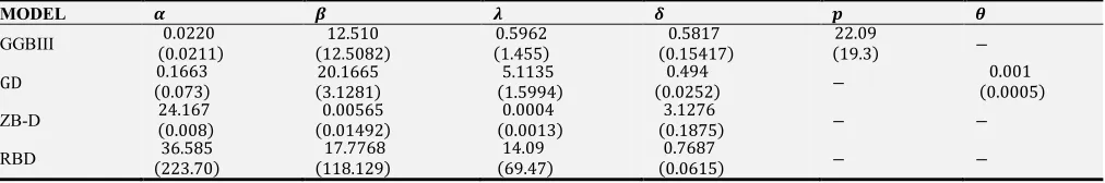
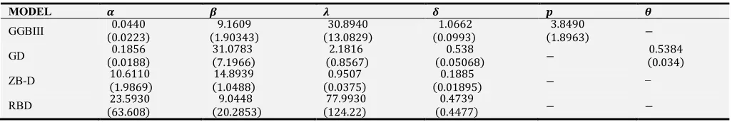
Table 1 lists the MLEs of the model parameters for GGBIII, GD, RBD, ZBD models, the corresponding standard errors (given in parentheses) and the statistics ù, KS and û.
These results show that the GGBIII distribution has the lowest ù∗, KS and û∗. values among all the fitted models, and so it could be chosen as the best model.
Figure 3. The histogram of the acute myelogeneous data and the estimated fitted distributions.
Figure 4. The ECF of the acute myelogeneous data and the estimated fitted distributions.
Table 2. The Maximum Likelihood Estimation of the Generalized Gamma Burr III distribution for the Acute Myelogeneous Data.
MODEL
GGBIII 0.02200.0211 12.508212.510 0.51.455962 0.15410.58177 22.019.39 3
GD 0.16630.0
73
20.1665
3.1281 1.5 5.1135 994
0.494
0.0252 3 0.00050.001
ZB-D 0.00824.167 0.005650.014
92
0.0004
0.0013 0.183.127765 3 3
RBD 223.36.58570 118.1217.77689 614.09.497 0.06150.7687 3 3
Table 3. THE AIC, AICc and BIC for the Distributions.
MODEL 3 3
GGBIII 299.2 309.2 311.4 316.7
GD 303.6 313.6 315.8 321.1
ZB-D 308.7 316.7 318.2 322.7
RBD 307.4 315.4 316.8 321.4
Table 4. Likelihood Ratio Test Statistic.
MODEL ! "#$ % ! !&
GGBIII vs GD 'G: =()‡ ': ==2zzz 4.4
GGBIII vs RBD 'G: ª2()‡ ': ==2zzz 8.2
Figure 5. The P-P of the acute myelogeneous data and the estimated fitted distributions.
6.2. The Air Conditioning System Data
The second example consists of the number of successive failures for the Air conditioning system of each member in a fleet of 13 Boeing 720 jet airplanes ([22]).
Table 5. Air conditioning system data.
194 413 90 74 55 23 97 50 359 50 130 487 57 102 15 14 10 57 320 261 51 44 9 254 493 33 18 209 41 58 60 48 56 87 11 102 12 5 14 14 29 37 186 29 104 7 4 72 270 283 7 61 100 61 502 220 120 141 22 603 35 98 54 100 11 181 65 49 12 239 14 18 39 3 12 5 32 9 438 43 134 184 20 386 182 71 80 188 230 152 5 36 79 59 33 246 1 79 3 27 201 84 27 156 21 16 88 130 14 118 44 15 42 106 46 230 26 59 153 104 20 206 5 66 34 29 26 35 5 82 31 118 326 12 54 36 34 18 25 120 31 22 18 216 139 67 310 3 46 210 57 76 14 111 97 62 39 30 7 44 11 63 23 22 23 14 18 13 34 16 18 130 90 163 208 1 24 70 16 101 52 20895 62 11 191 14 71
The asymptotic covariance matrix of the MLEs of the GGBIII model parameters, which is the inverse of the observed Fisher information matrix zÊ OΔèP is given by:
=
ï ð
ñ0.554348211 0.3
73214023 30.0199769930
0.373214023 0.232368967 30.015293134
30.01997699
0.008048857
0.272517683
30.01529313
0.004651359
0.151946115
0.00045638670
30.0007273570
30.0848136726
0.0080488570 0.272517683
0.0046513590 0.151946115
30.000727357
6.844605e3 05
1.974827e3 03
30.08481367
0.001974827
0.051271694ó
ô õ
Table 6. The Maximum Likelihood Estimation of the Generalized Gamma Burr III Distribution for the Air Conditioning System Data.
MODEL
GGBIII 0.04400.0223 1.9.1609
90343
30.8940
13.0829
1.0662
0.0993
3.8490
1.8963 3
GD 0.18560.0188 31.0783
7.1966
2.1816
0.8567
0.538
0.05068 3 0.034 0.5384
ZB-D 1.10.6110
9869
14.8939
1.0488 0.0.03950775
0.1885
0.01895 3 −
Figure 6. The histogram of the Air conditioning data and the estimated fitted distributions.
Figure 7. The cumulative function of the Air conditioning data and the estimated fitted distributions.
Figure 8. The P-P plot of the Air conditioning data and the estimated fitted distributions.
Table 7. The −2Ö, AIC, AICc and BIC of the Distributions.
MODEL 3
GGBIII 2062.9 2072.9 2073.3 2089.1
GD 2065.1 2075.1 2075.4 2091.2
ZB-D 2084.7 2092.7 2092.9 2105.7
RBD 2066.9 2074.9 2075.1 2087.8
Table 8. The Likelihood Ratio Test Statistic.
MODEL +,- . / / 01.2. /. 3
GGBIII vs GD 'G: =()‡ ': ==2zzz 2.2
GGBIII vs RBD 'G: =()‡ ': ==2zzz 4.0
GGBIII vs ZB-D 'G:=()‡ ':==2zzz 21.8
Table 9. Goodness of Fit Statistic for Air Conditioning System Data.
MODEL 9! 45%6 5 7 8$ % ! !& :8; 5 8 ;%5<!8=$ % ! !& $6!58 ?> <6 = 5 ?$ % ! !&
GGBIII 0.03536 0.26363 0.03815
GD 0.04063 0.28902 0.04296
RB-D 0.03807 0.30803 0.04151
ZBD 0.13285 1.08089 0.05574
6.3. Failure Times of 50 Components (Per 1000 Hours)
Real dataset was used to show that the GGBIII distribution is a better model when compared to GD, RBD, and ZBD distribution. The dataset taken from ([20]) represents the failure times of 50 components (per 1000h):
Table 10. The Failure Time of 50 Components Data.
0.036, 0.058, 0.061, 0.074, 0.078, 0.086, 0.102, 0.103, 0.114, 0.116, 0.148, 0.183, 0.192, 0.254, 0.262, 0.379, 0.381, 0.538, 0.570, 0.574, 0.590, 0.618, 0.645, 0.961, 1.228, 1.600, 2.006, 2.054, 2.804, 3.058, 3.076, 3.147, 3.625, 3.704, 3.931, 4.073, 4.393, 4.534, 4.893, 6.274, 6.816,7.896, 7.904, 8.022, 9.337, 10.940, 11.020, 13.880, 14.730, 15.080.
=
ï ð
ñ1.02864
7e3 01 8.474526e3 03 0.0140114350
8.474526e3 03 3.678572e3 03 0.0051354478
1.401144e3 02 9.055202e3 04
1.259102e 01
5.135448e3 03
8.182118e3 05
1.678922e 00
0.0049282620
0.0001009937
2.7315266258
9.055202e3 04 12.591021456
8.182118e3 05 1.678922408
1.009937e3 04 9.044504e3 08
1.921215e3 03
2.731526626
0.001921215
43.107069967ó
ô õ
Table 11. The Maximum Likelihood Estimation of the Parameters for Failure Time of Components Per Hour.
MODEL
GGBIII 0.080.069
7
4.079
2.932
0.358
0.752
0.563
0.179
5.618
3.076 3
GD 0.5600.852 3.838 3.
722
1.681
1.299
0.417
0.236 3 0.1040.198
RB-D 6.17.77560 2.4.27794 0 12.8.018910 0.5620.483 3 3
ZB-D 0.00.01176 5.4240.004 70.01.930
9
1.331
0.004 3 3
Table 12. The 32Ö, AIC and BIC of the Distributions for Failure Time of Components per Hour.
MODEL 3 " =3"!@ <! ; :A4 BA4
GGBIII 198.4 208.4 217.9
GD 205.9 215.9 255.4
ZB-D 207.9 215.9 223.6
RBD 205.5 213.5 221.2
Table 13. The Likelihood Ratio Test Statistic.
MODEL ! "#$ % ! !&
GGBIII vs GD 'G: =()‡ ': ==2zzz 7.5
GGBIII vs RBD 'G: =()‡ ': ==2zzz 7.1
GGBIII vs ZB-D 'G: =()‡ ': ==2zzz 9.5
Table 14. Goodness of Fit Statistic for Components Data.
MODEL 45%6 537 8
9! $ % ! !&
:8; 5 83;%5<!8= $ % ! !&
> <6 = 5 ? $6!58 ?$ % ! !&
GGBIII 0.12097 0.75666 0.10417
GD 0.16636 1.02411 0.12379
RB-D 0.17121 1.05099 0.12923
ZB-D 0.14148 0.92404 0.11922
Figure 9. The histogram of the Air conditioning data and the estimated fitted distributions.
Figure 11. The P-P plot of the Air conditioning data and the estimated fitted distributions.
Figure 12. The Esf of the Air conditioning data and the estimated fitted distributions.
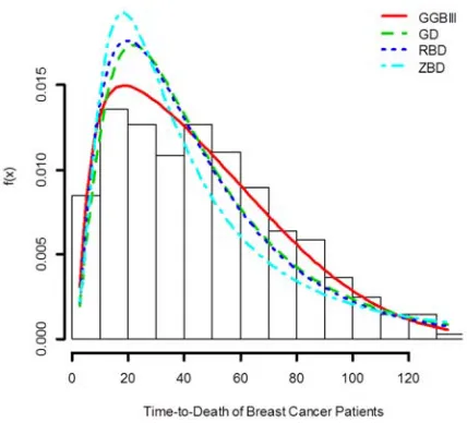
6.4. Breast Cancer Survival Data
The application of the GGBII distribution to a breast cancer data was developed. The study cohort comprises 1207 patients with cancer treated by mastectomy. Patient data were obtained from the database of SPSS software. The data consist of number of months after mastectomy. Uncensored observations correspond to patients having death time computed. Censored
observations correspond to patients who were not observed to have died at the time the data were collected. The numbers of censored and uncensored observations are 1135 and 72, respectively, of the total of 1207 patients.
Figure 13. The histogram of the Breast cancer data and the estimated fitted distributions.
Figure 14. The Ecf of the Breast cancer data and the estimated fitted distributions.
The asymptotic covariance matrix of the MLEs of the GGBIII model parameters, which is the inverse of the observed Fisher information matrix zÊ OþèP is given by:
=
ï ð ñ0.02
7479129 0.0070660643 31.08292e3 03
0.007066064 0.0017795919 32.87801e3 04
30.0010829
0.001209875
0.093244254
30.000287801
0.0002736553
0.0193527713
3.732178e3 05
31.02690e3 04
1.099804e3 01
1.209875e3 03 0.0932442544
2.736553e3 04 0.0193527713
31.02690e3 04
1.710644e3 05
8.351013e3 04
0.1099804175
0.0008351013 0.0354401755ó
ô õ
0 5 10 15
0
.0
0
.2
0
.4
0
.6
0
.8
1
.0
Empirical survival function for FAILURE MACHINE data
Faliure Machine data
S
(t
)
Table 15. The Maximum Likelihood Estimation of the Parameters for Time-to-Death of the Breast Cancer Patients.
MODEL
GGBIII 0.25230.0363 10.1882.33347 0.36550.8490 0.640.045690 6.00.501770
9 −
GD 0.4410.03637 32.142.10591
9
1.3056 0.0925
0.5710
0.0233 − 0.000.03097
ZB-D 0.10.00527549 12.00.00983
97
80.292
0.01515 1.450.004590
RBD 14.311. 930
7487
5.5995
3.5564 13970.11620.23
0.9590
0.2591
Table 16. THE −2Ö, AIC, AICC AND BIC OF THE MODELS.
MODEL − " =−"!@ <! ; :A4 BA4
GGBIII 11332.4 11342.4 11367.9
GD 11439.7 11449.7 11475.2
ZB-D 11640.8 11650.8 11671.2
RBD 11454.4 11464.4 11484.8
Table 17. The Likelihood Ratio Test Statistic.
ODEL ! "#$ % ! !&
GGBIII vs. GD 'G: =()‡ ': ==2zzz 107.33
GGBIII vs. RBD 'G: =()‡ ': ==2zzz 122.01
GGBIII vs. ZB-D 'G: =()‡ ': ==2zzz 308.44
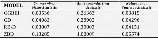
Table 18. Goodness of Fit Statistic for Breast Cancer Data.
MODEL 9! 45%6 5 7 8$ % ! !& :8; 5 8 ;%5<!8=$ % ! !& $6!58 ?> <6 = 5 ?$ % ! !&
GGBIII 0.44366 2.18208 0.03976
GD 3.05180 14.78988 0.09135
RB-D 1.86892 10.95541 0.07256
ZB-D 3.86745 23.31508 0.10140
Figure 15. The P-P plot of the Breast cancer data and the estimated fitted distributions.
Summary of the Findings
A new five-parameter distribution named the Generalized Gamma Burr III distribution has been introduced. It is the generalization of the Burr III distribution.
The proposed distribution has the ability to capture monotonically increasing, decreasing and unimodal hazard
rates.
It also reveals that GGBIII distribution has widened the scope of gamma-G family into the area of survival analysis and it has been found amenable in the medical area.
Finally, it was shown that the proposed distribution gave the best fit for five well-known data sets (when compared to other distributions including one having five parameters).
7. Discussion
A new class of generalized Burr III distribution called the generalized gamma-Burr III distribution is proposed and studied. The idea is to combine two components in a serial system, so that the hazard function is either increasing or more importantly bathtub shaped and unimodal shaped. The GGBIII distribution has the family of Zografos and Balakrishnan distribution as special cases. The density of this new class of distributions was expressed as a linear combination of Burr III density functions. The GGBIII distribution possesses hazard function with flexible behavior. Also obtained was a closed form expressions for the moments, mean and median deviations, and distribution of order statistics. Maximum likelihood estimation technique was used to estimate the model parameters.
Moreover, to have a strong evidence for this work, the goodness of fit plot for each dataset was provided in order to check how fit the proposed model is to the dataset as compared to other models. Finally, the GGBIII model was applied to FOUR different types of real datasets to illustrate
0.0 0.2 0.4 0.6 0.8 1.0
0
.0
0
.2
0
.4
0
.6
0
.8
1
.0
P-P plot
Theoretical probabilities
E
m
p
ir
ic
a
l
p
ro
b
a
b
il
it
ie
s
the usefulness and robustness of the distribution in different areas including medical areas and also the model outperformed the existing models of Gamma-Generated
Family and is found better than GD and ZBD and RBD which have been fitted to the data used except the breast cancer data. Also, the new model was specifically applied to censored data and it was found more flexible.
8. Conclusion
This paper introduced for the first time the usefulness of the new distribution in survival analysis aside finance, economic, and reliability studies, and it was found that there is a wide significant different in the breast cancer data analysis that is the new distribution is useful in survival analysis far more than other generalizations through Gamma generated family. Thus, we conclude that GENERALIZED GAMMA BURR III is an alternative distribution to gamma families.
References
[1] Al-Dayian, G. R., 1999. Burr type III distribution: Properties and Estimation. The Egyptian Statistical Journal, 43: 102-116. [2] Antonio, E. G. and da-Silva, C. Q 2014. The Beta Burr III
Model for Lifetime Data.
[3] Broderick, O. O., Shujiao, H. and Mavis, P. 2014. A New Class of Generalized Dagum Distribution with Applications to Income and Lifetime Data. Journal of Statistical and Econometric Methods, vol. 3, no. 2.
[4] Burr, I. W., 1942. Cumulative frequency distributions. Annals of Mathematical Statistics, 13, 215-232.
[5] Eugene, N., Lee, C., and Famoye, F. 2002. Beta-Normal distribution and its application. Communication in Statistics - Theory and Methods, 4: pp. 497–512.
[6] Feigl, P., and Zelen, M. 1965. Estimation of exponential probabilities with concomitant information. Biometrics, 21: 826-838.
[7] Gove, J. H., Ducey M. J., Leak, W. B. and Zhang, L., 2008. Rotated sigmoid structures in managed uneven-aged northern hardwood stands: a look at the Burr type III distribution. Forestry, (5 February 2008).
[8] Gradshteyn, I. S. and Ryzhik, I. M. 2000. Table of Integrals, Series, And Products, Seventh Edition.
[9] Gupta, R. D. and Kundu, D., 1999. Generalized exponential distributions. Austral and New Zealand J. Statist., 41 (2): 173-188.
[10] Hose, G. C. 2005. Assessing the Need for Groundwater Quality Guidelines for Pesticides Using the Species Sensitivity Distribution Approach. Human and Ecological Risk Assessment, 11: 951-966.
[11] Jailson, A. R. and Ana P. C. 2015. The Gamma-Dagum Distribution: Definition, Properties And Application. Vol 3, No:1.
[12] Jones, M. C. 2004. Families of distributions arising from distributions of order statistics. TEST, 13: 1-43.
[13] Klugman, S. A., Panjer, H. H. and Willmot, G. E., 1998. Loss Models. John Wiley, New York.
[14] Lindsay, S. R., Wood, G. R. and Woollons, R. C. 1996. Modeling the diameter distribution of forest stands using the Burr distribution. Journal of Applied Statistics, 23: 609-619. [15] Luis, B. P., Cordeiro, G. M. and Juvencio S. N. 2012. The
Gamma-Exponentiated Weibull Distribution. Journal of Statistical Theory and Applications Volume 11, Number 4, pp. 379-395.
[16] Marcelino, P., Ortega, E. M. and Cordeiro, G. M. 2011. The Kumaraswamy generalized gamma distribution with application in survival analysis. Statistical methodology 8.5: 411-433.
[17] Mielke, P. W. 1973. Another family of distributions for describing and analyzing precipitation data. Journal of Applied Meteorology, 12: 275-280.
[18] Mielke, P. W., Johnson, E. S., 1973. Three-parameter kappa distribution maximum likelihood estimates and likelihood ratio test. Monthly Weather Review, 101: 701-707.
[19] Mokhlis, N. A. 2005. Reliability of a Stress-Strength Model with Burr type III Distributions. Communications in Statistics - Theory and Methods, 34: 1643-1657.
[20] Murthy, D. P., Xie, M., and Jiang, R. 2004. Weibull models (Vol. 505). John Wiley and Sons.
[21] Ojo, M. O. and Olapade, A. K. 2005. On a generalization of the Pareto distribution, Proceedings of the International Conference in honor of Prof. E. O. Oshobi and Dr. J. O. Amao, 65-70.
[22] Proschan, F. 1963. Theoretical Explanation of Observed Decreasing Failure Rate, Technometrics, 5: 375-383.
[23] Ristic, M. and Balakrishnan, N. 2012. The gamma-exponentiated exponential distribution. J. Stat. Comp. Simulation, 82 (8): 1191–1206.
[24] Ristic, M. and Balakrishnan, N. 2011. The gamma-exponentiated exponential distribution. J. Statist. Comput. Simulation.
[25] Shao, Q., Chen, Y. D., and Zhang, L., 2008. An extension of three-parameter Burr III distribution for low-flow frequency analysis. Computational Statistics and Data Analysis, 52: 1304-1314.
[26] Shao, Q., 2000. Estimation for hazardous concentrations based on NOEC toxicity data: an alternative approach. Environmetrics, 11: 583-595.
[27] Sherrick, B. J., Garcia, P., and Tirupattur, V. 1996. Recovering probabilistic information from option markets: test of distributional assumptions. The Journal of Future Markets, 16: 545-560.