A Metric for Qualitative Analysis: Case Study of Standard Deviation

ISSN: 2231-5381

http://www.ijettjournal.org

Page 49

A Metric for Qualitative Analysis:

Case Study of Standard Deviation

C. P. E. Agbachi

Departmentof Mathematical Sciences, Kogi State University Anyigba, Kogi State, Nigeria

Abstract— Standard Deviation is a household statistic, a very important parameter in the analysis of data sets and measurements. Over the decades before the advent of computers, its use is rarely seen outside the confines of scientific laboratories. But the new dawn of data age has transformed its evolution and appreciation as a valuable metric. This paper is a study of Standard Deviation and application in the field of Geomatic Engineering.

Keywords—Monitoring, Loop, Expectation, Mean, Variance, Assessment.

I. INTRODUCTION

Measurements are common in science and engineering to determine the value of parameters, such as length, angle, temperature etc. Normally, in cases requiring a high degree of reliability, a single measurement is not enough. Therefore apart from several observations, a check measurement may even be conducted by a different team. As such this unknown quantity is of stochastic nature, a random variable that can take on any value within a range.

In following the formal definition [1, 2], a random variable is a function X that assigns to each possible outcome in an experiment a real number. If X may assume any value in some given interval I (the interval may be bounded or unbounded), it is called a continuous random variable. If it can assume only a number of separated values, it is called a discrete random variable.

When as often the case there is a large set of observations, the challenge would be to determine reliable measurements from which to obtain the most probable value of unknown quantity. Such a decision will have to be built on sound criteria, based on pattern and convergence in the data set.

A. Data Pattern

The pattern of observations is best gauged through a form of distribution. One way is via histograms and probability density functions.

Fig 1

Consider relative frequency, F(X), distribution as in a histogram, Fig 1. Then the probability of observation falling within an interval ΔX is given by F(X) * ΔX. As the interval is subdivided into smaller and finer units, a limiting function obtains where:

lim𝑛 →∞ 𝑛 𝐹(𝑋𝑖

𝑖=1 ) ∆𝑋 = 𝑓 𝑥 𝑑𝑥 𝑏 𝑎

The function f(x) is known as probability density function. Formally, it is defined on an interval (a, b) and having the following properties:

a) f (x) ≥ 0 for every x

b) 𝑓 𝑥 𝑑𝑥 = 1_𝑎𝑏

There are quite a number of such distribution functions that suit applications. For instance, Decay studies are best described by Exponential form while Queues find match in Poisson distributions.

However when it comes to survey measurements, the Central Limit Theorem [3, 4] offers a guide in the choice of distribution. Stated thus, a large class of probability density functions, given, for example, by repeated measurement of the same random variable, may be approximated by normal density functions.

B. Normal Distribution.

A normal probability density function assumes the form of Fig 2, and is expressed as:

𝑓 𝑥 = 1 𝜎 2𝜋𝑒

ISSN: 2231-5381

http://www.ijettjournal.org

Page 50

called the mean and can be any real number, while σ is called the standard deviation and can be any positive real number.

Fig 2

The properties of a Normal Density Curve are as follows:

a) It is “bell-shaped” with the peak occurring at x = μ.

b) It is symmetric about the vertical line x = μ. c) It is concave down in the range μ − σ ≤ x ≤

μ + σ.

d) It is concave up outside that range, with inflection points at x = μ − σ and x = μ + σ.

Upon further examination, the following deductions can also be arrived at:

a) Approximately 68.3% of the area under the curve lies between 𝜇 ± 𝜎

b) Approximately 95.4% of the area under the curve lies between 𝜇 ± 2𝜎

c) Approximately 99.7% of the area under the curve lies between 𝜇 ± 3𝜎

The above parameters are defined with respect to data population. In actual fact, measurements in the field constitute only a sample and so it is important to work with unbiased estimates.

1. Expectation:

If a random variable x has a continuously differential function CDF F(x), and a PDF f(x), then the expectation of x, E{x} is the mean value taken over the population [5]. Hence:

E{x} = 𝑥𝑓 (𝑥)𝑑𝑥 ∞ −∞

𝑓(𝑥)𝑑𝑥 ∞

−∞ = 𝑥𝑓 𝑥 𝑑𝑥 ∞

−∞

For a step CDFE{x}= 𝑥𝑖

∞ −∞ 𝑝𝑖

𝑝𝑖 ∞

−∞ = 𝑥𝑖 ∞

−∞ 𝑝𝑖

For n random variables x1, x2,…, xn, it can be shown that

E{x1 +x2 + … +xn}

= E{x1} + E{x2} + …+ E{xn} --- (4)

Similarly for a constant c, E{cx} = c.E{x}

The same arguments can be applied for variance and standard deviation. So if a random variable x, has expectation 𝜇, its variance V{x} is defined as:

V{x} = 𝐸 (𝑥 − 𝜇)2 = 𝜎_𝑥2 --- (5)

If x has PDF, f(x) then as defined

V{x} = 𝜎𝑥2= (𝑥 − 𝜇)_−∞∞ 2𝑓 𝑥 𝑑𝑥

And for discrete CDF, F(x),

V{x} = 𝜎𝑥2= (𝑥𝑖∞−∞ − 𝜇)2𝑝𝑖, --- (6)

where pi is the probability that x = xi.

Continuing let z = x + y, and μ and ξ be the expectation of x and y respectively. Then

V{z} = V{x + y} = 𝐸 (𝑥 − 𝜇 + 𝑦 − 𝜉)2

= 𝐸 (𝑥 − 𝜇)2+ (𝑦 − 𝜉)2+ 2(𝑥 − 𝜇)(𝑦 − 𝜉

Substituting (5) and assuming zero covariance,

V{z} = 𝜎𝑥2+ 𝜎𝑦2 --- (7)

2. Propagation:

It is common having to process readings as sums and in forms of expressions. For instance, a measured value may require applying corrections for temperature, pressure, refraction etc. These are themselves stochastic variables and for which, the propagation of variance is important.

Starting with a linear function of a single variable, y = ax + b, where the expectation of x and y is μ and ξ respectively:

E{y} = ξ= E{ax + b}

= a.E{x} + b = aμ + b

and

Var(y) = E{(y – ξ 2} = E{(ax + b - aμ - b)2}

= E{(ax- aμ)2} = a2E{(x - μ)2}

ISSN: 2231-5381

http://www.ijettjournal.org

Page 51

where xi are random variables with expectations μi and variance 𝜎𝑥_𝑖 respectively. The expectation ℒ of z may then from (4) be given as:

E{z} = ℒ = a1μ1 + a2μ2 + … + anμn ---(9)

Similarly, from (8) and (9) it can be shown:

𝜎𝑧2= 𝑎12𝜎𝑥21 + 𝑎22𝜎𝑥22+ ⋯ + 𝑎𝑛2𝜎𝑥2𝑛 --- (10)

It is not always the case that relationships are linear. There are instances of non-linear functions involving several variables.

Consider

y = f1(x1, x2,

…

where y is a function of variables, x1, x2, ….xm.

The Jacobian matrix for this equation is defined as:

Jyx = 𝜕𝑦

𝜕𝑥1

𝜕𝑦

𝜕𝑥2

…

𝜕𝑦

𝜕𝑥𝑚

1 x m

If the variance matrix of x is

Cx =

𝜎𝑥2₁ 𝜎𝑥2₂

𝜎𝑥2_𝑚

m x m

then the covariance matrix of y is:

Cy = J_yxCxJyx T

. Hence Cy =

𝜎

2

--- (11)

3. Sampling:

Sample mean and variance are obtained in the course of field measurements, but how good are they with respect to population.

The arithmetic mean of a random sample consisting of n independent observed values x1, x2,

…

𝑥 = (1 𝑛 ) 𝑛𝑖 =1𝑥𝑖 --- (12) And

𝐸{𝑥 } = (1 𝑛 ) 𝑥𝑖𝑛

1

From (9)

𝐸 𝑥 = 1 𝑛 𝜇 + 𝜇 + ⋯ + 𝜇 = 𝜇

Therefore the sample mean can be adjudged to be unbiased estimator of population mean. Its variance, from (10) is:

𝜎𝑥 2_{= 𝜎}𝑥2 𝑛

From the above therefore, the standard deviation of the mean is:

𝜎𝑥 = 𝜎𝑥 _𝑛 --- (13)

Recalling from (6),

V{x} = 𝜎𝑥2= (1 𝑛 ) 𝑛𝑖 =1(𝑥𝑖− 𝜇)2

However, in practice the population mean is unknown and using sample mean instead, an unbiased solution can be found as:

V{x} = 𝑠_𝑥2= ( 1

𝑛−1) (𝑥𝑖−

𝑛

𝑖 =1 𝑥 )2 --- (14)

Applying (13), the standard deviation of the mean for a sample observation then becomes:

𝑠𝑥 = _{𝑛(𝑛−1)}1 𝑛 (𝑥𝑖−

𝑖 =1 𝑥 )2 --- (15)

Against these backgrounds, evaluation of applications to survey instrumentation follows.

II. SURVEY OBSERVATIONS

Survey observations and measurement can be categorised into two instrument modes of operation. These are the analogue and digital models, for which the perspectives of application may be considered.

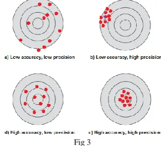
First though, a number of clarifications are essential in describing survey data, namely accuracy and precision [6].

Fig 3

ISSN: 2231-5381

http://www.ijettjournal.org

Page 52

convergence of the measurements. High precision have a narrow spread and small standard deviation.

In comparing the two parameters, there are instances of low accuracy and high precision as in b

(Fig. 3). Similarly in c is a representation of high accuracy and precision, and a, of low accuracy and precision, while in d is an instance of high accuracy and low precision.

Survey equipment are usually calibrated, and therefore assumed to be error free. Secondly, the surveying engineer is assumed to be skilled and competent in the use of instrument. Survey measurements are therefore in the category of high accuracy and high precision, often interchangeable.

A. Analogue Instrumentation

Fig 4

Survey analogue instruments include, levels and tapes, but are typified mainly by T2, Wild Universal Theodolite, as in Fig 4. Reading mechanism is characterized by a vernier scale micrometer for fine resolution. Thus, this least-count-possible is the basis of instrument standard and classification. Examples are then, the 1 sec,5 sec instruments etc.

Given stochastic nature of vernier readings, it is common to take several observations. An issue that arises, with standard of jobs, is the minimum number of rounds and round processing.

1. Rounds:

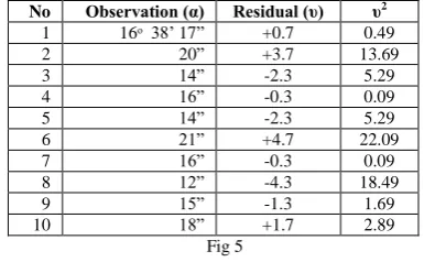
Consider ten equally reliable angle observations with values as given in Fig 5.

No Observation (α) Residual (υ) υ2

1 16ᵒ 38’ 17” +0.7 0.49

2 20” +3.7 13.69

3 14” -2.3 5.29

4 16” -0.3 0.09

5 14” -2.3 5.29

6 21” +4.7 22.09

7 16” -0.3 0.09

8 12” -4.3 18.49

9 15” -1.3 1.69

10 18” +1.7 2.89

Fig 5

The sample mean can be computed from (12). Thus:

𝛼 = 16ᵒ 38’ 16". 3

The standard error (deviation) by (14) is given as:

𝑠𝛼 = 𝜐2 𝑛 − 1=

70.10

10 − 1≈ ±2". 79

Similarly in respect of the mean, the standard error as computed from (15) gives:

𝑠𝛼 = 𝑠𝛼

𝑛= ±2.79 10= ±0". 88

Therefore the observed angle can be quoted as

𝛼 = 16ᵒ 38’ 16". 3 ± 0". 88

The relationship between the standard errors and number of rounds is obvious on inspection of the equation. If for instance, the mean is required at an error of ±1”, then

±1 = 2.79 /√n. Therefore n = 8 rounds

It should be explained that standard deviation in analogue measurement is a description of a particular observer. In specifying the number of rounds therefore, it is assumed that the spread and pattern of observations are unchanged. This criterion is normally used when specifying the number of rounds in any order of survey and instrument resolution.

2. Processing:

The challenge on processing is about determining and selecting good rounds for computation of the mean and rejecting bad observations. One of the established techniques, over the years, addresses outlying observations.

ISSN: 2231-5381

http://www.ijettjournal.org

Page 53

Chauvenet’s criterion [7, 8]. This technique defines an acceptable scatter, in a statistical sense, around the mean value from a given sample of N measurements. The criterion states that all data points should be retained that fall within a band around the mean that corresponds to a probability of 1-1/(2N).

In other words, data points can be considered for rejection only if the probability of obtaining their deviation from the mean is less than 1/(2N). This illustration is shown in Fig 6.

Fig. 6

The probability 1-1/(2N) for retention of data distributed about the mean can be related to a maximum deviation dmax away from the mean by using the Gaussian probabilities. For the given probability, the non dimensional maximum deviation τmax can be determined from the table where

τ𝑚𝑎𝑥 =𝛴(𝑥𝑖 − 𝑥 )𝑚𝑎𝑥 𝑆𝑥 =

𝑑𝑚𝑎𝑥 𝑆𝑥

and SX is the precision index of the sample. Therefore, all measurements that deviate from the mean by more than τmaxSX can be rejected. A new mean value and a new precision index can then be calculated from the remaining measurements. No further application of the criterion to the sample is allowed; Chauvenet’s criterion may be applied only once to a given sample of readings.

Consider a numerical example [5], consisting of rapid micrometer readings of a 1” theodolite, Fig 7.

No 𝒙𝒊 (secs) (𝒙𝒊 - 𝒙 ) (𝒙𝒊 - 𝒙 )2

1 41 -3.2 10.24

2 38 -6.2 38.44

3 38 -6.2 38.44

4 58 +13.8 190.44

5 47 +2.8 7.84

6 39 -5.2 27.04

7 46 +1.8 3.24

8 44 -0.2 0.04

9 41 -3.2 10.24

10 50 +5.8 33.64

Fig 7

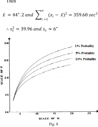
Then

𝑥 = 44". 2 𝑎𝑛𝑑 𝑛 (𝑥𝑖−

𝑖 =1 𝑥 )

2_{= 359.60 𝑠𝑒𝑐}2

∴ 𝑠𝑥2_{= 39.96 𝑎𝑛𝑑 𝑠𝑥≈ 6"}

Fig. 8

With respect to Fig 7 and reading the scale of probabilities in Fig 8, it can be seen that given a case of 1%, the maximum residual which can be accepted is 2.48 x 6” = 15”.Therefore the fourth reading is acceptable. Going higher however at 5%, the maximum acceptable residual is 2.28 x 6 = 13.7”. The fourth reading is rejected therefore and also at any higher level of probability.

The only drawback in this technique, as stated earlier, is that the criteria can only be applied once to a given sample. However as discussed in [9], Thompson variants can overcome this limitation with corresponding increase in number of observations.

Analogue instrumentation are nowadays mainly of historical significance and has given way to digital equipment, with revisions to techniques in round processing. Nevertheless, this tract highlights the origins of standard deviation as a metric in qualitative analysis.

B. Digital Instrumentation

Digital instruments are a major contrast to analogue options. Starting with electronic theodolites, electronic distance measurement and digital levels, evolutions has seen the emergence of computer measuring systems.

ISSN: 2231-5381

http://www.ijettjournal.org

Page 54

remote locations.

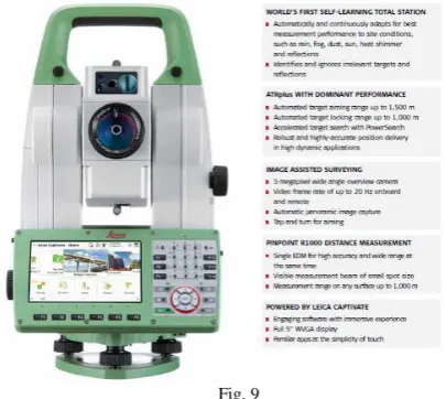
Fig. 9

Equipped in some instances with camera and scanner they are indeed resourceful platforms. The basic specifications are as follows:

Item Standard Deviation

Display Resolution

Remarks

Angle Measurement. Hz & V

1”, 2”, 3” and 5”

0.5”, 1” ISO

17123-3

Distance Measurement

1mm+5ppm 2mm+2ppm

Range of 1.5m-3500m

ISO 17123-4

These specifications highlight the major difference between analogue and digital system. In the former, standardization is based on resolution and standard deviation is associated with the surveyor. In this case, instruments have ISO certified values of standard deviation. These are population parameters that serve as references for computation of covariance of unknown positions.

The measure of precision of theodolites is expressed in terms of the experimental standard deviation (root mean square error) of a horizontal direction (HZ), observed once in both face positions of the telescope or of a vertical angle (V) observed once in both face positions of the telescope.

It should be noted that tests performed in laboratories would provide results which are almost unaffected by atmospheric influences. The costs for such tests are very high, and therefore they are not practicable for most users. Therefore, laboratory tests yield precisions much higher than those that can be obtained under field conditions [10].

1. Rounds:

Rounds are specified in view of required standard and order of survey, which in turn prescribes error margin for the mean of observations. Thus equation (13) may be recalled:

𝜎𝛼 = 𝜎𝛼 𝑛

However, the direction observations D, first have to be reduced to angles, and for which error propagation procedure is applicable. Thus from (7):

𝜎𝛼2_{= 𝜎𝐷}2_{+ 𝜎𝐷}2 _{. Let σD = 2” then 𝜎}

𝛼 = √8 = 2”.82

Suppose the error margin required for the mean observed angle is ±1”, the number of rounds is:

𝑛 = (𝜎𝛼 𝜎𝛼 )2

= (2.82 1 )2_{= 8 𝑟𝑜𝑢𝑛𝑑𝑠} If for instance the precision of instrument is 3”, the number of rounds becomes 18 and even more, as much as 50 at 5”. It becomes clear therefore that when the standard of survey is high, the use of equally high precision equipment is imperative.

2. Processing:

A number of important notes have to be taken into account, in comparison to analogue situation:

a. The instrument is the observer, rather than human. This is particularly true in robotic operations.

b. The standard deviation of observation is a population parameter, invariant and as stipulated by ISO 17123-3 and ISO 17123-4 certifications.

c. Given any set of rounds therefore, the task is to verify degree of congruence between 𝑠𝛼 of measurement and 𝜎𝛼, the instrument standard.

d. Noting that laboratory tests yield precisions much higher than those that can be obtained under field conditions, it should be expected that (𝑠𝛼 − 𝜎𝛼) > 0 .

Therefore given any rounds of observation, processing proceeds as follows:

1. Compute the standard deviation 𝑠_𝛼 of the set of observations n, n ≥Min.

a. Case (n < Min) Terminate Process

2. Taking note of (d), compare with instrument standard setting of 2𝜎𝛼.

a. Case (𝑠_𝛼− 2𝜎_𝛼) ≤ 0 , then all rounds is acceptable. Process ends. b. Case (𝑠_𝛼 − 2𝜎_𝛼) > 0 then

i. Determine the largest residual

ii. Delete from the list of rounds

ISSN: 2231-5381

http://www.ijettjournal.org

Page 55

where 𝑠𝛼 = 6". Let the precision of instrument be 𝜎𝐷= 2" then 𝜎𝛼 = 2”. 82. Then (𝑠𝛼 − 2𝜎𝛼) > 0, and case 2b is applicable. The largest residual is No 4 on the table. Delete item 4 and recompute to get 𝑠𝛼 = 4". 6. With the case of (𝑠𝛼− 2𝜎𝛼) ≤ 0 the process ends with selection of nine rounds. Note that this result is in agreement with the result of application of Chauvenet’s criterion, at a probability of 5%.

Further example involving precise measurements, comes from table in Fig 5. Let the standard deviation of instrument, 𝜎𝐷 be ±1”, for which 𝜎𝛼 = ±1”. 41. With 𝑠𝛼 = ±2". 79, and 2𝜎𝛼 = 2”.82, the result is (𝑠𝛼 − 2𝜎𝛼) < 0. Therefore all rounds are acceptable.

Fig 10

This algorithm has found application [11] in SMS, Fig 10 and is in concord with the rule-of-the-thumb approach that many surveyors apply when selecting rounds from observations.

Quantifying the margin by which laboratory tests is higher than field determination of standard deviation is not feasible, because of dynamic nature of atmospheric conditions. However, setting the margin in the range of 2.0𝜎𝛼, at a probability of 5% rejection has been satisfactory.

The variable Min may serve the purpose of restricting the number of deletions. By default Min, the minimum number of observations, is two.

III.RESULTS

Results analysis usually is the next task that follows the completion of a survey, and is a very important feature of any project management. In the days of analogue measurements, size of data tended to be in order of tens, yet it would take weeks or even months to arrive at conclusions.

The situation today is much different, with the dawn of data age. So rather than sample measurements, it is a case of data population, comprising of thousands of observations, involving equally very large number of positions. And it becomes a challenge how best to interpret the data, timely. Given that survey measurements follow Normal Distribution, it becomes pertinent to examine data through the prism and concept of standard deviation.

The study in this instance is as applies to Errors and Monitoring, with respect to zero centre line.

A. Error Analysis

Errors are in two categories, namely pre- computation checks for consistency in the network that is in form of loops and post computation that examines residual corrections to observations.

1. Loops Closure:

A loop often referred to as a cycle is a route that starts and returns to the same origin. In a perfect survey the same position is defined but in reality there will be some inconsistency that translates as closing errors. These errors also are representation of condition equations in the network and are therefore very important.

Fig 11

In Fig 11 is typical closing information in survey of a large level network involving 157 cycles. It is obvious that the histogram, in the limiting case, is a PDF representation of a normal distribution. Thus:

𝑓 𝑥 = 1 𝜎 2𝜋𝑒

−(𝑐𝑙𝑜𝑠𝑢𝑟𝑒 )2 2𝜎2

and

ISSN: 2231-5381

http://www.ijettjournal.org

Page 56

adopted in management as a parameter for analysis. Let Assessment be defined as 3𝜎_{𝑐𝑙𝑜𝑠𝑢𝑟𝑒}. If as indicated, this value is 14.9mm then approximately 99.7% of the area under the curve lies between ±14.9𝑚𝑚.The probability of closure higher than this value is 0.3%, and translates into a chance of 3:1000.

The advantages are as follows:

1. The Standard Closure at a glance provides information about the dispersion from Centre Line, a zero closure condition.

2. Assessment or any factor of 𝜎_{𝑐𝑙𝑜𝑠𝑢𝑟𝑒}can be a reference on which to compare with specified tolerance, and a basis to gauge performance and acceptability.

2. Residual Corrections:

Fig. 12

In Fig 12 is information regarding residuals to observations in the network. This example comprises of 310 edges in a level survey and for each of such run there is a correction. The final results are obtained by adding residual correction to each edge.

Grouping the information as in a histogram, it can be arrived as before that this is a PDF representation of a Normal Distribution. Hence:

𝑓 𝑥 = 1 𝜎 2𝜋𝑒

−(𝑐𝑜𝑟𝑟𝑒𝑐𝑡𝑖𝑜𝑛 )2_2𝜎2

and

𝜎𝑐𝑜𝑟𝑟𝑒𝑐𝑡𝑖𝑜𝑛 =

𝑐𝑜𝑟𝑟𝑒𝑐𝑡𝑖𝑜𝑛2 𝑛

Useful parameters are Standard Correction and Assessment as described earlier. The same advantages are applicable in providing spread about a zero-correction centre line and criterion for evaluation.

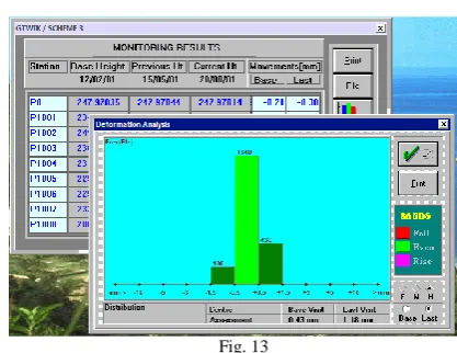
B. Monitoring Analysis

Fig. 13

Monitoring is one of the major applications of surveying in civil and environmental engineering. It requires very high precision surveys and in decades ago involved analogue measurements of critical points. These days besides Digital Levels and Total Stations, other instruments include 3D Scanners.

As a result the size of observations and points can be in thousands. The question to be answered rests on Movement Analysis. And that basically is to ascertain in very few parameters, any detection of significant movement, range and spread on base and last visits.

The information in Fig13 is a typical monitoring result, consisting of huge set of observed points. As such, the form of distribution is obvious.

Hence:

𝑓 𝑥 = 1 𝜎 2𝜋𝑒

−(𝑚𝑜𝑣𝑒𝑚𝑒𝑛𝑡 )2_2𝜎2

and

𝜎𝑚𝑜𝑣𝑒𝑚𝑒𝑛𝑡 = 𝑚𝑜𝑣𝑒𝑚𝑒𝑛𝑡2 𝑛

Standard Movement and Assessment are parameters for analysis. In the example, at 1.18mm against Last Visit, the probability of any movement in height above this assessment is 3:1000.

In context of any monitoring exercise, therefore, what constitutes a movement may be defined by specifying a value that can be compared with Standard Movement and derivatives.

ISSN: 2231-5381

http://www.ijettjournal.org

Page 57

IV.CONCLUSIONS

This paper charts ways in the evaluation and analysis of survey projects. It is coming timely at the advent of new technologies, in providing a means to cope with surge in data population. In the current trend, survey instruments now have standard deviation as specifications for errors and measures of precision. And taking it further, derivatives of the model can, in instances, serve as a metric in qualitative analysis.

The starting point of course, is field measurement and data collection. These are downloaded into field books, Fig 10, where they are processed in consistency with quoted instrument precision. Next is the collation of data into histograms. In the limiting function, and by Central Limit Theorem, they represent PDF of Normal Distribution. And from the conclusions emerge Assessment parameters, for Closure, Residual and Movement etc.

At a glance therefore, these important indices are available to assist prompt decision-making in quality management.

REFERENCES

[1] “Calculus Applied to Probability and Statistics”,

http://www.cengage.com/resource_uploads/downloads/143 9049254_242719.pdf.

[2] Department of Civil and Environmental Engineering, “Measurement Systems, Statistical and Error Analysis”, University of Buffalo, N.Y.

[3] MIT Sloane School of Management, “The Central Limit Theorem”, Massachusetts Institute of Technology, Cambridge. Summer 2003

[4] “Introduction to The Central Limit Theorem”, NCSSM Statistics Leadership Institute Notes, The Theory of Inference

[5] M. A. R. Cooper, “Fundamentals of Survey Measurement and Analysis”, Granada, © 1974, 1982 by M.A.R Cooper. [6] Department of Mathematics and Statistics, “Statistics:

Error”, Saint Louis University, St. Louis MO

[7] Department of Mathematics, “Chauvenet’s Criterion”, Ohio University, Athens, OH

[8] Sagar Sabade, Hank Walker, “Evaluation of Statistical Outlier Rejection Methods for IDDQ Testing”, Department of Computer Science, Texas A&M University, TX [9] E. S. Pearson, C. Chandra Sekar, “The Efficiency of

Statistical Tools and A Criterion for the Rejection of Outlying Observations”, Biometrika, Vol. 28, No. 3/4 (Dec., 1936), pp. 308-320

[10] ISO17123-3, “Optics and optical instruments -

Field procedures for testing geodetic and surveying instruments”, © ISO 2001