Vol. 08, Issue 01 (January. 2018), ||V1|| PP 85-93
A Multi-Period MPS Optimization Using Linear Programming
and Genetic Algorithm with Capacity Constraint
*M. S. Al-Ashhab
1,2*, Sufyan Azam
2, Shadi Munshi
2, Tarek M. Abdolkader
3,41Design& Production Engineering Dept. Faculty of Engineering, Ain Shams University – Egypt
2Dept. of Mechanical Engineering, College of Engineering and Islamic architecture, Umm Al-Qura University,
Makkah, Saudi Arabia.
3 Dept. of Basic Engineering Sciences, Faculty of Engineering, Benha University, Benha, Egypt.
4 Dept. of Electrical Engineering, College of Engineering and Islamic architecture, Umm Al-Qura University,
Makkah, Saudi Arabia. *Corresponding Author: M. S. Al-Ashhab
Abstract: This work presents a developed Master Production Scheduling (MPS) optimization model. The model is formulated in a mathematical programming form and solved using both linear programming (LP) and genetic algorithm (GA) tools. The model objective is to maximize the profit. The system consists of two potential suppliers that serve the factory to serve two customers. The model is solved using three Different Methods: (1) MATLAB linear Programming Algorithm, (2) MATLAB Genetic Algorithm, and (3) Using Evolver solver. The results of the
model are verified and the sensitivity analysis is done for some of the factors. Results obtained from the LP are
used to benchmark the results of the other two methods.
Keywords:Genetic Algorithm, MATLAB, Evolver, Linear Programming.
------ Date of Submission: 11-01-2018 Date of acceptance: 27-01-2018
---I. INTRODUCTION
Master Production Scheduling (MPS) is concerned mainly with optimization of the manufacturing activities in order to maintain desired profit. It acts as a communication tool with the business and delivers a manufacturing plan that targets the needs of the customer as well as the capabilities of the manufacturing organization assuring stable production. Many advances in MPS optimization have been attempted. N. P. Lin and L. Krajewski [1] developed a mathematical model for the MPS by an analytical approach using a rolling schedule. S. C. K. Chu [2] applied linear programming formulations for various levels of model complexity to optimize Material Requirements Planning (MRP) and master production scheduling (MPS). G. Ernani Vieira and P. C. Ribas [3] applied an artificial intelligence technique called Simulated Annealing to optimize a MPS problem. Other attempts included a genetic algorithm-based optimization technique for MPS, which was heavily dependent on the size of the manufacturing scenario [4]. Z. Wu et al. [5] also developed a working optimization method using the ant colony algorithm, which is a kind of population based heuristic bionic evolution of the system. Other researches solved production optimization problems using different solvers. Petr Klímek and Martin Kovářík [6] used MATLAB and Evolver software tools for determining the optimal production. Data preparation for Evolver was done in MS Excel Michalewicz [7] developed an evolution program for continuous time aggregate production an problems using Genetic Algorithm (GA) to determine a rate of production under varying types of demand and cost. Wang and Fang [8] formulated the same problem using a fuzzy linear programming model. Wang et al. [9] addressed the problem of joint marketing production decision aiming to maximize the net profit of a company. Wang and Fang [10] presented a fuzzy linear programming approach to solve aggregate production planning problems. Genetic algorithm is an approach for optimization, which is based on principles of biological evolution. It is usually used for the generation of high quality solutions for optimization problems. As in genetics, a chromosome is used which is formed of sequential arranged genes. Each one is controlling one or more characters. For chromosome handling, several operators have been proposed, most widely used are: selection, crossover, and mutation (Bäck and Schwefel) [11].
Another important software tool for optimization is “Evolver”. It is one of the fastest, most advanced commercial genetic algorithm based optimizer available. Evolver adopts powerful genetic algorithm based optimization techniques, which can find optimal solutions to unsolvable problems for standard linear and nonlinear optimizers [13]. In this paper, a developed mathematical MPS optimization model is proposed and solved using linear programming and genetic algorithm tools to maximize the profit. The system consists of two potential suppliers that feed the factory to serve two customers. The model is solved using various tools such as linear programming and genetic algorithm tools of MATLAB in addition to Evolver solver, which works as a supplement (Add-In) in MS Excel. The results of the model are then verified for accuracy and sensitivity analysis is performed for some of the factors. The rest of the paper is organized as follows: Section 2 presents both problem description and model formulation. In Section3, the model efficacy is verified and the solvers are evaluated. The effects of the factory capacity, shortage cost per unit, material cost per unit, non-utilized capacity cost, and the facility store capacity, on the optimal profit, are studied and discussed in section 4.
II. Problem description and model formulation
2.1 Problem description
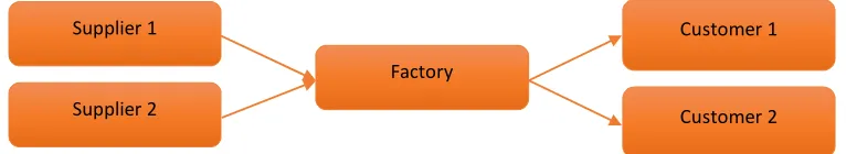
The problem consists of two approved suppliers that serve the factory to serve two customers as shown in Figure 1. The proposed research tackles the problem of production planning optimization in three periods for one product. The factory has a raw material and final good stores with limited capacities. The factory is enforced to receive an initial inventory and remains a pre-defined final inventory at the end of the planning periods.
Figure 1. Factory Relations Network.
2.2 Model formulation:
The model involves the sets, parameters and variables mentioned in [14].
2.2.1 Objective Function
The objective function for the model is to maximize the profit. The profit is calculated by subtracting the total cost from total revenue given in Equation 1.
Total Revenue = Q + I ∗ B ∗ P
∈ ∈
(1)
2.2.2 Total Cost Elements
Fixed cost = F (2)
Material cost = Q& ∗ B&∗ MatCost + II ∗ W)∗ MatCost − F+ ∗ W)∗ MatCost ∈
&∈,
(3)
Manufacturing cost
= Q ∗ B ∗ MH ∗ MC
∈ ∈
+ I ∗ B ∗ MH ∗ MC + I ∗ MH ∗ MC − F+ ∗ MH ∗ MC ∈
(4)
Supplier 1
Factory
Customer 1
Non − Utilized capacity cost = CAPH − Q ∗ B ∗ MH + I ∗ B ∗ MH ∗ NUCC
∈ ∈
(5)
Transportation cost
= Q& 6, ∗ B&∗ D& 6+ Q& 9, ∗ B&∗ D& 9 ∈
∈
+ Q ∗ B ∗ W)∗ T ∗ D 6+ I ∗ B ∗ W)∗ T ∗ D 6
∈ ∈ ∈
∈
(6)
Inventory holding costs = I+ ∗ B ∗ W)∗ HF + R ∗ B ∗ W)∗ HF
∈ 6; (7)
Shortage Cost = DEMAND6
∈..6 ∈
− Q + I B ∗ SCPU
?∈6…
+ DEMAND9 − Q + I ∗ B ∗ SCPU
?∈6.. ?∈6…
∈
(8)
2.2.3 Constraints
1) Balance Constraints
IA ≥ I ∈
(9)
R ;6 = I
∈
, ∀∈ (10)
Q& ∗ B&= &∈,
Q ∗ B ∗ W)+ I ∗ B ∗ W) , ∀∈ ∈
(11)
I ∗ B + IA = R ∗ B + I ∗ B
∈ (12)
I ∗ B + R ;6 ∗ B = R ∗ B + I ∗ B ,
∈
∀t ∈ 2
(13)
Q + I B ≤ DEAMND + DEAMND ;6 − Q ;6 + I ;6 B
F∈G
,
6→
∀t ∈ T, ∀c ∈ C (14)
R ∗ B = F+ (15)
Constraint (9-10) makes sure that the facility store avoids virtual storing.
Constraint (11) ensures that the quantity of inflow material to the factory from all suppliers equals the sum of the outflow from it.
Constraint (12-13) makes sure that the sum of beginning balance and additions to inventory equals the sum of ending balance and the withdrawal from inventory in all periods.
Constraint (14) makes sure that the sum of inflow to each customer does not exceed the sum of the current demand and the previously accumulated shortages for the product.
Constraint (15) makes sure that the residual inventory of the last period satisfying the required final inventory for the product.
2) Capacity Constraints
Q& ∗ B&≤ CAP& , ∀s ∈ S, ∀t ∈ T (16)
Q& ∗ B& ≤ CAPM , &∈,
∀t ∈ T (17)
R ∗ B ∗ w)≤ CAPFS&, ∀t ∈ T (19) Constraint (16) ensures that the outflow from each supplier to the factory does not exceed the supplier capacity at each period.
Constraint (17) makes sure that the sum of the material inflow to the factory from all suppliers does not exceed the factory material capacity at each period.
Constraint (18) ensures that the sum of manufacturing hours for outflows from the factory in each period does not exceed the manufacturing capacity.
Constraint (19) makes sure that the residual inventory at the factory store does not exceed its storing capacity at each period.
III. COMPUTATIONAL RESULTS
In this section, the model accuracy is verified and the solvers are evaluated.
3.1 Model Inputs
An example is assumed to verify the efficacy and efficiency of the model. The demands of all customers for products in the three periods are 850, 350, 750, 350, 750 and 850 unit respectively. The other parameters are considered as shown in Table1. The objective is to maximize the profit.
Table1. Verification model parameters.
Parameter Value
Number of products 1
Fixed costs($) 50000
Factory capacity (hrs.) 12000
Weight of product (Kg) 1
Price of the product 100
Material cost ($/kg) 10
Manufacturing cost ($/hr.) 10
Distance between suppliers and the factory 50.99 Manufacturing time for the product (hrs.) 1 Initial inventory of the product in the factory store 50 Final inventory of the product in the factory store 100 Capacity of each supplier in period (kg), 1200 Capacity of the factory store (Kg) 2000
Supplier batch size 10
3.2 Model Outputs and Discussion
The model is solved using MATLAB and Evolver softwares and ran on an Intel ® Core™ i3-2310 MCPU@ 2.10 GHz (3 GB of RAM). Regarding to the GA parameters; population size N = 200, number of generations G = 1000, probability of crossover Pc = 7.0 and probability of mutation Pm = 0.01
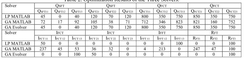
Table 2 shows the results obtained by solving the model using Linear Programming (LP) optimization tool in MATLAB, GA optimization tool in MATLAB, and GA optimization solver in Evolver. The optimal maximum values achieved using LP MATLAB and GA Evolver solvers are equals as 145,882$. However, the optimal maximum value achieved using GA MATLAB solver is 140,865 $.
Table 2. Optimization Results of the Three Solvers.
Solver QSFT QSFT QFCT QFCT
QSFT11 QSFT12 QSFT13 QSFT21 QSFT22 QSFT23 QFCT11 QFCT12 QFCT13 QFCT21 QFCT22 QFCT23 LP MATLAB 45 0 40 120 70 120 800 350 750 850 350 750 GA MATLAB 72 17 92 105 38 71 712 346 823 821 160 752 GA Evolver 45 0 40 120 70 120 800 350 750 850 350 750
Solver IFCT IFCT IFFT RFT
IFCT 11 IFCT 12 IFCT 13 IFCT 21 IFCT 22 IFCT 23 IFFT 11 IFFT 12 IFFT 13 RFT1 RFT2 RFT3
LP MATLAB 50 0 0 0 0 0 0 0 100 0 0 100
GA MATLAB 237 45 53 36 32 0 4 213 0 247 47 100
GA Evolver 0 0 100 50 0 0 0 0 0 0 0 100
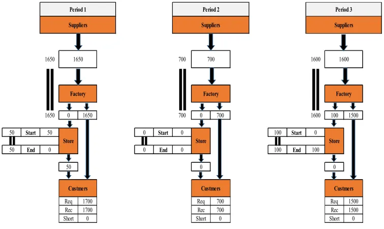
Figure . The suppliers supplied 1650 units to the factory during the first period but the customer demand in this period was1700, so to balance the demand 50 units were taken from the factory store initial inventory. The customer demand for the second period meets the factory production capacity, so no units were stored in the factory store. By the end of the last period, the factory, in addition to satisfying customer demands, was constrained to store 100 units. The Flow balance in Figure 2 for the above problem verifies the results obtained by the three solvers shown in Table 2.
Figure 2. Flow balancing using the three solvers.
For discovering the reason of getting near optimal solution from MATLAB GA optimization tool,
another small-scale problem of smaller number and values of variables is assumed and solved. In the small-size
problem, shown in Figure 3, the number of variables is reduced to be15variables instead of 24 variables in the
main problem by reducing both the number of suppliers and the number of customers into one instead of two. The
optimal maximum value achieved using Evolver is equal to the value obtained using the LP solver of 145,882 $
Figure 3. Small-size factory relations network.
The small-size problem has been solved using both genetic algorithm optimization tools in addition to the LP tool; Evolver and MATLAB. All solvers gave the same results as shown in Table3. The optimal maximum value achieved using these three solvers is -79,194$.
Table3. Small-size problem results using all mentioned Optimization tool.
SOLVER QSFT QFCT IFFT
QSFT11 QSFT11 QSFT11 QFCT11 QFCT12 QFCT13 IFFT 11 IFFT 12 IFFT 13
LP MATLAB 80 35 85 800 350 750 0 0 100
GA MATLAB 80 35 85 800 350 750 0 0 100
GA Evolver 80 35 85 800 350 750 0 0 100
Solver IFCT RFT
IFCT 11 IFCT 12 IFCT 13 RFT1 RFT2 RFT3
1650 0 1650 700 0 700 1600 100 1500
50 Start 50 0 Start 0 100 Start 0
50 End 0 0 End 0 100 End 100
50 0 0
Req 1700 Req 700 Req 1500
Rec 1700 Rec 700 Rec 1500
Short 0 Short 0 Short 0
Period 1 Period 2 Period 3
Suppliers
1650 700 1600
Suppliers Suppliers
1650 700 1600
Custmers Custmers Custmers
Factory Factory Factory
GA MATLAB 50 0 0 0 0 100
GA Evolver 50 0 0 0 0 100
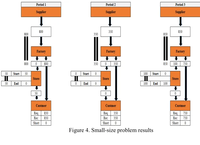
The weight flow balance during the three periods of time of the small sized problem is shown in Figure 4. 800 units were supplied to the factory by the supplier during the first period and the customer demand in this period was 850 so to balance the demand, 50 units were taken from the factory store initial inventory. The customer demand, for the second period, meets the factory production capacity of 350 units hence no units were stored in the factory store. By the end of the last period, the factory was constrained to store the 100 units in addition to satisfying customer demand of 750 units.
Figure 4. Small-size problem results
IV. Sensitivity Analysis
In this section, the effects of the factory capacity, shortage cost per unit, material cost per unit, non-utilized capacity cost, and the facility store capacity, on the optimal profit, are studied and discussed.
4.1 Factory Capacity Effect
Figure 5. Factory capacity effect.
capacity cost, such as overhead and depreciation cost of the machines. No results are available below 100 units of the factory capacity since the required final inventory should be exact100 units.
4.2 Shortage Cost Per Unit Effect
Figure 6. Shortage cost per unit effect.
Figure 6 presents the effect of changing the shortage cost per unit on the optimal profit. Since the demand was satisfied in all periods, there is no shortage and the shortage cost per unit has no effect on the profit.
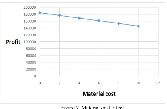
4.3 Material Cost Effect
Figure 7. Material cost effect.
4.4 Non-Utilized Capacity Cost Effect
Figure 8. Non-utilized capacity cost effect.
Figure 8 presents the effect of the non-utilized capacity cost on the optimal profit. It can be noticed that the increase of the non-utilized capacity cost decreases the profit whereas this increase increases the total cost.
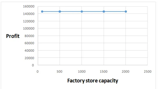
4.5 Factory Store Capacity Effect
Figure 9. Factory store capacity effect.
Figure 9 presents the effect of the factory store capacity on the optimal profit. Since there is no storage between the periods, the factory store capacity has no effect on the profit. The demand is satisfied directly during all the periods and the final inventory cost is assigned to the fourth period, which is not included in this planning horizon. No results are available below 100 units of the factory store capacity to satisfy the constraint of the required final inventory of exact 100 units.
V. CONCLUSION
effects of the factory capacity, shortage cost per unit, material cost per unit, non-utilized capacity cost, and the facility store capacity, on the optimal profit, are studied and discussed.
REFERENCES
[1]. N.-P. Lin and L. Krajewski, "A Model for Master Production Scheduling in Uncertain Environments," Decision Sciences, vol. 23, pp. 839-861, 1992.
[2]. S. C. K. Chu, "A mathematical programming approach towards optimized master production scheduling," International Journal of Production Economics, vol. 38, pp. 269-279, 1995/03/01/ 1995.
[3]. G. Ernani Vieira * and P. C. Ribas, "A new multi-objective optimization method for master production scheduling problems using simulated annealing," International Journal of Production Research, vol. 42, pp. 4609-4622, 2004/11/01 2004.
[4]. M. M. Soares and G. E. Vieira, "A new multi-objective optimization method for master production scheduling problems based on genetic algorithm," The International Journal of Advanced Manufacturing Technology, vol. 41, pp. 549-567, 2009/03/01 2009. [5]. Z. Wu, C. Zhang, and X. Zhu, "An ant colony algorithm for master production scheduling optimization," in Proceedings of the 2012
IEEE 16th International Conference on Computer Supported Cooperative Work in Design (CSCWD), 2012, pp. 775-779. [6]. P. Klímek and M. Kovárík, "Genetic Algorithms as a Tool of Production Process Control," Journal of Systems Integration, vol. 5, p.
57, 2014.
[7]. Z. Michalewicz, Genetic algorithms+ data structures= evolution programs: Springer Science & Business Media, 2013. [8]. D. Wang and S.-C. Fang, "A genetics-based approach for aggregated production planning in a fuzzy environment," IEEE
Transactions on Systems, Man, and Cybernetics-Part A: Systems and Humans, vol. 27, pp. 636-645, 1997.
[9]. P. P. Wang, G. R. Wilson, and N. G. Odrey, "An on-line controller for production systems with seasonal demands," Computers & industrial engineering, vol. 26, pp. 565-574, 1994.
[10]. R.-C. Wang and H.-H. Fang, "Aggregate production planning with multiple objectives in a fuzzy environment," European Journal of Operational Research, vol. 133, pp. 521-536, 2001.
[11]. T. Bäck and H.-P. Schwefel, "An overview of evolutionary algorithms for parameter optimization," Evolutionary computation, vol. 1, pp. 1-23, 1993.
[12]. M. Saraswat, "Genetic Algorithm for optimization using MATLAB," International Journal of Advanced Research in Computer Science, vol. 4, 2013.
[13]. Palisade. (2010). Guide to Using Evolver. Available: www.crystalballservices.com
[14]. M. S. Al-Ashhab, T. Attia, and S. M. Munshi, "Multi-Objective Production Planning Using Lexicographic Procedure," American Journal of Operations Research, vol. 7, p. 174, 2017.