Volume 8, Issue 6 (September 2013), PP.01-11
Modeling, Simulation and Control of Temperature and
Level in a Multivariable Water Tank Process*
Vassilios Tzouanas
1, Sanjo Peter
2, Matthew Stevenson
3, Truong Doan
4 1,2,3,4University of Houston-Downtown, One Main Street, Houston, TX 77062, USAAbstract:- The project is concerned with the design of a water tank process and experimental evaluation of feedback control structures to achieve water level and temperature control at desired set point values. The manipulated variables are the pump power, on the water outflow line, and heat supply to the tank. Detailed, first principles-based, dynamic models as well as empirical models for this interactive and multivariable process have been developed and used for controller design. Furthermore, this experimental study entails and discusses the design of the water tank process and associated instrumentation, real time data acquisition and control using the DeltaV distributed control system (DCS), process modeling, controller design, and evaluation of the performance of tuning methodologies in a closed loop manner.
Keywords:- Process control, Modeling, Simulation, PID Control, Tuning
I.
INTRODUCTION
The Control and Instrumentation program at the University of Houston - Downtown includes a number of courses on process control, process modeling and simulation, electrical/electronic systems, computer technologies, and communication systems. To meet graduation requirements for the degree of Bachelor of Science in Engineering Technology, students must work in teams and complete a capstone project. This project, also called Senior Project in our terminology, provides students with an opportunity to work on complex control problems, similar to ones encountered in the industry, and employ a number of technologies and methods to provide a practical solution.
In general, the Senior Project entails the design and construction of a process, identification of key control objectives, specification and implementation of required instrumentation for process variable(s) monitoring and control, real time data acquisition and storage methods, modeling of the process using empirical and/or analytical methods, design and tuning of controllers, and closed loop control performance evaluation. Equally important to these technical requirements are a number of non-technical requirements focusing on project management, technical writing, presentation of technical topics, teamwork and communication. This paper presents the results from a senior project which aims to simultaneously control the level and temperature of water in a tank. Such objectives are important to the process industries concerned with materials and energy control.
The remaining of the paper is organized as follows. Section II discusses the process under consideration and the control objectives. Sections III refers to the instrumentation required to measure and control key process variables. Section IV presents the computing platform which is a distributed control system (DCS). Section V presents the dynamic modeling results based on first principles. Section VI presents empirical modeling, tuning and closed loop results for the water level and temperature. Section VII summarizes main results and is followed by references.
II.
THE
PROCESS
AND
CONTROL
OBJECTIVES
A schematic and picture of the process is shown in Figure 1. The water tank has a constant cross sectional area. The water height is being affected by the flow in and the flow out. The flow in to the tank is not available for control purposes but can be manually adjusted to simulate a process disturbance. The water outflow depends on the power supplied to the pump which is available for manipulation and control of the water level in the tank. A heating element provides the required energy to maintain a desired water temperature by adjusting the electrical power to it.
The control objective is to maintain the water level (measured by transmitter LT) and temperature (measured by transmitter TT) at desired setpoint values using closed loop feedback control strategies which employ PI controllers (LC and TC, respectively) on a Delta V distributed control system. Figure 2 shows the control strategy to achieve this objective.
Fig. 1: Schematic and Picture of the Water Tank
Fig. 2: Control Strategy for the Water Tank
As shown in Fig. 2, one PI controller is used to maintain material inventory (i.e. water level) in the tank by adjusting the power to the pump. Also, another PI is used to control the water temperature at a desired setpoint value by adjusting the power to the heating element.
III.
PROCESS
INSTRUMENTATION
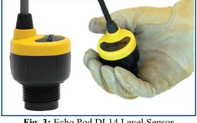
To achieve water level and temperature control, a number of instruments are used. Water level is measured using a general purpose EchoPod DL14 sensor with 4-20mA signal output, see [1]. For the purpose of this project the level transmitter is calibrated to read up to 25 inches maximum. The level transmitter is connected to the DCS input card. Fig. 3 shows a picture of the level sensor.
Fig. 3: Echo Pod DL14 Level Sensor
Fig. 4: Attwood Tsunami Aerator Pump
A pulse width modulation (PWM) circuit is used to adjust the speed of the DC motor to manipulate the flow out from the tank, which in turn controls the level of the tank. A LM324 IC based PWM circuit is used to control the speed of the motor. The PWM circuit converts in coming 1 to 5 volt signal to an average 0 to 12 volt output to control the speed of the motor. The 4 to 20 mA output from the DeltaV is converted to a 1 to 5 volt signal using a resistor in parallel with the output. This 1 to 5 volt signal serves as the reference voltage for the PWM circuit. The circuit compares the reference voltage to an internally generated saw tooth voltage to control the average output to the motor. The average voltage output to the motor depends on the width of the 12 volt pulses that are sent to the motor.
Water temperature is measured using a Type K thermocouple with a sensitivity of approximately 41 µV/°C (Fig. 5)
Fig. 5: HTTC36-K-18G-6 K Type Thermocouple
The power to the heating element is controlled using a zero crossing Watlow controller, see [3], (Fig. 6). The Watlow controller takes 4 to 20 mA as input and determines the number of cycles reaching the heating element from a 60 Hz alternating current depending on the input to achieve continuous control of the heater. The power for the heating element comes from a 20 Amps, 220 Volt, 2 Phase disconnect switch. The maximum power that can be drawn by the heater is limited by the disconnect switch.
Fig. 6: Watlow DIN-A-MITE Power Controller
IV.
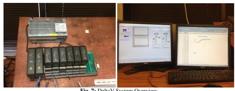
THECONTROLPLATFORMFig. 7: DeltaV System Overview
The strategy for level and temperature control has been implemented using two PI controllers. Part of the system configuration and implementation is the development of a user interface which allows the user to oversee the control of the tank process. Figure 8 shows this user interface along with the faceplates of the level and temperature controllers. Using these faceplates, the user can change the mode of the controllers (Auto/Manual), adjust the setpoint of the controllers (in auto mode) or the controller output (when in manual mode), and even fine tune the controllers by specifying the values for the proportional gain and integral time (or reset in DeltaV terminology). Details on system configuration and interface development are beyond the scope of this work and thus omitted.
Fig. 8: Operator Interface with Controller Faceplates and Trending Capabilities
V.
ANALYTICAL
MODEL
In order to design and tune the level and temperature controllers, models describing the impact of pump power on level and heating element power on temperature are required. Such models can be developed using empirical methods (i.e. step testing the process) or analytically using material and energy balances. The development of the analytical models is described in the following for the water level and temperature.
1) Level Model: Referring to Fig. 1, the two inputs to this model are the water flow in, Fi, and flow out, Fo, from the tank. Assuming constant water density, , and tank cross sectional area, A, a material balance around the tank yields:
Then,
If,
then
(1)
Equation (1) is the time domain model between the water level, h, and the flow in and pump power (in % of scale). To develop the transfer function, equation (1) is Laplace transformed which yields:
(2)
From equation (2), the transfer function between tank level, h, and pump power is:
s
A
K
s
V
s
h
v v
)
(
)
(
(3)Since data is gathered every 5 seconds, a time delay of 5 sec (or 0.083 min) is added to the level transfer function. Thus, to tune the PI controller, the transfer function in equation (4) is used:
s
A
e
K
s
V
s
h
v sv
0.083)
(
)
(
(4)
For the water tank, the following operating data applies: Cross sectional area, A: 225 in2
Maximum level, h: 25 in
Max pump flow, Fo,max: 100 gph = 1.67 gpm
Pump constant, Kv: 0.0167 gpm/% speed = 3.85 in3/min/%speed
Using this data, equation (4) yields:
s
e
s
A
e
K
s
V
s
h
s
G
s s v v A PL 083 . 0 083 . 0 ,0684
.
0
)
(
)
(
)
(
(5)Thus, Equation (5) gives the transfer function between the water level (in %) and the pump power (in %). It can be used to tune the level PI controller according to any chosen tuning methodology.
2) Temperature Model: The model describing the effect of power to the heating element on the water temperature is derived by combining material and energy balances. Also, the following assumptions are being made:
a. Water density and heat capacity remain constant b. There is perfect water mixing in the tank
c. The water level is kept constant (i.e. flow in = flow out) d. The tank cross sectional area is constant
e. The inlet water temperature is constant f. Heat losses to the surroundings are minimal
Then, using the previous assumptions, an energy balance around the tank gives:
h h P i i P p
P
K
T
F
c
T
F
c
dt
T
c
m
d
0)
(
where:cP: water heat capacity water density Fi: water flow in
Ti: inlet water temperature Fo: water flow in
T: water temperature
Kh: gain of power to heating element Ph: power to heating element (in % of scale)
Since:
h
A
m
Then: h P h i i h P h i i h h P i i P p P F c K T T F F dt dT F h A or P c K T F T F dt dT h A or P K T F c T F c dt dT h A c 0 0 0 0 0
Since, it is assumed that the level is held constant, Fi = Fo. Then,
h P h i
P
F
c
K
T
T
dt
dT
F
h
A
0 0
Assuming deviation variables, Ti to remain constant, and Laplace transforming the above equation, it yields:
1
)
(
)
(
)
(
)
(
)
(
)
(
]
1
)
[(
)
(
)
(
)
(
)
(
0 0 , 0 0 0 0
s
F
h
A
F
c
K
s
P
s
T
s
G
or
s
P
F
c
K
s
T
s
F
h
A
or
s
P
F
c
K
s
T
s
T
s
F
h
A
P h h A PT h P h h P h
The above equation gives the analytically derived transfer function between the power to the heating element (in % of scale) and water temperature. Using the steady state conditions for the water tank as shown in Table 1, the following analytical process model is obtained:
Table 1: Water Tank Data Water Tank Steady State Conditions
Variable Value Units
Water flow out 92.25 in3/min
Water heat capacity 4.18 J/(g K)
Water density 1 g/cm3
Water height (%) 50 %
Tank cross sectional area 225 in2
Maximum power to heating element
1040 W
Heating element power gain 624 J/(min %)
Thus, the process gain is 0.095 C/% while the time constant is 29.22 min.
VI.
EMPIRICAL
MODELING,
TUNING
AND
CLOSED
LOOP
CONTROL
Empirical models between controlled and manipulated variables are being developed by collecting and analyzing process data gathered under controlled, open loop conditions by stepping the manipulated variables. Using such models and certain tuning methods, initial tuning parameters for the water level and temperature PI controllers are calculated. Finally, the closed loop performance of the PI controllers is tested for setpoint changes and the interaction of the two control loops is being accessed.
1) Empirical Modeling for Level Controller: The water tank level is held constant by equalizing the water flow out and the flow in. Then, the flow out is changed in a step wise manner and the level response is being observed. A series of step changes is introduced while the water level is maintained within range. As expected, the level behaves like an integrating (or ramp) process. Using step test data, an average time delay (in min) and gain ( in % of level/min per % of power) were calculated. These values are as follows:
Level Process Gain:
power
level
K
PL%
min
/
%
073
.
0
Level Time Delay:
min
14
.
0
sec
5
.
8
L
Thus the empirical transfer function between the tank level and the pump speed is:
s
e
s
e
K
s
G
s s
PL E
PL
L
0.14,
073
.
0
)
(
(7)
By comparing the analytical transfer function, equation (5), and the empirical transfer function, equation (7), there is good agreement between both methods for this particular process. To tune the PI level controller the model given by equation (7) is used.
2) Tuning the Level Controller and Closed Loop Results: Using the IMC tuning method5, and for various values of the closed loop time constant, c, the tuning parameters are shown in Table 2 with the integral time in seconds as required by DeltaV.
Table 2: Level Controller Tuning using the IMC Method
c (sec)
Kc
(%speed/%level/min)
i (sec)
8.5 73.32 25.2
17 54.35 42.0
25.5 42.80 58.8
34 34.5 76.5
42.5 29.89 92.4
51 25.95 109.2
Based on the data shown in Table 2, it is concluded that as the desired closed loop time constant increases, the tuning of the controller is less aggressive (lower gain and longer integral time).
Fig. 9: Level Control for Different Values of the Filter Time Constant
By comparing the different system responses, it seems that when Kc=34.5 and ti=76.5 sec, the level responds very well to setpoint changes. However, the manipulated variable response is still very noisy. By filtering the level measurement using a filter with time constant of 10 seconds, the closed system response is improved (Fig. 10). The reduction in the movement of the manipulated variable (pump power) is noticeable.
Fig. 10: Level Setpoint Response with Kc=34.5 and ti=76.5 sec and Filter Time Constant of 10 sec.
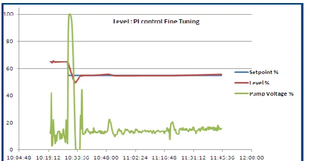
In spite of the performance improvement achieved, as shown in Fig. 10, by filtering the controlled variable (level), it appears that the controller is still tightly tuned. Further manual adjustments to the tuning parameters yield the response shown in Fig. 11. The conclusion is that using modeling techniques and appropriate tuning methods, good initial tuning parameters can be obtained. However, final manual adjustments may be required to further improve closed loop control performance.
3) Empirical Modeling and Control of Water Temperature: A number of step changes are made to the power to the heating element and the water response is observed. The response was modeled as that of a self-regulating process as shown in Fig. 12.
Fig.12: Temperature response to heating element power changes and modeling results
Fig. 12 shows the process variable (blue line of top plot) as it varies in response to changes to the heating element power which is indicated as controller output in the bottom plot (blue line). The red line in the top plot is the model prediction of the process variable. These results have been obtained using PAS’s TuneWizard software6. Also, shown in Figure 12 are the modeling results for a first order plus dead time model. Using the PAS TuneWizard, the calculated parameter values for a first order plus dead-time model, as shown in equation (8), are:
(
)
1
)
(
)
(
,
s
e
K
s
P
s
T
s
G
P s p
h E
PT
(8)
Process gain: KP = 0.101 C/% power Time constant: p = 26.8 min
Time delay: = 3.71 min
Comparing the analytical and empirical temperature models from equations (6) and (8), respectively, it is concluded that there is good agreement. The analytical model does not show a time delay because of the perfect mixing assumption. For tuning purposes, the empirical model will then be used.
Using the IMC tuning method5, and for various values of the closed loop time constant, c, the tuning parameters are shown in Table 3 with the integral time in seconds as required by DeltaV.
Table 3: Level Controller Tuning using the IMC Method
c (min) Kc (%/C) i (min) i (sec)
3.71 8.70 26.80 1608
11.13 7.00 26.80 1608
18.55 5.85 26.80 1608
22.26 5.41 26.80 1608
26.80 4.95 26.80 1608
29.68 4.70 26.80 1608
37.10 4.15 26.80 1608
Using the tuning the tuning methods included in the PAS TuneWizard, the calculated tuning parameters are: Kc = 53.9 and i = 1071 sec with a detuning factor of 0.67. The detuning factor was set to 0.67 to improve closed loop performance while the system robustness was still acceptable.
Based on the open loop transfer of the temperature, it is expected that the temperature loop will respond slowly. To test the impact of different tuning parameters, the PAS TuneWizard simulation option was used. In Fig. 13, the simulated closed loop results for two different sets of tuning parameters are shown. The dark blue line corresponds to the tuning of Kc = 53.9 and i = 1071 sec while the pink line corresponds to Kc = 63 and i = 720 sec.
In the same Fig. 13, the closed loop system response to setpoint changes and the disturbance rejection performance are shown. At, least in simulation, the Kc = 63 and i = 720 sec tuning yields slightly improved results and was tried on the experimental process.
Fig. 13: Setpoint and Disturbance Rejection Performance (Simulated)
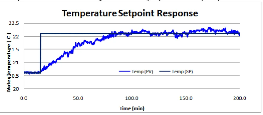
Experimental results are shown in Fig. 14. Indeed the step response shows acceptable performance.
Fig.14: Experimental Results for Temperature Setpoint Response (Kc = 63, i = 720 sec)
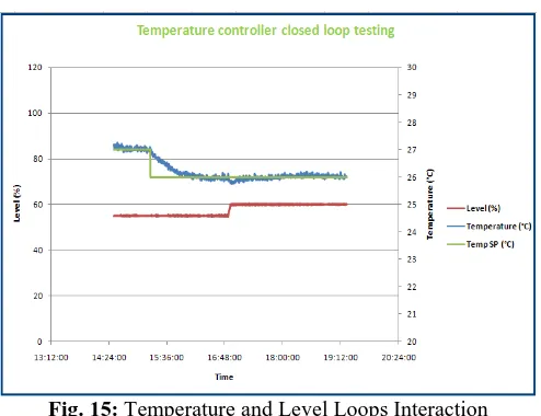
Fig. 15: Temperature and Level Loops Interaction
VII.
CONCLUSIONS
The paper was concerned with the design of two feedback, single input/single output control structures to control an interactive, multivariable, experimental process. The controlled variables are the tank water level and temperature. Modeling results using analytical, first principles based methods, and empirical, step test based, approaches were presented. There was close agreement between the analytical and empirical models. Tuning of the PI controllers was done using the IMC method and the methods available within PAS TuneWizard. For improved closed loop performance, fine tuning of the PI controllers was required.
REFERENCES
[1]. Flowline website, www.flowline.com[2]. Attwood Marine Website, www.attwoodmarine.com [3]. Watlow Worldwide website, www.watlow.com [4]. Emerson Website, www.emerson.com
[5]. Rivera D.E., Morari M, Skogestad S., “Internal model control. 4. PID controller design”, Ind. Eng. Chem. Process Des. Dev. 1986; 25:252–65.