Adaptive DKT Finite Element for Plate Bending
Analysis of Built-up Structures
Pichayen Bhothikhun
1and Pramote Dechaumphai
1*1
Department of Mechanical Engineering, Chulalongkorn University, Phyathai Road, Patumwan, Bangkok 10330, Thailand.
* E-mail: [email protected], Tel: (662) 2186621, Fax: (662) 2186621
Abstract-- Discrete Kirchhoff Triangle (DKT) which provides high solution accuracy for the plate bending analysis combined with the adaptive meshing technique is presented. The finite element formulation of the DKT plate bending element together with the CST membrane element used for modeling such 3D plate structures is derived and the associated finite element matrices are presented. An adaptive meshing technique is applied to generate small elements in the regions of high stress gradient to improve the solution accuracy. Larger elements are placed in the other regions to reduce the problem unknowns and thus the computational time. The effectiveness of the combined method is evaluated by several problems. Results show that the combined method can improve the solution accuracy and reduce the computational effort.
Index Term-- plate bending, DKT, finite element method, adaptive mesh, built-up structures
1.INTRODUCTION
The finite element method has been widely used in plate structural analyses. Numerous plate bending elements have been developed during the past decades to improve the efficiency and solution accuracy in the finite element prediction of plate structural responses [1-5]. In the present paper, triangular element is considered because it can provide high flexibility in construction of finite element models with different element sizes for complex geometries. One of the triangular element types which provide high solution accuracy for the plate bending analysis is the Discrete Kirchhoff Triangle (DKT) [6-9]. This triangular element consists of three corner nodes with 9 degrees of freedom (dof). Such 3D plate structures are commonly modeled by using two-dimensional membrane and plate bending elements. Herein, the DKT plate bending element is combined with the constant strain triangular (CST) membrane element because of its simplicity in implementation and the equivalence of the number of node in each element. The CST element, which assumes a linear displacement distribution over the element, provides less accurate solution than other higher order triangular membrane elements. However, the solution from the CST element can still converge to the actual solution as the mesh is more refined. On the contrary, the higher order elements require more degrees of freedom than the CST does, and they always face with the membrane locking problem [10,11]. This leads to the necessity of improving the solution accuracy of the superposition of the DKT and CST element.
The adaptive meshing technique has been used to obtain much higher solution accuracy in both of the fluid and structural problems [12,13]. This technique generates small clustered elements in the regions of high stress gradients to obtain higher solution accuracy. At the same time, larger elements are generated in the other regions to reduce the total number of unknowns and a computational time. Because the technique generates appropriate element sizes automatically, it is suitable for complex plate structural problem where a priori knowledge of the solutions does not exist. Herein, the adaptive meshing technique has been combined with the DKT and CST elements for structural analysis of built-up structures under mechanical responses. The performance of the combined method is evaluated by several problems in which the adaptive mesh solutions will be compared with the fine mesh solutions.
The governing differential equations for predicting structural response will be presented first. The corresponding finite element equations and the associated element matrices will then be derived and presented. Basic concepts of the adaptive meshing technique and the selection of the meshing parameters used for construction the new meshes will be explained. Finally, the effectiveness of the DKT element and the adaptive meshing technique are evaluated by several examples.
2.GOVERNING EQUATIONS
The governing equations for the in-plane deformation and the transverse deflection of a plate that lies in a local x-y
coordinate system are briefly described herein.
2.1 In-Plane Deformation
The equations for the in-plane deformation are governed by the two-dimensional equilibrium equations after neglecting the in-plane body forces [14] as
0
xy x
x y
(1)
0
xy y
x y
For the plane stress case, the stress components
x, y andxy
are related to the strain components by Hooke’s law [14] as
C
(3)where
and
vectors are defined by,
Tx y xy
(4)
T u v u vx y y x
(5)
The material stiffness matrix
C is given by
21 0
1 0
1
1
0 0
2
E C
(6)
2.2 Transverse Deflection
The equation for the transverse deflection w in the z -direction normal to the x-y plane of a thin plate with a constant thickness of t whose middle plane is coincident with the x-y
plane is given by the equilibrium equation [15] in the form of
4 4 4
4 2 2 2 4 ,
w w w
D p x y
x x y y
(7)
where p(x,y) is the applied lateral load normal to the plate and
D is the bending rigidity. The bending rigidity is defined by
3
2
12 1
Et D
(8)
where E is the modulus of elasticity, t is the thickness of the plate and is Poisson’s ratio.
3.FINITE ELEMENT EQUATIONS
The Constant Strain Triangle (CST) and the Discrete Kirchhoff Triangle (DKT) finite elements are used for the in-plane deformation and the transverse deflection, respectively.
3.1 Constant Strain Triangle (CST)
The three-node CST element assumes a linear displacement distribution over the entire element. The element equations can be derived by applying the method of
weighted residuals [16] to the governing differential equations, Eq. (1) and (2), which leads to the element equations in the form of
Km
m Fm (9)where the vector
m contains the element nodal unknowns of the in-plane displacements in the element local x-ycoordinate directions. With two in-plane displacements (u and
v) per node, there are six unknowns per element. The element stiffness matrix,
Km , that appears in Eq. (9) is defined by
Tm m m m
K B C B tA (10)
where
Bm is the strain-displacement interpolation matrix (the closed form of
Bm can be derived in terms of differences of nodal coordinates and given in Ref. [14]). The vector
Fm on the right-hand-side of Eq. (9) contains the applied mechanical forces at element nodes.3.2 Discrete Kirchhoff Triangle (DKT)
The derivation of the Discrete Kirchhoff Triangle (DKT) element equations is based on the following assumptions [8]: (1) both the x- and y-twist angles vary quadratically over the element; (2) the transverse shears are zero at the tip nodes; (3) the transverse deflection is in the form of a cubic function over the element; and (4) the twist angles normal to the element sides vary linearly. The finite element equations are derived by applying the method of weighted residuals to the plate bending equilibrium equation (Eq. (7)) leading to the finite element equations in the form of
Kb
b Fb (11)where the vector
b contains the element nodal unknowns of the transverse deflection and rotations. Each node has a transverse deflection in the z-direction and the two rotations about the x- and y-directions. Thus, there are nine degrees of freedom per element. The element stiffness matrix
Kb and the nodal force vector due to the applied loads
Fb are defined by
Tb b b
A
K
B D B dA (12)
Tb p
A
F
N p dA (13)31 12
31 12
31 12 31 12
1 2 x x y y b y y x x H H y y H H
B x x
A
H H
H H
x x y y
(14)
where Hx , Hy , Hx
and
y H
are
6 5 6
6 5 6
6 5 6
6 4 6
6 4 6
6 4 6
4 5
4 5
4 5
1 2 1 2
4 6 1 2
1 2 1 2
2 6 1 2
x
P P P
q q q
r r r
P P P
H
q q q
r r r
P P q q r r (15)
6 5 6
6 5 6
6 5 6
6 4 6
6 4 6
6 4 6
4 5
4 5
4 5
1 2
1 1 2
1 2 1 2
1 1 2
1 2
y
t t t
r r r
q q q
t t t
H
r r r
q q q
t t r r q q (16)
5 5 6
5 5 6
5 5 6
4 6
4 6
4 6
5 4 5
5 4 5
5 4 5
1 2 1 2
4 6 1 2
1 2 1 2
2 6 1 2
x
P P P
q q q
r r r
P P H
q q r r
P P P
q q q
r r r
(17)
5 5 6
5 5 6
5 5 6
4 6
4 6
4 6
5 4 5
5 4 5
5 4 5
1 2
1 1 2
1 2
1 2
1 1 2
1 2
y
t t t
r r r
q q q
t t H
r r q q
t t t
r r r
q q q
(18)
The coefficients Pk, qk, rk and tk, k = 4, 5, 6 depend on the element shape and are
2
6 ij k
ij
x P
l (19) ; 2
3 ij ij ij k y x q
(20)
2 2 3 ij ij k y r
(21) ;
2 6 ij ij k y t
(22)
where
2 2
ij ij
ij x y
(23)
and the coefficients xij and yij, i, j = 1, 2, 3 are defined in terms of the element nodal coordinates by
ij i j
x x x (24)
ij i j
y y y (25)
The matrix
D in Eq. (12) is the plate material stiffness matrix defined by
2 1 0 0 0 1 0 1 ) 1 ( 12 2 3 EtD (26)
The above finite element matrices are explicitly derived in closed-form (given in Ref. [17]) which can be used in computer programming directly.
4.ADAPTIVE MESHING TECHNIQUE
gradient changes are small. Proper nodal spacings used for constructing the new mesh are determined by using the solid mechanics concept of finding the principal stresses
1 and
2 from a given state of stresses,
x, y and xy [15]. For structural problems, the Von Mises stress is used as the key parameters for remeshing which is given by2 2 2 2
1
( ) 6
2 x y x y xy
(27)
At a typical node in the previous mesh, the second derivatives of the Von Mises stress with respect to global coordinate x and
y are first computed,
2 2
2
2 2
2
x y x
x y y
(28)
The principal quantities in principal directions X and Y, where the cross derivatives vanish, are then determined as
2
2
2
2
0
0
X Y
(29)
The larger principal quantity is then selected for that node as
2 2
2 2
max ,
X Y
(30)
Proper nodal spacings, denoted by h, used for constructing a new mesh are then determined from the condition required to produce an optimal mesh as shown in Eq. (31),
2
h
constant maxhmin2 (31)
where max is the largest principal quantity of all nodes in the previous mesh and hmin is the specified minimum nodal spacing for the new mesh.
5.NUMERICAL EXAMPLES
Three examples are presented in this section. The first example is chosen to evaluate the performance of the DKT plate bending element combined with adaptive meshing technique. The others demonstrate the capability of the combination of the CST and DKT elements together with the adaptive meshing technique for analyzing built-up plate structures.
5.1 Simply supported square plate with circular hole
A square 2b×2b (3×3 m) simply supported plate which has a circular hole (radius of R) at the center and the thickness of 1 cm is subjected to a uniform distributed load of 1,000 N/m2, as shown in Fig. 1. The plate is assumed to have the modulus of elasticity of 1.9×10¹¹ N/m2 and the Poisson’s ratio of 0.3. The sizes of the circular hole of R/b = 1/6, 2/6, 3/6 and 4/6 are studied herein.
b
y
x
b R
s.s. s.s.
s.s.
s.s.
Fig. 1. A simply supported square plate with circular hole.
First, the plate with the hole size of R/b = 1/6 is considered. Since the problem is symmetrical, a quarter of the plate is analyzed. The model consists of 486 nodes and 910 (Fig. 2(a)). The computed plate deflection is shown in Fig. 3. In addition, the plates with the hole size of R/b = 2/6, 3/6 and 4/6 are then considered with the model consisting of 285 nodes and 522 elements, 276 nodes and 504 elements, and 361 nodes and 204 elements, respectively in Figs. 2(b-d). The predicted transverse deflections in dimensionless form along the hole obtained are compared with the analytical solution by Lo and Leissa [18,19] in Fig. 4. The figure shows that the DKT element can provide good solution accuracy for this problem.
(a) (b)
(c) (d)
D
ef
le
ct
ion
(m
m
)
y
x
-10 -20
Fig. 3. Predicted deformation of plate with circular hole (R/b = 1/6) using DKT element.
0 0.02 0.04 0.06 0.08
0 5 10 15 20 25 30 35 40 45
R/b=1/6 Lo and Leissa R/b=1/6 DKT R/b=2/6 Lo and Leissa R/b=2/6 DKT
Fig. 4. Transverse deflections along the hole obtained from the DKT element compared with the analytical solution.
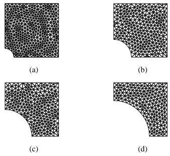
The problem is repeated with the application of the adaptive meshing technique. The plate with the hole size R/b
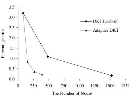
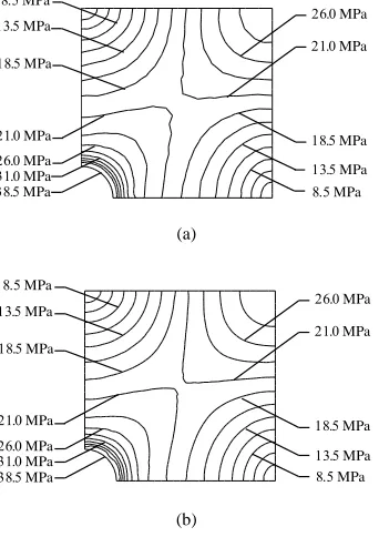
= 1/6 is considered again but a coarse mesh consisting of 84 nodes and 142 elements is used for the initial calculation as shown in Fig. 5(a). The Von Mises stresses obtained from this initial mesh solution are used as the key parameter to generate a new mesh. The new adaptive mesh, with 155 nodes and 268 elements, is shown in Fig. 5(b). The same process is applied to generate the second and third meshes. The second adaptive mesh with 267 nodes and 471 elements and the third adaptive mesh with 388 nodes and 694 elements are illustrated in Figs. 5(c) and 5(d), respectively. Small elements are clustered in the region of high stress gradients near the edge of the circular hole such that the solution accuracy of the problem will be increased. The finer mesh model with 1,521 nodes and 2,922 elements as shown in Fig. 6 is also analyzed. The percentage errors of the maximum transverse deflections from both methods are shown in Fig. 7. The results indicate that the adaptive meshing technique provides the same solution accuracy of the problem as the finer mesh but with fewer numbers of unknowns. The Von Mises stress contours obtained from the third adaptive mesh and the fine mesh are also shown in Figs. 8(a-b).
(a) (b)
(c) (d)
Fig. 5. DKT finite element meshes: (a) initial mesh, (b) 1st adaptive mesh, (c) 2nd adaptive mesh and (d) 3rd adaptive mesh.
Fig. 6. The fine DKT finite element model.
0.0 0.5 1.0 1.5 2.0 2.5 3.0 3.5
0 250 500 750 1000 1250 1500 1750 DKT (uniform)
Adaptive DKT
The Number of Nodes
P
er
ce
nt
age
e
rr
or
Fig. 7. Comparative percentage errors of the plate maximum transverse deflections obtained from the adaptive and uniform meshes.
θ (degree)
. MPa . MPa
. MPa
. MPa
. MPa
. MPa
. MPa . MPa . MPa . MPa
. MPa . MPa
(a)
. MPa . MPa
. MPa
. MPa
. MPa
. MPa
. MPa . MPa . MPa . MPa
. MPa . MPa
(b)
Fig. 8. Predicted Von Mises stress contours of the plate: (a) 3rd adaptive mesh and (b) fine mesh.
5.2 Plate attached with roof-like section subjected to vertical loading
To demonstrate the capability of the adaptive meshing technique for stress analysis of more complex plate structures, a plate attached with a roof-like section with the thickness of 5 mm subjected to vertical loading is considered. A problem statement of this example is presented in Fig. 9. The square plate is clamped along the edge x = 0 and subjected to the uniform vertical load along the opposite edge.
Fig. 9. Problem statement of a plate attached with roof-like section subjected to the uniform vertical load.
Due to the geometrical symmetry, the right half of the plate is analyzed. The first model to be analyzed is a fine mesh with 1,633 nodes and 3,100 elements as shown in Fig. 10(a). The Von Mises stress distribution obtained from the model is illustrated in Fig. 10(b). The calculation requires a great deal of computational time to get the results due to numerous unknowns.
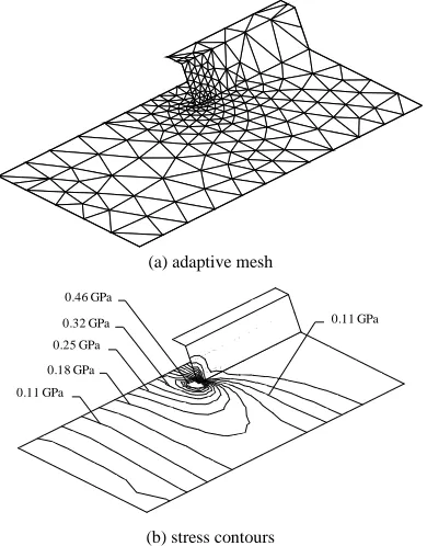
The adaptive meshing technique is now applied to the analysis. The initial unstructured coarse mesh consisted of 264 nodes and 458 elements as shown in Fig. 11(a) is analyzed first. The predicted Von Mises stress contours of the initial mesh are shown in Fig. 11(b). With these stresses, the new adaptive mesh with 237 nodes and 428 elements shown in Fig. 12(a) is constructed. Small elements are generated in the high stress regions at the corner of the intersection between the square plate and the roof-like section, while larger elements are generated in the other regions. The new refined mesh provides a more accurate and smoother stress distribution solution, as shown in Fig. 12(b). The figure indicates that the adaptive mesh provides the same accuracy as the fine mesh with fewer elements. The adaptive meshing technique can reduce much computational effort with the same solution accuracy instead of using fine mesh for the whole domain. The deflection of the adaptive mesh of the plate is also shown in Fig. 13.
(a) fine mesh
0.32 GPa 0.25 GPa 0.18 GPa 0.11 GPa
0.11 GPa 0.46 GPa
(b) stress contours
Fig. 10. The fine DKT finite element mesh and predicted Von Mises stress contours of the plate attached with roof-like section.
(a) initial mesh
E = 1.9×10¹¹ N/m2
ν = 0.3 thickness = 5 mm
16 cm 60o
8 cm
p = 2 kN/m
80 cm
80 cm 32 cm
x
y z
0.32 GPa 0.25 GPa 0.18 GPa 0.11 GPa
0.11 GPa
(b) stress contours
Fig. 11. Initial finite element mesh and predicted Von Mises stress contours of the plate attached with roof-like section.
(a) adaptive mesh
0.32 GPa 0.25 GPa 0.18 GPa 0.11 GPa
0.11 GPa 0.46 GPa
(b) stress contours
Fig. 12. Adaptive finite element mesh and predicted Von Mises stress contours of the plate attached with roof-like section.
D
ef
le
ct
ion
(m
)
0 0.05
-0.05
x
y
Fig. 13. Predicted deflection of the plate attached with roof-like section using adaptive finite element mesh.
5.3 Orthogonal intersection plate with rectangular hole subjected to vertical loading
Another example in analyzing built-up structures is considered. Such structure is a combination of two rectangular plates, 1×0.6 m and 1×0.4 m, that combine
orthogonally with a rectangular hole at the center. A problem statement of this example is denoted in Fig. 14. The plate structure has constant thickness of 1 cm. The plate is assumed to have the modulus of elasticity of 6.8×10¹⁰ N/m2 and the Poisson’s ratio of 0.33. The plate is clamped along the edge
y=0 and subjected to the uniform vertical load p=2,500 N/m along the opposite edge.
y z
x
1 m
0.6 m 0.4 m 0.2 m
0.1 m
0.3 m 0.4 m
p= 2,500 N/m
Fig. 14. Problem statement of the orthogonal intersection plate with rectangular hole subjected to vertical loading.
First, a fine finite element model is constructed as demonstrated in Fig. 15(a). The model consists of 1,739 nodes and 3,270 elements. The Von Mises stress distribution obtained from the model is shown in Fig. 15(b).
(a) fine mesh
25 MPa
35 MPa
50 MPa 15 MPa
30 MPa 40 MPa
(b) stress contours
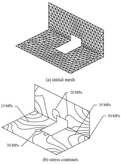
Next, the application of the adaptive meshing technique starts by constructing a coarse mesh (Fig. 16(a)) which consists of 460 nodes and 816 elements. The Von Mises stress distribution obtained from the initial mesh is shown in Fig. 16(b). The new adaptive mesh with 704 nodes and 1,279 elements shown in Fig. 17(a) is constructed according to the Von Mises stress obtained from the previous calculation. Small clustered elements are generated in the regions of high stress gradients to obtain higher solution accuracy around the corner of the hole and plate, while larger elements are generated in the other regions. Figure 17(b) shows the Von Mises stress contour obtained from the adaptive mesh demonstrating the advantage of the adaptive meshing technique (i.e., providing the same accuracy as the fine mesh but with fewer elements).
(a) initial mesh
20 MPa
35 MPa
50 MPa 15 MPa
30 MPa
(b) stress contours
Fig. 16. Initial finite element mesh and predicted Von Mises stress contours of the orthogonal intersection plate with rectangular hole.
(a) adaptive mesh
25 MPa
35 MPa
50 MPa 15 MPa
30 MPa
40 MPa
(b) stress contours
Fig. 17. Adaptive finite element mesh and predicted Von Mises stress contours of the orthogonal intersection plate with rectangular hole.
6.CONCLUSION
An adaptive meshing technique combined with the DKT finite element for plate bending analysis of built-up structures was presented. The DKT plate bending element has been combined with the adaptive meshing technique to improve the solution accuracy and to reduce the computational effort. The examples presented in this paper demonstrated that the adaptive meshing technique: (1) reduces modeling effort because a priori knowledge of the solution is not required; (2) provides improved solution accuracy by adapting the mesh to the physics of the solutions; (3) reduces the total number of elements used in the finite element modeling by automatically generating small elements in the regions with high solution gradients and large elements in the other regions.
REFERENCE
[1] Batoz, J. L., Zheng, C. L. and Hammadi, F. (2001). Formulation and Evaluation of New Triangular, Quadrilateral, Pentagonal and Hexagonal Discrete Kirchhoff Plate/Shell Elements, International Journal for Numerical Methods in Engineering, Vol. 52 (5-6), 615-630.
[2] Mackerle, J. (2002). Finite Element Linear and Nonlinear, Static and Dynamic Analysis of Structural Elements, an Addendum a Bibliography (1999-2002), Engineering Computations, Vol. 19 (5), 520-594. [3] Hrabok, M. M. and Hrudey, T. M. (1984). A Review and Catalogue of
Plate Bending Finite Elements, Computers and Structures, Vol. 19 (3), 479-495.
[4] Yang, H. T. Y., Saigal, S., Masud, A. and Kapania, R. K. (2000). A Survey of Recent Shell Finite Elements, International Journal for Numerical Methods in Engineering, Vol. 47 (1-3), 101-127.
[5] Gal, E. and Levy, R. (2006). Geometrically Nonlinear Analysis of Shell Structures Using a Flat Shell Finite Element, Archives of Computational Methods in Engineering, Vol. 13 (3), 331-388.
[6] Serpik, I. N. (2010). Development of a New Finite Element for Plate and Shell Analysis by Application of Generalized Approach to Patch Test, Finite Elements in Analysis and Design, Vol. 46 (11), 1017-1030. [7] Bernadou, M. (1996). Finite Element Methods for Thin Shell Problems,
1st Edn., John Wiley & Sons, New York, USA.
[8] Batoz, J. L., Bathe, K. J. and Ho, L. W. (1980). A Study of Three-node Triangular Plate Bending Elements, International Journal for Numerical Methods in Engineering, Vol. 15 (12), 1771-1812.
[9] Batoz, J. L. (1982). An Explicit Formulation for an Efficient Triangular Plate-bending Element, International Journal for Numerical Methods in Engineering, Vol. 18 (7), 1077-1089.
[11] Wanji, C. and Cheung, Y. K. (1999). Refined Non-conforming Triangular Elements for Analysis of Shell Structures, International Journal for Numerical Methods in Engineering, Vol. 46 (3), 433-455. [12] Paweenawat, A. and Dechaumphai, P. (2006). Nodeless Variables Finite
Element Method and Adaptive Meshing Technique for Viscous Flow Analysis, KSME International Journal, Vol. 20 (10), 1730-1740. [13] Limtrakarn, W. and Dechaumphai, P. (2004). Interaction of High-Speed
Compressible Viscous Flow and Structure by Adaptive Finite Element Method, KSME International Journal, Vol. 18 (10), 1837-1848. [14] Dechaumphai, P. (2010). Finite Element Method: Fundamentals and
Applications, 1st Edn., Alpha Science International, Oxford.
[15] Ugural, A. C. (1999). Stress in plates and shells, 2nd Edn., McGraw-Hill,
Singapore.
[16] Cook, R. D., Malkus, D. S., Plesha, M. E. and Witt, R. J. (2002). Concepts and applications of Finite Element Analysis, 4th Edn., John Wiley & Sons, New York.
[17] Jeyachandrabose, C., Kirkhope, J. and Babu, C. R. (1985). An Alternative Explicit Formulation for the DKT Plate-Bending Element, International Journal for Numerical Methods in Engineering, Vol. 21 (7), 1289-1293.
[18] Lo, C. C. and Leissa, A. W. (1967). Bending of Plates with Circular Holes, Acta Mechanica, Vol. 4 (1), 64-78.
[19] Klekiel, T. and Kołodziej, J. A. (2006). Trefftz method for large deflection of plates with application of evolutionary algorithms, Computer Assisted Mechanics and Engineering Sciences, Vol.13 (3), 407-416.
Pramote Dechaumphai received his B.S. degree in Industrial Engineering
from Khon-Kaen University, Thailand, in 1974, M.S. degree in Mechanical Engineering from Youngstown State University, USA in 1977, and Ph.D. in Mechanical Engineering from Old Dominion University, USA in 1982. He is currently a Professor of Mechanical Engineering at Chulalongkorn University, Bangkok, Thailand. His research interests are numerical methods, finite element method for thermal stress and computational fluid dynamics analysis.
Pichayen Bhothikhun received his B.S. and M.S. degrees in Mechanical