A Practical Graph Isomorphism Algorithm with
Vertex Canonical Labeling
Aimin Hou, Qingqi Zhong, Yurou Chen
School of Computer, Dongguan University of Technology, Dongguan 523808, China Email: {[email protected], [email protected], [email protected]}
Zhifeng Hao
Faculty of Computer, Guangdong University of Technology, Guangzhou 510006, China Email: [email protected]
Abstract—The vertex canonical labeling technique is one of the powerful methods in solving the graph isomorphism problem. However, some famous algorithms relied upon this technique are incomplete due to their non-zero probability of rejection. In this paper, we advance a new method of vertex canonical labeling and propose a complete graph isomorphism algorithm with depth-first backtracking. The time complexity of this algorithm is O(n^α) where n^α is the number of backtracking points and (h-1)/2≤α≤(h+1)/2 for h=logn in most cases. Finally, the proposed algorithm is compared with other researches on many types of graphs. The performance results validated that our algorithm is efficient for a wide variety of families of graphs.
Index Terms—canonical labeling; graph isomorphism; backtracking algorithm; completeness; time complexity
I. INTRODUCTION
A graph isomorphism is a bijective mapping between the vertices of two graphs that have the same number of vertices, identical labels, and an identical edge structure. Graph isomorphism is an important problem in graph theory and graph data application. So far no polynomial time algorithms [1] have been found for undirected graph isomorphism. Practical isomorphism algorithms may be roughly classified into two main categories.
The first category uses a direct approach. They take the two graphs to be compared based on some invariants, and try to find an isomorphism between them directly with a classical depth-first backtracking algorithm, possibly using heuristics to prune the search tree of possible mappings. This kind of algorithms [2-8] belongs to the Vertex Partition Refinement Algorithm.
The second category uses a different approach. They take a single graph G and compute some function C(G)
which returns a certificate (canonical labeling) of the graph, such that for two graphs G and H, C(G)=C(H) if
and only if G and H are isomorphic. Once the certificates
have been computed, comparing them is straightforward. This kind of algorithms [9-13, 16, 18-19] belongs to the Vertex Canonical Labeling Algorithm.
However, all of these vertex canonical labeling algorithms are incomplete. For the graphs that can be canonically labeled, they give quick positive or negative
answers. But for the graphs that cannot be canonically labeled, they answer “I do not know” (incomplete algorithms). Therefore, they have a non-zero probability of rejection and cannot work for all kinds of graphs even though they have polynomial time complexity.
In this paper, we advance a new method of vertex canonical labeling and propose a complete practical graph isomorphism algorithm with depth-first backtracking. This algorithm has a time complexity of O(n^α) where n^α is the number of backtracking points and (h-1)/2≤α ≤(h+1)/2 for h=logn in most cases.
By comparing the performance of four practical graph isomorphism algorithms, i.e., Nauty 2.2 [22], VF2 [5], our VPFA [8] and our VCLA proposed in this paper, on many types of graphs [23-24], we find that our VCLA is efficient for a wide variety of families of graphs.
The remainder of this paper is organized as follows. In Section II, we introduce some notations and properties presented in the literature. In Section III and IV, we investigate the new canonical labeling technique and the complete graph isomorphism algorithm, respectively. In Section V, we analyze our algorithm complexity. In Section VI, we obtain the test results on the performance comparison between our approach and other researches. Finally, we conclude the paper in Section VII.
II. PRELIMINARIES
This section offers a brief overview of canonical labeling methods. Canonical labeling of a graph refers to assigning a unique label to each vertex such that the labels are invariant under isomorphism. More formally, given a class ℵ of graphs which is closed under isomorphism, a canonical labeling algorithm assigns the numbers 1,…,n to the vertices of each graph in ℵ, having n vertices, in such a way that two graphs in ℵ are isomorphic if and only if the obtained labeled graphs coincide.
A. The First Category
The first category uses a function C(v) or C(G) which
returns a certificate (canonical labeling) of the vertex v or the graph G. For example, Babai [9-11] defines a binary
coded function C(v(i))=∑1≤j≤na(i, j)×2j and a(i, j)=1 if v(i) and v(j) are adjacent, and a(i, j)=0 otherwise. McKay [18] defines a function C(G, π) = max{G(v) | v∈X(G, π) and
max{Λ(G, π, v)}} where π is a partition of the vertex set V(G) of graph G, X(G, π) is the set of all terminal nodes
of the search tree T(G, π) (namely, the nodes are stable
vertex colorings), T(G, π) is the set of all partition nests,
and Λ(G, π, v) is a map of ℵ×[π]×[v]→Δ (any a linearly
ordered set). In other words, McKay’s method uses the automorphism group of the input graph to compute its canonical form.
B. The Second Category
The second category uses some an invariant as the label of a vertex v by sorting in lexicographic order. For example, Tomek and Gopal [12] use the degree neighborhood list of a vertex as the invariant and sort vertices in lexicographic order as the canonical label. The degree neighborhood of a vertex is a sorted list of the degrees of the vertex’s neighbors. Bollobás [13] uses the properties of the distance sequence of a vertex as the invariant. The distance sequence of a vertex v is the list {di(v), 1≤i≤n} where di(v) is the number of vertices at distance i from v. Emms et al. [20] use the continuous-time quantum walk as the invariant.
C. Canonical Labeling Algorithm
The following canonical labeling algorithm has been summarized for random graph isomorphism [9-13, 16, 18, 19].
1. Compute r = [3logn/log2].
2. Compute the degree of each vertex of the graph G.
3. Sort the vertices by their degree; call them v(1), ..., v(n). Denote by d(i) the degree of v(i): d(1)≥d(2)≥…≥d(n).
4. If d(i)=d(i+1) for some i∈{1, ...,r−1}, then G∉ℵ,
FAIL. Note: ℵ is the family of canonical labeled graphs. 5. Compute the canonical label of each vertex.
6. Sort the vertices by their canonical label in lexicographic order. Denote by C(i) the canonical label of v(i): C(1)≥C(2)≥…≥C(n).
7. If C(i)=C(i+1) for some i∈{1,...,r−1} or i∈{r,...,n}, then G∉ℵ, FAIL.
8. Label v(i) by C(i) for i∈{1, ...,n} in the sorted order. This labeling will be canonical, and G∈ℵ. END.
Obviously, the algorithm above is easy to test the isomorphism of random graphs with linear average time complexity. But it is hard to test the isomorphism of certain families of strongly regular graphs due to their non-zero probability of rejection. Namely, the Step 4 or 7 of the above algorithm holds for strongly regular graphs. D. Incompleteness
A naive algorithm has been presented in [9] that was able to canonically label almost all random graphs on n vertices in average linear time. In fact, it is shown there that the probability that a random graph on n vertices can
be canonically labeled with that algorithm is greater than 1−(1/n)1/7 (for sufficiently large n). Subsequently, Babai
and Kucera [10] improve this result obtaining a linear time canonical labeling algorithm with only exp(−cnlogn/loglogn) probability of failure.
In [11] Babai and Luks describe the known fast algorithm to compute canonical forms of general graphs in exp(n1/2+o(1)) time. The most powerful algorithm
currently available is McKay’s Nauty package [22] which is considered to be the first practical algorithm to employ the idea of Babai [9]. Despite its impressive performance in most cases, there are some families of graphs, which have very few automorphisms, but a high degree of regularity, that force it to run in exponential time [19] due to the construction of its canonical labeling.
E. VF2
In [5], Cordella advanced the famous VF2 algorithm. PROCEDURE Match(s)
INPUT: an intermediate state s; the initial state s0 has M(s0)=∅
OUTPUT: the mappings between the two graphs IF M(s) covers all the nodes of G2 THEN
OUTPUT M(s) ELSE
Compute the set P(s) of the pairs candidate for inclusion in M(s)
FOREACH (n, m)∈P(s) IF F(s, n, m) THEN
Compute the state s’ obtained by adding (n, m) to M(s) CALL Match(s’)
END IF
END FOREACH Restore data structures END IF
END PROCEDURE
The matching process can be suitably described by means of a State Space Representation (SSR). Each state s of the matching process can be associated to a partial mapping solution M(s), which contains only a subset of the components of the mapping function M. A partial mapping solution univocally identifies two subgraphs of
G1 and G2, say G1(s) and G2(s), obtained by selecting
from G1 and G2 only the nodes included in the
components of M(s), and the branches connecting them. F(s, n, m) is a boolean function (called feasibility function) that is used to prune the search tree. If its value is true, it is guaranteed that the state s’ obtained adding (n, m) to s is a partial isomorphism if s is. In order to evaluate F(s, n, m) the algorithm examines all the nodes connected to n and m; if such nodes are in the current partial mapping (i.e. they are in M1(s) and M2(s)), the algorithm checks if each branch from or to n has a corresponding branch from or to m and vice versa. Moreover, F will also prune some states that, albeit corresponding to an isomorphism between G1(s) and G2(s), would not lead to a complete matching solution.
F. VPFA
Algorithm: VPFA—Vertex Partition reFinement Algorithm
Step 1: Initialize the vertex match set VM(u)={v | v∈V(H)} for all vertex u∈V(G) and iteration step t=0.
Step 2: Compute an arbitrary predefined invariant for the graphs G and H, respectively.
Step 3: Sort the vertices by this invariant in lexicographic order.
Step 4: If the order of vertices of the graph G and H
are distinct and t=0, they are not isomorphic, FAIL. Step 5: Compute the partition set PG and PH decided by the invariant respectively.
Step 6: Computer the vertex match set VM(u)={ v | where u∈one cell of PG, v∈one cell of PH, u and v have the identical invariant value}.
Step 7: Compute the intersecting set of two successive vertex match sets in iterative processes. Update the all VM(u)s by its intersecting set.
Step 8: If there exist some an empty intersecting set and t=0, the graph G and H are not isomorphic, FAIL.
Otherwise, the current corresponding graphs are not isomorphic. Backtrack, set t=t-1. If t<0, the graph G and H are not isomorphic, FAIL. Otherwise, consider another
element of VM(u) in Step 9 of the previous iteration. Step 9: Select such a vertex u that VM(u) has the smallest size. Select arbitrarily one element v of VM(u), in which the vertex v has not been considered so far.
Step 10: Update the current corresponding graphs G
and H by deleting the u and v from G and H respectively.
Set t=t+1. Go to Step 2.
In our VPFA, an arbitrary predefined invariant is used to establish an initial partition of the vertices of the pair of original graphs G and H and to generate successive
partitions of the vertices of their subgraphs by deleting the corresponding vertices in an iterative process.
Two heuristic strategies are applied in the VPFA to shape the search tree of possible mappings. Strategy 1 chooses a vertex in the smallest cell of a partition in each iteration cycle. With this strategy, refinement realized by asserting a pair of vertices in the smallest cell may reduce the size of a large cell and hence reduce the breadth of the searching tree. Strategy 2 makes intersecting operation on two successive partitions obtained in two successive iteration cycles. With this strategy, a pair of corresponding vertices mapped in the previous iterations must be verified for consistency in the current iteration and hence reduce the depth of the searching tree.
III. NEW CANONICAL LABELING
Canonical labeling technique plays a key role in the structure of canonical labeling algorithm. In this section we introduce a new canonical labeling technique and discuss its quality.
A. New Canonical Labeling
We define a new canonical labeling based on probability list as follows. The computation of the label probabilities and the canonical labeling rely on the following notations.
Suppose there exist constants p1
1l, p112, p113, p21l, p212,
p2
13 where:
(I) for all x∈V, all (y, z)∈E where y∈V, z∈V: (i) max{| {(y, z) | (x, y)∈E; (x, z)∈E|} = p1
1l
(ii) max{| {(y, z) | (x, y)∈E; (x, z)∉E|} = p1
12 (1)
(iii) max{| {(y, z) | (x, y)∉E; (x, z)∉E|} = p1 13
(II) for all x∈V, all (y, z)∉E where y∈V, z∈V: (i) max{| {(y, z) | (x, y)∈E; (x, z)∈E|} = p2
1l
(ii) max{| {(y, z) | (x, y)∈E; (x, z)∉E|} = p2
12 (2)
(iii) max{| {(y, z) | (x, y)∉E; (x, z)∉E|} = p2 13
For a particular vertex x∈V, compute its constants px1 1l,
px1
12, px113, px21l, px212, px213 where:
(I) for all (y, z)∈E where y∈V, z∈V: (i) |{(y, z) | (x, y)∈E; (x, z)∈E|} = px1 1l
(ii) |{(y, z) | (x, y)∈E; (x, z)∉E|} = px1
12 (3)
(iii) |{(y, z) | (x, y)∉E; (x, z)∉E|} = px1 13
(II) for all (y, z)∉E where y∈V, z∈V: (i) |{(y, z) | (x, y)∈E; (x, z)∈E|} = px2
1l
(ii) |{(y, z) | (x, y)∈E; (x, z)∉E|} = px2
12 (4)
(iii) |{(y, z) | (x, y)∉E; (x, z)∉E|} = px2 13
For a particular vertex x∈V, compute its label probability Prob(x) as follow:
Prob(x)=∏1≤i≤2,1≤j≤3(pxi1j/pi1j) (5)
For a particular vertex x∈V, compute its label probability list Prob_list(x) as follow:
Prob_list(x)= (px1
1l/p11l, px112/p112, px113/p113, px21l/p21l,
px2
12/p212, px213/p213) (6)
Here, for all (pxi
1j/pi1j), if either pxi1j or pi1j equals 0,
(pxi
1j/pi1j) equals 1 where 1≤i≤2, 1≤j≤3.
For a particular vertex x∈V, compute its canonical labeling C(x) in lexicographically ordered as follow:
C(x)= a list (C(yl), … , C(yi)) where yj is the vertex adjacent to x (1≤j≤i) (7)
B. Quality
The quality of canonical labeling can be referred as the ability of distinguishing the distinct vertices under isomorphism. The more the distinct vertices have been distinguished, the high the quality of canonical labeling is. Of course, the technique of canonical labeling is an invariant under isomorphism in this sense.
In [8], we analyze the partition and refinement ability of some invariants, i.e. degree neighborhood of a vertex [12], shortest distance (similar to Bollobás’ method [13]) and exclusive-OR distance. The above Equations (1) to (4) are the basis of the exclusive-OR distance. For some families of graphs, the shortest distance behaviors better than the exclusive-OR distance does. Instead, for other families of graphs, the exclusive-OR distance behaviors better than the shortest distance does. Besides, the exclusive-OR distance behaviors always better than the degree neighborhood does. The conditions (i) and (ii) of Equations (3) and (4) are the basis of the Babai’s method [9]. McKay’s method [18] relying upon automorphism is too complicated to analyze in this paper.
IV. BACKTRACKING CANONICAL ALGORITHM
labeling algorithm, which overcomes the deficiencies found in Nauty 2.2-like algorithms and can deal with all classes of graphs.
A. Scheme of Our Algorithm
The scheme of our algorithm is to represent graph G
only once and reorder graph H with backtracking
operation. The basic idea is that each vertex of one of the graphs can be assigned one label out of a discrete set of possible labels that determines which vertex of the other graph it corresponds to. During the matching process, for each vertex there is a vector of the probabilities of each candidate label and for each vertex the label having the maximum probability list in lexicographically ordered is chosen. Initially, an arbitrary predefined invariant is computed in order to determine the graphs are non-isomorphic. Then, in successive iterations, the probability of each vertex is modified taking into account the label probabilities of the neighboring vertex which has been already labeled canonically, until the process converges to a fixed representation of graph H, or a maximum
number of backtracking iterations is reached.
Suppose the algorithm succeeds for G. If the algorithm
fails for H, the graphs are not isomorphic. If it succeeds
for H, sort the edges of both graphs lexicographically by
the labels of their vertices and compare the lists. If they are identical, the graphs are isomorphic. Otherwise the graphs are not isomorphic.
B. Our Algorithm
Algorithm: VCLA—Vertex Canonical Labeling Algorithm
Step 1: Compute an arbitrary predefined invariant for the graph G and H, respectively.
Step 2: Sort the vertices by this invariant in lexicographic order.
Step 3: If the order of vertices of the graph G and H
are distinct, they are not isomorphic, FAIL.
Step 4: Compute the constants p11l, p112, p113, p21l, p212,
p2
13 relying on the Equations (1) and (2), respectively.
Step 5: Compute the canonical labeling of graph G
without backtracks as follows.
Step 5.1: For all x∈V(G), compute its label probability
Prob(x) relying on the Equation (5).
Step 5.2: If there exists such a vertex x that its probability Prob(x) is unique, label x by C(x)=(1). Otherwise.
Step 5.3: If there exists such a vertex x that its probability list Prob_list(x) is unique, label x by C(x)=(1). Otherwise.
Step 5.4: Select an arbitrary vertex x with the highest probability list, label x by C(x)=(1).
Step 5.5: For all y∈V(G)-{x | x is the vertex labeled
canonically}, repeat Step 5.1 to 5.4 until each element of
V(G) has been labeled canonically, except that the set V
in the above Equations (3) and (4) is modified by the set of {x | x is the vertex labeled canonically} and C(y)=a list (C(xl), … ,C(xi)) where xj (1≤j≤i) is the vertex adjacent to
y and labeled canonically.
Step 6: Compute the canonical labeling of graph H that
is similar to the labeling process of graph G, except that
in Step 5.4 and 5.5 a backtracking operation is included for choosing another vertex with the same probability list in the next iteration.
Step 7: Whenever the algorithm succeeds for graph H,
sort the edges of both graphs lexicographically by the labels of their vertices and compare the lists. If they are identical, the graphs G and H are isomorphic. END.
Otherwise.
Step 8: Do some backtracking operations for the representation of graph H until no a backtracking
operation can be done. That is, all the possible choices have already been tried. In this case, the graphs G and H
are not isomorphic. FAIL.
V. COMPLEXITY ANALYSIS
In the following we analyze our algorithm complexity. Supposed that O(nk) time is required to compute the invariant value where k is a constant, at least for general graphs, the order of our algorithm cannot be less than nk. That is, for a pair of isomorphic or non-isomorphic graphs, the lower bound is O(1×nk).
The upper bound is not obvious at first glance. The amount of work required by the algorithm depends on the number of branches explored. To estimate the worst possible case, assume that the vertices are arranged in such a way that the algorithm will be required to investigate every choice at each level.
We will determine the upper bound with a reasonable method. Supposed that nα is the number of backtracking points, the upper bound will be O(nα).
Let h be the largest depth of search tree and C(t) smallest
be the selected cell at level t with the highest probability list. Thus there are at most |C(t)
smallest| branches from level
t. The maximum number of branches required is ∏0≤t≤h (|C(t)
smallest|). Note that this is a bound on the number of
branches which would be required to map a graph G onto
any other graph.
Due to the strategy of considering the set of neighborhoods labeled canonically of Step 5.5, the cell C(t)
smallest can be split by half in each iteration. In this case, ∏0≤t≤h(|C(t)smallest|)=(n/1)×(n/2)×(n/22)×(n/23)×…×(n/2h)
(where n/2h=1) = nh+1/20.5*h(h+1) =c×nα (where 1<c<n).
Therefore, nα≤nh+1/20.5*h(h+1)≤nα+1. Thus, (h-1)/2≤α≤
(h+1)/2 where h=logn. For the graphs discussed in the next section, α<3 in most cases, as the test results will show.
VI. TESTING RESULTS
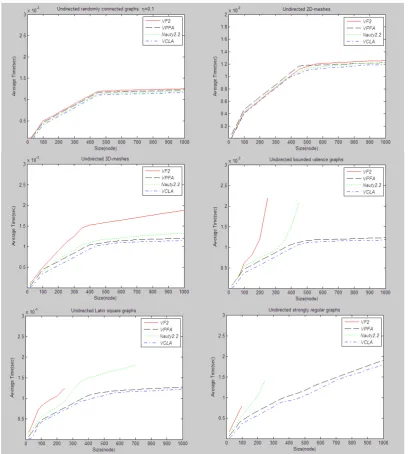
In this section we compare the performance of our algorithm VCLA with the two famous reference programs: Nauty 2,2 [22] and VF2 [5], as well as one of our previous work VPFA [8]. The four algorithms are implemented in the C language and the tests are carried out on a computer with Intel(R) Core(TM) i3-2350M Processor/2.3GHz.
graph database available at http://amalfi.dis.unina.it/ graph/, http://www.win.tue.nl/~aeb/graphs/Paulus.html.
The test results (see Figure 1) show that our algorithm VCLA yields the best results on the database. It is also more efficient than another algorithm of ours, VPFA, which takes polynomial time (that takes superpolynomial
time in the worst case) for graph isomorphism as discussed in [8]. It is not surprising that the invariant should be computed once at each step of VPFA, which will cost an O(nk) time.
.
Figure 1. Performance comparison of four algorithms.
In evaluating performance, it is important to distinguish between the performance of the implementation and the performance of the algorithm. The performance of the implementation is measured by the total time required for the program to process a pair of graphs. The performance of the backtracking algorithm will be measured by the number of branches required to process a pair of graphs.
Strongly regular graphs are known to be amongst the hardest graphs for isomorphism testing and many backtrackings should be made. Therefore, we will give
exhaustive explains for the performance of four programs on the strongly regular graphs in Table I and II.
Paulus [24] made a complete enumeration of the conference matrices of order 25 and the two-graphs of order 26. He found that up to isomorphism there are 15 strongly regular graphs with parameters v=25, k=12, λ=5, μ=6 (and spectrum 121 212 (-3)12), and 10 strongly regular
graphs with parameters v=26, k=10, λ=3, μ=4 (and spectrum 101 213 (-3)12).
regular graphs with parameters (25,12,5,6). The arrangement on combinations was introduced firstly by Schmidt [3] in his Table XII. Table II shows the actual number of branches and the depth of search tree on various combinations of strongly regular graphs with parameters (26,10,3,4).
Our algorithms VCLA and VPFA are competent to handle strongly regular graphs because the former considers the set of neighborhoods labeled canonically at each step while the latter chooses a vertex in the smallest cell of a partition at each step.
TABLE I:
TESTING RESULTS FOR STRONGLY REGULAR GRAPHS OF ORDER 25 Graph
1
Graph 2
Natuy 2.2 VF2 VPFA VCLA
# of Branches
Depth of Tree
# of Branches
Depth of Tree
# of Branches
Depth of Tree
# of Branches
Depth of Tree
P25.01 P25.02 3994 8 1997 8 728 7 860 5 P25.01 P25.03 3994 8 1902 8 728 7 860 5 P25.01 P25.04 4322 6 2060 6 794 5 1062 5 P25.01 P25.05 4326 7 2280 7 794 5 1062 5 P25.01 P25.06 3650 3 1722 3 650 2 650 2 P25.01 P25.07 4322 6 2362 6 794 5 1058 5 P25.01 P25.08 4658 6 2283 6 866 5 1262 5 P25.01 P25.09 3986 6 2133 6 710 4 854 4 P25.01 P25.10 3650 3 1614 3 650 2 650 2 P25.01 P25.11 4994 6 2357 6 890 4 1066 4 P25.01 P25.12 3650 3 1684 3 650 2 650 2 P25.01 P25.13 4010 8 1982 8 734 6 866 5 P25.01 P25.14 4658 6 2314 6 866 5 1062 5 P25.01 P25.15 3650 3 1679 3 650 2 650 2 P25.02 P25.01 3994 8 3994 8 728 7 858 5 P25.03 P25.01 3994 8 1564 8 726 6 856 5 P25.04 P25.06 3650 3 1762 3 650 2 650 2 P25.05 P25.07 4322 6 2102 6 794 5 1058 5 P25.06 P25.04 3706 6 1628 6 690 5 650 2 P25.08 P25.09 3986 6 1986 6 710 4 878 4 P25.08 P25.10 3650 3 1750 3 650 2 650 2 P25.09 P25.01 3986 6 1936 6 710 4 854 4 P25.10 P25.11 3794 4 1594 4 794 3 870 2 P25.13 P25.01 3994 8 1644 8 726 6 858 5 P25.15 P25.01 4270 7 2270 7 674 3 674 3
TABLE II:
TESTING RESULTS FOR STRONGLY REGULAR GRAPHS OF ORDER 26 Graph
1 Graph 2 # of Natuy 2.2 VF2 VPFA VCLA Branches
Depth of Tree
# of Branches
Depth of Tree
# of Branches
Depth of Tree
# of Branches
VII. CONCLUSIONS
In this paper we presented a practical vertex canonical labeling algorithm for graph isomorphism. This algorithm runs in O(n^α) time, where n^α is the number of backtracking points and (h-1)/2≤α≤(h+1)/2 for h=logn in most cases. Extensive experiments were carried out on many types of graphs, comparing this algorithm with the popular vertex partition refinement algorithm. The results show that our vertex canonical labeling algorithm is efficient for a wide variety of families of graphs.
Following are the significant findings of this paper: (I)A new method of canonical labeling of Equations (1) to (7). (II)Representation of canonical labeling for the first graph G in linear time (i.e. O(n^2), where n is the
number of vertices of graph G). (III)Iterative
representation of canonical labeling for the second graph
H with backtracking in superpolynomial time (i.e. O(n^α)
where α is a function of n.
Our future research will discuss the algorithm which hybridizes the vertex canonical labeling technique and the vertex partition refinement technique.
ACKNOWLEDGMENT
This work was supported by the National Natural Science Foundation of China (F020107) and the Natural Science Foundation of Guangdong Province, P.R.C. (9251009001000005).
REFERENCES
[1] B. Douglas. Introduction to Graph Theory. Pearson Education Asia Ltd., 2004, pp. 438-439.
[2] J.R. Ullmann, “An algorithm for subgraph isomorphism,” J. of the Association for Computer Machinery, vol. 23(1), 1976, pp.31-42.
[3] D.C. Schmidt and L.E. Druffel. “A fast backtracking algorithm to test directed graphs for isomorphism using distance matrices,” J. of the Association for Computer Machinery, vol. 23(3), 1976, pp.433-445.
[4] L.P. Cordella, P. Foggia, C. Sansone, et al. “Subgraph transformations for the inexact matching of attribute relational graphs,” IEEE Transactions on Pattern Analysis and Machinery Intelligence, vol. 26(10), 2004, pp.1367-1372.
[5] L.P. Cordella, P. Foggia, C. Sansone. “An improved algorithm for matching large graphs,” International Workshop on Graph-based Representation in Pattern Recognition, Ischia, Italy, 2001, pp. 149-159.
[6] M. Oliveria and F. Greve. “A new refinement procedure for graph isomorphism algorithms,” Proc. of the GRACO, 2005, pp. 373-379.
[7] X.X. Zou and Q. Dai. “A vertex refinement method for graph isomorphism,” J. of Software, vol. 18(2), 2007, pp.213-219.
[8] A.M. Hou, C.F. Hu, Z.F. Hao. “A general vertex partition refinement algorithm for graph isomorphism,” Advanced Materials Research, vol. 760-762, 2013, pp.1919-1924. [9] L. Babai, P. Erdös, S.M. Selkow. “Random graph
isomorphism,” SIAM J. of Computing, vol. 9, 1980, pp. 628-635.
[10]L. Babai and L. Kucera. “Canonical labeling of graphs in linear average time,” The 20th IEEE Symposium on Foundations of Computer Science, 1979, pp. 39-46.
[11]L. Babai and E.M. Luks. “Canonical labeling of graphs,” Proc. of the 15th Annual ACM Symposium on Theory of Computing, New York, USA, 1983, pp. 171-183.
[12]C. Tomek and P. Gopal. “Improved random graph isomorphism,” J. of Discrete Algorithm, vol. 6, 2008, pp.85-92.
[13]B. Bollobás. “Distinguishing vertices of random graphs,” Annals Discrete Math, Vol.13, 1982, pp.33-50.
[14]J.A. Fisteus, N.F. Garcia, L.S. Fernández, et al. “Hashing and canonical colour refinement,” J. of Computer and System Sciences, vol. 76(7), 2010, pp.663-685.
[15]Q.H. Zhou and Y. Li. “Isomorphic New Parallel Division Methods and Parallel Algorithms for Giant Matrix Transpose,” Journal of Computer, vol. 5(2), 2010, pp.169-177.
[16]M.I. Tikhomirov. “Fast canonical labeling of random subgraphs,” Doklady Math., vol. 87(2), 2013, pp.178-180. [17]J. Wu, L. Chen. “Mining frequent subgraph by incidence
matrix normalization,” Journal of Computer, vol. 3(10), 2008, pp.109-115.
[18]B.D. McKay. “Practical graph isomorphism,” Congressus Numberantium, vol. 30, 1981, pp.45-87.
[19]T. Miyazaki. “The complexity of McKay’s canonical labeling algorithm,” DIMACS Series in Discrete Mathematics and Theoretical Computer Science, vol. 28, 1997, pp.239-256.
[20]D. Emms, R.C. Wilson, E.R. Hancock. “Graph matching using the interference of continuous-time quantum walks,” Pattern Recognition, vol. 42(5), 2009, pp.985-1002. [21]X.G. Qiang, X.J. Yang, J.J. Wu, et al. “An enhanced
classical approach to graph isomorphism using continuous-time quantum walk,” J. of Physics A: Mathematical and Theoretical, vol. 45(4), 2012, pp.739-756.
[22]B.D. McKay. The Nauty Page. Computer Science Department, Australian National University. http://cs.anu.edu.au/~bdm/nauty/, 2004.
[23]The Graph Data, Collection of isomorphic graphs. http://amalfi.dis.unina.it/graph/.
[24]A.J.L. Paulus. “Conference matrices and graphs of order 26,” Technische Hogeschool Eindhoven, Report WSK, 1973, pp. 89-93.
Aimin Hou was born in Nanchang, Jiangxi, P.R.China, in June 19, 1963. He received B.S. degree and M.S. degree in Computer Science from Tianjin University, Tianjin, P.R.China in 1984 and 1989, respectively. He received Ph.D. degree in Computer Science and Application from South China University of Technology, Guangzhou, P.R.China in 2011.
He worked at Central South Design Institute of Building, Wuhan, Hubei, P.R. China from 1989 to 2003, employed in software development. He is currently an associate professor of computer science, Dongguan University of Technology, Guangdong Province, P.R. China. He has published more than 15 papers in journals including Artificial Intelligence, Advanced Materials Research, Journal of South China University of Technology, Journal of Computer Engineering and Application. In addition, he has published over 20 papers in refereed conferences. His research interest includes graph theory, data mining and intelligence computation.
and the Natural Science Foundation of Guangdong Province, China.
Qingqi Zhong was born in Dongguan, Guangdong Province, P.R.China, in August 15, 1984. He received B.S. degree in computer science from Dongguan University of Technology, P.R.China in 2007. He is currently a M.S. candidate in the School of Computer, Dongguan University of Technology, P.R.China.
Yurou Chen was born in Dongguan, Guangdong Province, P.R.China, in May 27, 1995. She is a sophomore in the School of Computer, Dongguan University of Technology, P.R.China.
Zhifeng Hao was born in Suzhou, Jiangsu, P.R.China, in December 09, 1968. He received B.S. degree in Mathematics from Sun Yat-Sen University, Guangzhou, P.R.China in 1990, and Ph.D. degree in Mathematics from Nanjing University, Nanjing, P.R.China in 1995.
From 1995 to 2008, he was a faculty member at Department of Mathematics, South China University
of Technology, Guangzhou, P.R.China, where he became a Professor in 2000. He is currently a full professor and Vice-President in Faculty of Computer, Guangdong University of Technology, Guangzhou, P.R.China. He has published more than 50 research papers in various refereed international journals. His research interest includes bioinformatics, kernel learning, nonlinear optimization, evolutionary algorithms and intelligence computation.