Multiple Operating Points Model-Based Control of
a Two-Wheeled Inverted Pendulum Mobile Robot
Mustapha Muhammad, Salinda Buyamin
*, M. N. Ahmad, S. W. Nawawi and A. A. Bature
Faculty of Electrical Engineering, Universiti Teknologi Malaysia, 81310 UTM Skudai, Johor Malaysia Email: [email protected]
Abstract – Literature review shows that, most of the linear controllers proposed for control of a Two-Wheeled Inverted Pendulum (TWIP) mobile robot are based on dynamic models that are linearized around a single operating point. Thus, this paper presents the controller design for a TWIP mobile robot based on its multiple operating point linearized model. The nonlinear dynamical equations of motion of the TWIP mobile robot were firstly obtained. The nonlinear equations were then linearized around different operating points resulting in a number of linear models with each represented a local region of the original nonlinear system. Based on the multiple operating points linearized models a state feedback control scheme was proposed using pole placement technique for balancing and tracking control of the TWIP mobile robot. The performance of the proposed controller investigated in terms of reference command tracking, parameter variation and external disturbance rejection via simulations. The simulation result shows the effectiveness of the proposed control scheme.
Index Term
--
Multiple Operating Points Linearized Model, State Feedback tracking Control, Two-Wheeled Inverted Pendulum (TWIP)NOMENCLATURE i
A
- System matricesi
B
- Input matrices)
(
t
x
-State vector)
(
t
u
-Input vector)
(
t
r
- Referenceinput vector)
(
t
z
n -Premise variables)
(
x
m
i -Selector1
- Wheel 1 torque2
- Wheel 2 torquei M
C - Controllability matrices
i M
O - Observability matrices
n
- Undamped natural frequency
- Damping ratios
t
- Settling timeM - Percentage overshoot
Ki - Controller gain matrices
Ni - Reference input scaling factor matrices
0
- Initial tilt angled
- Desired tilt angle0
- Initial orientation angled
- Desired orientation angle0
v
- Initial velocityd
v
- Desired velocityI. INTRODUCTION
A two wheeled inverted pendulum (TWIP) mobile robot is a three-degrees-of-freedom under-actuated mechanical system with highly nonlinear dynamics. This makes it a perfect test-bed for various control algorithms ranging from conventional theoretical control algorithms to intelligent control algorithms. In recent years, various control methods have been reported in literature for controlling the TWIP mobile robot. In the early work by Ha and Yuta [1], a linear state feedback and feed forward controller was designed and implemented for the posture and velocity control of the TWIP mobile robot. Grasser et al [2] proposed a linear state feedback controller based on pole placement technique for the robot. In [3] Nawawi et al a TWIP mobile robot was developed and stabilized using pole placement controller. Kim et al [4] investigated the exact dynamics of the TWIP, and developed a linear quadratic regulator (LQR) controller for balancing the robot. Fiacchini et al [5] proposed linear and nonlinear controllers for stabilizing a personal pendulum vehicle. In Seo et al [6] the performance of the two wheeled inverted pendulum on tilted road was investigated, and an LQR controller was proposed for the system. Nasir et al [7] compare the performance of LQR and PID in stabilizing two-wheeled balancing robot. In Jones and Stol [8], the performance of the two wheeled mobile robot in low-traction environment investigated by designing an LQR controller based on linearized model of the robot which includes wheel slip effects. Pathak et al [9] proposed velocity and position controllers for the TWIP robot via partial feedback linearization. In Li and Luo [10] an adaptive controller was proposed for the TWIP system which deals with model uncertainties. Huang et al [11] proposed three fuzzy controllers based on Takagi-Sugeno and Mamdani architectures for the balancing, traveling and steering of the TWIP mobile robot. Kausar et al [12], investigated the effect of terrain inclination on the performance and stability region of a two-wheeled mobile robot. In Muhammad et al [13] compare the performance of a partial feedback linearization and an LQR controller in balancing and velocity tracking control of the TWIP mobile robot.
International Journal of Mechanical & Mechatronics Engineering IJMME-IJENS Vol:13 No:05 2
137905-4848-IJMME-IJENS © October 2013 IJENS model of the TWIP mobile robot. The nonlinear dynamical
equations of motion of the TWIP mobile robot are linearized around different operating points, resulting in a number of linear models with each represented a local region of the original nonlinear system. Based on the multiple operating point linearized models a linear controller is designed using pole placement technique. The performance and robustness of the proposed controller are investigated via simulations.
The rest of the paper is organized as follows: Section two presents the mathematical of the TWIP, whereas section three presents the proposed controller design, in section four the Simulation results are presented and finally the conclusion is made in section five.
II. SCOPEANDLIMITATIONSOFTHEWORK
This research work was planned to cover:
• Development of multiple operating points linearized model of the TWIP mobile robot from its nonlinear dynamical model.
• Design of a new state feedback tracking controller based on the multiple operating points model of the TWIP mobile robot.
• Design of a conventional state feedback tracking controller based on a single operating point model of the TWIP mobile robot.
• Investigation of the balancing and tracking performances of the proposed controller via simulations
• Investigating the robustness of the proposed controller via simulations
• Comparative assessment between the proposed controller and a conventional linear controller in terms of robustness.
III. TWIPMOBILE ROBOT MODELING
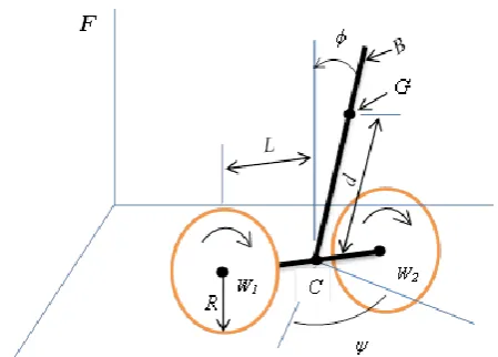
The model considered in this paper is based on the TWIP mobile robot presented by Nawawi et.al [14, 15]. The free body diagram of the TWIP mobile robot is shown in fig. 1. It is described based on the variables and parameters in table I
Fig. 1. Free body diagram of the TWIP with the system coordinate
TABLE I
TWIP MOBILE ROBOT PARAMETERS
Symbol Parameter/Variables Value Unit
mB mass of the main body of the TWIP 15 kg
mW mass of each wheel 0.42 kg
L half of the distance between the wheels 0.20 m
R radius of each wheel 0.106 m
I2 the moment of inertia of the body about n2 direction 0.63 kgm
2
I3 the moment of inertia of the body about n3 direction 1.12 kgm
2
G gravitational acceleration 9.81 m/s2
D distance between the center of the wheels axis C and the center of gravity G
0.212 m
Φ pendulum tilt angle rad
Ψ yaw angle (orientation of the robot) rad
X TWIP position m
III.1. Mathematical Modeling
The dynamical equations of the TWIP are derived using Kane’s method based on the assumption that the wheels of the robot always stay in contact with the ground and the wheels do not slip.
The forces exerted on the robot are assumed to be the torques between the wheels and body generated by the driving motors and the gravitational force at the center of the main body and that at the center of the wheels [16].
3
2 2 2 2 3 3
cos
I d m m m d m x B B W B B B B
3 2 2 2 2 3cos m m m d I
d
mB W B B
23 2 2 2 2 3 2 3 cos sin
I d m m m d m d m I d m B B W B B B
1 2
3 2 2 2 2 3 2 3 cos
cos
I d m m m d m R I d m dR m B B W B B B (1)
2 2 2 2 2 2 sin 2 1 3 cos sin I d m R L m d m B WB
2 1 2 2 2 2 2 sin 2 1 3 I d m R L m R L B W (2)
23 2 2 2 2 2 3 cos cos sin 3 I d m m m d m d m m B B W B B W
3 2 2 2 2 3 cos sin 3 I d m m m d m gd m m m B B W B B B W
2 3 2 2 2 2 2 2 3 cos cos sin
I d m m m d m d m B B W B B
1 2
3 2 2 2 2 3 cos cos
3
I d m m m d m R d m m m R B B W B B B W (3)
cos 2.619
cos sin 81 . 9 619 . 2 cos sin 4583 . 0 cos 25 . 0 2 2 2 2
x
2
1 2
2 2 619 . 2 cos 2095 . 0 cos 1143 . 0 619 . 2 cos sin 4583 .
0
(4)
2
2
1 2
6424 . 0 sin 3657 . 0 6424 . 0 sin cos
sin
(5)
cos 2.619
sin 0571 . 56 619 . 2 cos cos sin 4286 . 0 2 2
2
2
1 2
2 2 619 . 2 cos 6531 . 0 cos 4571 . 0 619 . 2 cos cos
sin
(6)
22 2 8849 . 2 cos sin 5642 . 0 8849 . 2 cos cos sin 81 . 9
x
2
1 2
8849 . 2 cos 6738 . 1 cos 3145 .
0
(7)
2
1 2
0128 . 1 sin 7987 .
2
(8)
22 2 8849 . 2 cos cos sin 8849 . 2 cos sin 1606 . 50
2
1 2
8849
.
2
cos
6079
.
1
cos
9667
.
2
(9)III.2. Multiple Operating Points Linearization
The nonlinear model of the TWIP mobile robot will be linearized around different operation points resulting in a number of linear models with each represented a local region of the original nonlinear system. The resulting linear models will then be used for the proposed controller design.
From the dynamical equations (7) and (9), it can be observed that the state variables that make the system
nonlinear are
and
. From expert knowledge [18]
0 2
and
0 6
. The following operating points were chosen for the tilt angle
: 0, 18, 9, 6, 29,18 5 ,
3
.
Based on the selected operating points the following 14 linear models are formulated:
Odd models 1-14: IF
is about i18 AND
is about 0, THENx
(
t
)
A
2i1x
(
t
)
B
2i1u
(
t
)
.i
0
,
1
,...
6
)
(
)
(
t
Cx
t
y
(10)
Even models 1-14:IF
is about i18 AND
is about 6,THEN
x
(
t
)
A
2(i1)x
(
t
)
B
2(i1)u
(
t
)
.i
0
,
1
,...
6
.y
(
t
)
Cx
(
t
)
(11)where:
T
]
[
)
(
t
x
x
x
T
]
[
)
(
t
1
2International Journal of Mechanical & Mechatronics Engineering IJMME-IJENS Vol:13 No:05 4
137905-4848-IJMME-IJENS © October 2013 IJENS
0 0643 . 26 0 0 0 0 1 0 0 0 0 0 0 0 0 0 0 0 0 0 1 0 0 0 0 02 . 5 0 0 0 0 0 0 0 0 1 0 3 A 5358 . 0 0643 . 26 0 0 0 0 1 0 0 0 0 0 0 0 0 0 0 0 0 0 1 0 0 0 3069 . 0 02 . 5 0 0 0 0 0 0 0 0 1 0 4 A 0 5483 . 24 0 0 0 0 1 0 0 0 0 0 0 0 0 0 0 0 0 0 1 0 0 0 0 5114 . 4 0 0 0 0 0 0 0 0 1 0 5 A 9632 . 0 5483 . 24 0 0 0 0 1 0 0 0 0 0 0 0 0 0 0 0 0 0 1 0 0 0 5784 . 0 5114 . 4 0 0 0 0 0 0 0 0 1 0 6 A 0 4366 . 22 0 0 0 0 1 0 0 0 0 0 0 0 0 0 0 0 0 0 1 0 0 0 0 8001 . 3 0 0 0 0 0 0 0 0 1 0 7 A 217 . 1 4366 . 22 0 0 0 0 1 0 0 0 0 0 0 0 0 0 0 0 0 0 1 0 0 0 7929 . 0 8001 . 3 0 0 0 0 0 0 0 0 1 0 8 A 0 0978 . 20 0 0 0 0 1 0 0 0 0 0 0 0 0 0 0 0 0 0 1 0 0 0 0 011 . 3 0 0 0 0 0 0 0 0 1 0 9 A 2856 . 1 0978 . 20 0 0 0 0 1 0 0 0 0 0 0 0 0 0 0 0 0 0 1 0 0 0 9469 . 0 011 . 3 0 0 0 0 0 0 0 0 1 0 10 A 0 8138 . 17 0 0 0 0 1 0 0 0 0 0 0 0 0 0 0 0 0 0 1 0 0 0 0 2394 . 2 0 0 0 0 0 0 0 0 1 0 11 A 1953 . 1 8138 . 17 0 0 0 0 1 0 0 0 0 0 0 0 0 0 0 0 0 0 1 0 0 0 0492 . 1 2394 . 2 0 0 0 0 0 0 0 0 1 0 12 A 0 7435 . 15 0 0 0 0 1 0 0 0 0 0 0 0 0 0 0 0 0 0 1 0 0 0 0 5395 . 1 0 0 0 0 0 0 0 0 1 0 13 A 986 . 0 7435 . 15 0 0 0 0 1 0 0 0 0 0 0 0 0 0 0 0 0 0 1 0 0 0 1126 . 1 5395 . 1 0 0 0 0 0 0 0 0 1 0 14 A T 4270 . 2 0 7633 . 2 0 0549 . 1 0 4270 . 2 0 7633 . 2 0 0549 . 1 0 2 1 B B T 3652 . 2 0 6834 . 2 0 0357 . 1 0 3652 . 2 0 6834 . 2 0 0357 . 1 0 4 3 B B T 1958 . 2 0 4772 . 2 0 9840 . 0 0 1958 . 2 0 4772 . 2 0 9840 . 0 0 6 5 B B T 9566 . 1 0 2163 . 2 0 9116 . 0 0 9566 . 1 0 2163 . 2 0 9116 . 0 0 8 7 B B T 6886 . 1 0 9627 . 1 0 8332 . 0 0 6886 . 1 0 9627 . 1 0 8332 . 0 0 10 9 B B T 6295 . 1 0 7496 . 1 0 7290 . 0 0 6295 . 1 0 7496 . 1 0 7290 . 0 0 12 11 B B T 1732 . 1 0 5876 . 1 0 6949 . 0 0 1732 . 1 0 5876 . 1 0 6949 . 0 0 14 13 B B 1 0 0 0 0 0 1 0 0 0 0 0 1 0 0 0 0 0 1 0 0 0 0 0 1 C
IV. CONTROL OF THE TWIPMOBILE ROBOT Based on the dynamic model obtained in the previous section two controllers are designed. The first controller is the proposed controller which is a state feedback tracking controller designed based on the multiple operating points linearized models, while the second controller is a conventional state feedback tracking controller, which is designed based on a single operating point linearized model of the TWIP mobile robot.
IV.1. Proposed Controller
The proposed controller is a state feedback tracking controller which is based on the multiple operating points linearized models. Fig. 2 shows the block diagram of a proposed state feedback tracking control system, where
)
(
t
x
is the state vector,u
(
t
)
is the control input vector,)
(
t
r
is the reference input vector andy
(
t
)
is the output vector.The proposed controller selects one set of the gains (Ki
i
N ) at a time based on the operating point at which the plant operate at that particular time, if the operating point changes then the controller select another set of gains which corresponds to the new operating point. From fig. 2 the linearized model of system around a particular operating point can be represented by the following state equation:
)
(
)
(
)
(
t
A
x
t
B
u
t
x
i
i (12)Also from fig. 2 the proposed control law can also be written as:
t
K
x
t
N
r
t
u
i
i (13)where
K
i andN
i are the controller gain and scaling factormatrices respectively, which depends on the operating point of the plant at a particular time.
Substituting the control law (13) in to the state equation (12) yields:
(
)
(
)
)
(
t
A
B
K
x
t
B
N
r
t
As steady state:
0
)
(
t
x
(15)ss
x
t
x
(
)
(16)The control goal here is make the system states
x
(
t
)
tracks the reference inputs
r
(
t
)
at steady state, that isss
x
t
r
(
)
(17)Substituting (15)-(17) in (14) yields:
A
i
B
iK
i
x
ss
B
iN
ix
ss
0
(18)Hence,
i i i
i
i
N
A
B
K
B
(19)Pre multiplying both sides of (19) by T
B yields:
i i i
i i i
i
B
N
B
A
B
K
B
T
T
(20)Pre and post multiplying both sides of (20) by
BiTBi
1yields:
i i
i
i i i
i
B
B
B
A
B
K
N
T 1 T
(21)Fig. 2.Proposed state tracking feedback control system The controllability and observability of the system at all
the operating points were checked using MATLAB based on equations (22) and (23) and found to be completely controllable and observable [19].
i i i i i i i i i i i
i
M B AB A B A B A B A B
C 2 3 4 5 i1,2,...,14 (22)
Ti i i i i i
M C CA CA CA CA CA
O 2 3 4 5
14 ,..., 2 , 1
i (23)
The proposed controller is designed based on the 14 linear models of the TWIP mobile robot obtained in the previous section using dominant pole pair based on the specifications of percentage overshoot of approximately 10% and settling time of less than 10 seconds for the pendulum tilt angle.
The closed loop poles are to be placed at s = pi
(i=1,2,….6) where p1and p2 are the dominant poles, which
are determine based on the specifications. The general second order system is given by:
2 2
2
2
)
(
n n n
s
s
s
G
(24)From the specification on percentage overshoot, the damping ratio
may be computed using [20]:%
10
%
100
2
1
e
M
(25)From the specification of settling time, the undamped
natural frequency
n may be computed using [20]:10
4
n st
(26)From (17) and (18)
and
n are obtained as 0.4559International Journal of Mechanical & Mechatronics Engineering IJMME-IJENS Vol:13 No:05 6
137905-4848-IJMME-IJENS © October 2013 IJENS poles are obtained using (24) as p1 =-0.4000 + 0.5458i and
p2 =-0.4000 - 0.5458i respectively. The other poles are
located far to the left of the dominant poles as p3 =-4, p4
=-4, p5 =-8p6 =-8. Based on these selected poles locations
the controller gain matrices are obtained as:
3.0746 14.3532 2.1713 5.7902 1.0068 0.4744 3.0746 14.3532 2.1713 -5.7902 -1.0068 0.4744 1 K 2.9521 10.3608 2.1713 5.7902 0.7249 0.3416 2.9521 10.3608 2.1713 -5.7902 -0.7249 0.3416 2 K 3.1561 14.6131 2.2360 5.9626 1.0281 0.4844 3.1561 14.6131 2.2360 -5.9626 -1.0281 0.4844 3 K 3.0405 14.5391 2.2360 5.9626 1.0227 0.4844 3.0405 14.5391 2.2360 -5.9626 -1.0227 0.4844 4 K 3.4036 15.3971 2.4221 6.4589 1.0911 0.5141 3.4036 15.3971 2.4221 -6.4589 -1.0911 0.5141 5 K 3.1791 15.2387 2.4221 6.4589 1.0794 0.5141 3.1791 15.2387 2.4221 -6.4589 -1.0794 0.5141 6 K 3.8274 16.7434 2.7072 7.2192 1.1943 0.5627 3.8274 16.7434 2.7072 -7.2192 -1.1943 0.5627 7 K 3.5075 16.4780 2.7072 7.2192 1.1752 0.5627 3.5075 16.4780 2.7072 -7.2192 -1.1752 0.5627 8 K 4.4480 18.7145 3.0570 8.1520 1.3332 0.6282 4.4480 18.7145 3.0570 -8.1520 -1.3332 0.6282 9 K 4.0533 18.3066 3.0570 8.1520 1.3048 0.6282 4.0533 18.3066 3.0570 -8.1520 -1.3048 0.6282 10 K 4.6612 18.7168 3.4294 9.1449 1.5749 0.7421 4.6612 18.7168 3.4294 -9.1449 -1.5749 0.7421 11 K 4.2663 17.9710 3.4294 9.1449 1.5146 0.7421 4.2663 17.9710 3.4294 -9.1449 -1.5146 0.7421 12 K 6.4633 25.1091 3.7793 10.0781 1.7021 0.8020 6.4633 25.1091 3.7793 -10.0781 -1.7021 0.8020 13 K 6.0109 24.2382 3.7793 10.0781 1.6477 0.8020 6.0109 24.2382 3.7793 -10.0781 -1.6477 0.8020 14 K
Using equation (21) the scaling factor matrices are computed as: 3.0746 9.3500 2.1713 5.7902 1.0068 0.4744 3.0746 9.3500 2.1713 -5.7902 -1.0068 0.4744 1 N 2.9521 9.4786 2.1713 5.7902 0.7249 0.3416 2.9521 9.4786 2.1713 -5.7902 -0.7249 0.3416 2 N 3.1561 9.5997 2.2360 5.9626 1.0281 0.4844 3.1561 9.5997 2.2360 -5.9626 -1.0281 0.4844 3 N 3.0405 9.5258 2.2360 5.9626 1.0227 0.4844 3.0405 9.5258 2.2360 -5.9626 -1.0227 0.4844 4 N 3.4036 10.3587 2.4221 6.4589 1.0911 0.5141 3.4036 10.3587 2.4221 -6.4589 -1.0911 0.5141 5 N 3.1791 10.2003 2.4221 6.4589 1.0794 0.5141 3.1791 10.2003 2.4221 -6.4589 -1.0794 0.5141 6 N 3.8274 11.6607 2.7072 7.2192 1.1943 0.5627 3.8274 11.6607 2.7072 -7.2192 -1.1943 0.5627 7 N 3.8406 11.3953 2.7072 7.2192 1.1752 0.5627 3.8406 11.3953 2.7072 -7.2192 -1.1752 0.5627 8 N 4.4480 13.5749 3.0570 8.1520 1.3332 0.6282 4.4480 13.5749 3.0570 -8.1520 -1.3332 0.6282 9 N 4.4707 13.1670 3.0570 8.1520 1.3048 0.6282 4.4707 13.1670 3.0570 -8.1520 -1.3048 0.6282 10 N 4.6612 13.9623 3.4294 9.1449 1.5749 0.7421 4.6612 13.9623 3.4294 -9.1449 -1.5749 0.7421 11 N 4.6909 13.2164 3.4294 9.1449 1.5146 0.7421 4.6909 13.2164 3.4294 -9.1449 -1.5146 0.7421 12 N 6.4633 19.8544 3.7793 10.0781 1.7021 0.8020 6.4633 19.8544 3.7793 -10.0781 -1.7021 0.8020 13 N 6.5299 18.9834 3.7793 10.0781 1.6477 0.8020 6.5299 18.9834 3.7793 -10.0781 -1.6477 0.8020 14 N
IV.2. Conventional Controller
This controller is a state feedback tracking controller which is designed based on the single operating point linearized model of the TWIP mobile robot.
The nonlinear of the TWIP mobile robot in (4)-(6) was linearized based on the following assumptions: 0, 0,
sin , cos1; hence the linearized model is represented in state space as follows:
) ( ) ( )
(t Axt But
x (27)
where:
T ] [
)
(t x x
x
T
]
[
)
(
t
1
2
0 6118 . 26 0 0 0 0
1 0 0 0 0 0
0 0 0 0 0 0
0 0 1 0 0 0
0 2045 . 5 0 0 0 0
0 0 0 0 1 0
A
4270 . 2 4270 . 2
0 0
7633 . 2 7633 . 2
0 0
0549 . 1 0549 . 1
0 0
B
Using the same procedure as in the previous section the state feedback tracking control law based the single operating point linearized model in (27) can be written as:
t
Kx
t
Nr
t
u
(28)The scaling factor matrix can also be derived as:
B
B
B
A
BK
N
T 1 T
(29)Using the specifications as in the previous section, the controller gain and scaling factor matrices are respectively computed as:
3.0746 14.3532 2.1713
5.7902 1.0068 0.4744
3.0746 14.3532 2.1713
-5.7902 -1.0068 0.4744
K
3.0746 9.3500 2.1713
5.7902 1.0068
0.4744
3.0746 9.3500 2.1713 -5.7902 -1.0068 0.4744
N
V. SIMULATION
The effectiveness and robustness of the proposed control scheme was investigated via simulations in Simulink. The simulation results are compared with those from a conventional linear controller. The performance of the controller was investigated in terms of reference command tracking, parameter variations and external disturbance rejection.
V.1. Reference command Tracking
The simulation was carried out with the desired velocity
vd =5m/s, the desired orientation angle ψd = π/18 rad,
desired tilt angle ϕd =0, and the initial conditions of velocity,
tilt angle and orientation angle as 0, π/6 rad and 0
respectively. Fig. 3 through 7 shows the simulation results. From fig. 3 it can be seen that the two controllers balanced the robot, both controllers settled the tilt angle in about 8.5 seconds, with an overshoot of 12.8%. Fig. 4 shows the velocity tracking response for the two controllers, both controllers settled in about 10.5 seconds, with an overshoot of about 25.9%. Both controllers’ tracks the reference orientation as shown in fig. 5, both controllers settled the orientation angle in about 1.5 seconds, with an overshoot of 0%. Figures 6 and 7 shows the control inputs for wheel 1 and wheel 2 required for the two controllers, from the result it can be seen that the proposed controller require slightly higher starting torque compare to the conventional controller under this condition.
0 2 4 6 8 10 12 14 16 18 20
-0.1 0 0.1 0.2 0.3 0.4 0.5 0.6
Time (s)
T
il
t
an
g
le
(
ra
d
)
Proposed Controller Conventional Controler
Fig. 3. Tilt angle tracking response
0 2 4 6 8 10 12 14 16 18 20
0 1 2 3 4 5 6 7
Time (s)
V
el
o
ci
ty
(
m
/s
)
Proposed Controller Conventional Controler
Fig. 4. Velocity tracking response
0 2 4 6 8 10 12 14 16 18 20
0 0.02 0.04 0.06 0.08 0.1 0.12 0.14 0.16 0.18
Time (s)
O
ri
en
ta
ti
o
n
(
ra
d
)
Proposed Controller Conventional Controler
Fig. 5. Robot Orientation tracking response
0 2 4 6 8 10 12 14 16 18 20
-4.5 -4 -3.5 -3 -2.5 -2 -1.5 -1 -0.5 0 0.5
Time (s)
T
o
rq
u
e
(N
m
)
Proposed Controller Conventional Controler
International Journal of Mechanical & Mechatronics Engineering IJMME-IJENS Vol:13 No:05 8
137905-4848-IJMME-IJENS © October 2013 IJENS
0 2 4 6 8 10 12 14 16 18 20
-3.5 -3 -2.5 -2 -1.5 -1 -0.5 0 0.5
Time (s)
T
o
rq
u
e
(N
m
)
Proposed Controller Conventional Controler
Fig. 7. Wheel 2 control input
V.2. Effect of parameters variation
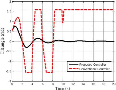
The performance of the two proposed controller was also compared with that of the conventional controller due to parameters variation under step command. Firstly the mass of the robot main body was doubled. The mass of the main body is directly proportional to the inertia of the main body; hence if the mass doubled, the inertia will also double. Therefore the simulation was carried out with both mass and inertia of the main body of the robot doubled. Fig. 8 shows the simulation result, which shows that the conventional controller fails to balance the robot while the proposed controller balance the TWIP mobile robot with a settling time of less than 14 seconds.
0 2 4 6 8 10 12 14 16 18 20
-2 -1.5 -1 -0.5 0 0.5 1 1.5 2
Time (s)
T
il
t
an
g
le
(
ra
d
)
Proposed Controller Conventional Controler
Fig. 8. Tilt angle response with mass and inertia doubled
V.3. Effect of External Disturbance
The pendulum is disturbed by an external force of 30N
while the robot is in motion, with
0
6,
d
18,s
m
v
d
5
/
. Fig. 9 shows the simulation result, which shows that the conventional controller failed to balance the robot, while the proposed controller is able to with stand the disturbance.0 5 10 15 20 25 30 35 40 45 50
-2 -1.5 -1 -0.5 0 0.5 1 1.5 2
Time (s)
T
il
t
an
g
le
(
ra
d
)
Proposed Controller Conventional Controler
Fig. 9. Tilt angle response due to external disturbance
VI. CONCLUSION
The nonlinear dynamical equations of motion of the TWIP mobile robot were first obtained. The dynamical equations were then linearized around multiple operating points. A linear controller using pole placement technique was then proposed based on the multiple operating points’ linearized models. A conventional linear controller was also designed based on a single operating point linearized model of the TWIP mobile robot. The performance of the proposed controller was compared with that of the convention linear controller in terms of reference command tracking, effects of parameter variation and effects of external disturbance via simulations. The simulations results show that, both controllers balanced the robot, and track the reference velocity and reference orientation; however the conventional controller failed to balance the robot under the effect of parameters variation and external disturbance, while the proposed controller was able to balance the robot under the effect of parameter variation and in the presence of disturbance. In Further work the performance proposed controller obtained through simulations can be verified experimentally on the actual TWIP mobile robot.
ACKNOWLEDGEMENTS
Special thanks Universiti Teknologi Malaysia for the facilities and infrastructure and Bayero University, Kano, Nigeria for the sponsorship.
REFERENCES
[1] Y. Ha, and S. Yuta, Trajectory tracking control for navigation of the inverse pendulum type self-contained mobile robot, Robotics and Autonomous Systems, Vol. 17, 1996, pp. 65-80.
[2] F. Grasser, A. D’Arrigo, S. Colombi, and C. Rufer, JOE: A Mobile, Inverted Pendulum, IEEE transactions on Industrial Electronics, Vol. 16 n. 2, March 2002, pp. 107-114
[3] S. W. Nawawi, M. N. Ahmad, and J. H. S. Osman, Real-time control of a two-wheeled inverted pendulum mobile robot, International Journal of Mathematical and Computer Sciences, Vol. 39 (Issue 15),
March 2008, pp. 214-220.
[4] Y. Kim, H. S. Kim, and K. Y. Kwak, Dynamic Analysis of a Nonholonomic Two-Wheeled Inverted Pendulum Robot, Journal of Intelligent and Robotic Systems, Vol. 44, 2005, pp. 25-46.
Control (CONTROLO’06), pp. 1-6,September 11-13, 2006, Lisbon, Portugal.
[6] S. Y. Seo, S. H. Kim, S. Lee, S. H. Han, H. S. Kim “Simulation of Attitude Control of a Wheeled Inverted Pendulum” International Conference on Control, Automation and systems, pp. 2264-2269, October 2007, Seoul Korea.
[7] A. N. K. Nasir, M. A. Ahmad and R. M. T. R. Ismail: “The Control of a Highly Nonlinear Balancing Robot: A Comparative Assessment between LQR and PID-PID Control Schemes” International Journal of Computer and Communication Engineering, Vol.44 (Issue 46)pp. 227-232, 2010.
[8] D. R. Jones, and K. A. Stol “Modeling and Stability Control of Two-Wheeled Robots in Low-Traction Environments” Autralasian conference on robotics and automation, pp.1-9, December, 2010 Brisbane, Australia.
[9] K. Pathak, J. Franch, and S. K. Agrawal, Velocity and position control of a wheeled inverted pendulum by partial feedback linearization, IEEE transactions on robotics,Vol. 21 n. 3, June 2005, pp. 505-513.
[10] Z. Li and J. Luo, Adaptive Robust Dynamic Balance and Motion Controls of Mobile Wheeled Inverted Pendulum, IEEE Transactions on Control Systems Technology,Vol. 17 n.1, January 2009, pp. 233-241.
[11] C. Huang, W. Wang, C. Chui, Design and implementation of fuzzy control on a two-wheel inverted pendulum, IEEE transactions on Industrial Electronics,Vol. 58 n. 7, July 2011 pp. 2988-3001. [12] Z. Kausar, K. Stol, and N. Patal, "The Effect of Terrain Inclination on
Performance and the stability Region of Two-Wheeled Mobile Robots," International Journal of Advanced Robotic Systems, vol. 9, pp. 1-11, 2012.
[13] M. Muhammad, S. Buyamin, M. N. Ahmad, S. W. Nawawi and Z. Ibrahim, “Velocity Tracking Control of a Two-Wheeled Inverted Pendulum Robot: a Comparative Assessment between Partial Feedback Linearization and LQR Control Schemes” International Review on Modelling and Simulations (IREMOS), Vol. 5 n.2, 2012 pp.1038-1048.
[14] S. W. Nawawi, M. N. Ahmad, and J. H. S. Osman, Nonlinear Control Technique for a Class Two-wheeled Inverted Pendulum Mobile Robot, International Review of Automatic Control (IREACO), Vol. 1 n.4, 2008 pp. 528-542.
[15] S. W. Nawawi, M. N. Ahmad, and J. H. S. Osman, Hybrid Control of Two-wheeled Inverted Pendulum Mobile Robot, International Review on Modelling and Simulations (IREMOS), Vol. 2 n.3, 2009 pp. 282-296.
[16] K. Thanjavur, and R. Rajagopalan, Ease of Dynamic Modelling of Wheeled Mobile Robots (WMRs) using Kane’s Approach, IEEE International Conference on Robotics and Automation, pp. 2926-2931, April 1997, Albuquerque, New Mexico.
[17] M. Muhammad, S. Buyamin, M. N. Ahmad, and S. W. Nawawi, Dynamic Modeling and Analysis of a Two Wheeled Inverted Pendulum Robot, Third International Conference on Computional Intelligence, Modelling and Simulation, pp. 159-164, September 2011, Langkawi, Malaysia.
[18] M. Muhammad, S. Buyamin, M. N. Ahmad, and S. W. Nawawi, "Takagi-Sugeno fuzzy modeling of a two-wheeled inverted pendulum robot," Journal of Intelligent and Fuzzy Systems, vol. 25, pp. 535-546, 2013.
[19] C. K. Benjamin, Automatic Control Systems, 5th edition (Prentice-Hall, New Delhi, 1989).