R E S E A R C H
Open Access
An optimisation-based energy
disaggregation algorithm for low frequency
smart meter data
Cristina Rottondi
1,2*, Marco Derboni
1, Dario Piga
1and Andrea Emilio Rizzoli
1FromThe 8th DACH+ Conference on Energy Informatics Salzburg, Austria. 26-27 September, 2019
*Correspondence: [email protected] 1IDSIA - USI/SUPSI, Manno CH-6928, Switzerland
2Politecnico di Torino, 10129 Torino, Italy
Abstract
An algorithm for the non-intrusive disaggregation of energy consumption into its end-uses, also known as non-intrusive appliance load monitoring (NIALM), is presented. The algorithm solves an optimisation problem where the objective is to minimise the error between the total energy consumption and the sum of the
individual contributions of each appliance. The algorithm assumes that a fraction of the loads present in the household is known (e.g. washing machine, dishwasher, etc.), but it also considers unknown loads, treating them as a single load. The performance of the algorithm is then compared to that obtained by two state of the art disaggregation approaches implemented in the publicly available NILMTK framework. The first one is based on Combinatorial Optimization, the second one on a Factorial Hidden Markov Model. The results show that the proposed algorithm performs satisfactorily and it even outperforms the other algorithms from some perspectives.
Keywords: Energy disaggregation, Non intrusive appliance load monitoring, Energy efficiency
Introduction
The introduction of smart meters makes possible to collect energy consumption read-ings at fine-grained spatio-temporal resolution (i.e., measurements with granularity in the order even of a few seconds, for single households), thus enabling the extraction of detailed information about individual energy usage habits. In turn, such knowledge allows for the construction of more accurate mathematical models to characterize individual and collective energy consumption behaviors. Energy end-use disaggregation aims at breaking down the total energy consumption measured at household level into the contributions of single electrical appliances. The use of such disaggregated information is twofold: on one side, it can be leveraged to develop predictive models capable of forecasting future energy consumption behaviours, on the other side it can be directly provided to cus-tomers, so that household’s components gain a detailed knowledge of their energy usage. For instance, through an App developed in the context of the enCOMPASS project1,
1http://www.encompss-project.eu
customers can visualize their hourly consumption, as well as charts on their energy end-uses patterns across major end-use categories (e.g., washing machine, dishwasher, clothes dryer, fridge) and they can be alerted of occurring consumption anomalies. Furthermore, personalized hints for reducing energy consumption can be directly delivered to the users. These stimuli are aimed at fostering the adoption of energy saving actions, such as replacing low-efficient appliances into high-efficient ones and reducing energy waste (e.g. turning off lights when rooms are empty).
In this paper we present a novel algorithm for end-use energy disaggregation that evolves the features of a previous work by Piga et al. (2016) accounting for the coarse granularity of standard smart metering systems (a data point every 15 min) and for the presence of unknown loads. To this purpose, we first briefly introduce the main approaches discussed in literature for solving the energy disaggregation problem, then we introduce our algorithm, and finally we evaluate its performance by comparing it against two state of the art disaggregation algorithms applied to a publicly available dataset.
State of the art of energy use characterization
There is a rich literature on automatic disaggregation methods (known as Non-Intrusive Appliance Load Monitoring – NIALM – algorithms) (Batra et al. 2014) aimed at decomposing the aggregate household energy consumption data collected from a sin-gle measurement point into device-level consumption data, requiring limited or even no interaction with the user.
The first algorithm for NIALM was proposed by (Hart1992). Hart’s approach is based on the segmentation of the aggregate power signal into successive steps, which are then matched to the appliance signatures. However, this method is not able to detect multi-state appliances and it is neither able to decompose power signals made of simultaneous on/off events on multiple appliances. Since Hart’s contribution, the NIALM problem has been extensively studied in the literature. The survey papers by Zoha et al. (2012) and by Zeifman & Roth (2011) give a complete review on the state-of-the-art of NIALM methods.
Note that the vast majority of the studies on NIALM algorithms validate the proposed solutions using publicly accessible datasets of real energy consumption measurements. The most widely used datasets made available in the last years are reported in Table1. Alternatively, synthetic load consumption traces generated by open source software such asLoadprofilegenerator2can be adopted.
An optimisation based algorithm for low frequency disaggregation
Motivation
The algorithm here presented is based on the approach described in (Piga et al.2016), which exploited the assumption that the power demand profiles of each appliance are piecewise constant over time. The disaggregation problem was treated as a least-square error minimization problem, with an additional (convex) penalty term aiming at enforcing the disaggregated signals to be piecewise constant over time. However, the assumption of piece-wise constant pattern behaviour is less likely to hold when considering the coarse energy measurement granularity made available by standard smart metering system (i.e.,
15 min resolution). Moreover, the approach in Piga et al. (2016) could not be applied in presence of unknown loads. We have therefore evolved the load disaggregation algorithm in Piga et al. (2016) to take into account the presence of unknown electrical devices. In the following, we formalize the final version of the energy end-use disaggregation problem as a quadratic programming (QP) model.
Quadratic programming model for energy disaggregation
We now define the problem inputs (sets and parameters), the output variables, the objec-tive function and the problem constraints. The problem is formulated as a Mixed Integer Quadratic Program as follows.
The input data sets to the problem are:
T, the set of time epochs (t=1, 2,. . .,|T|); A, the set of appliances;
La, the set of energy consumption levels of appliancea, witha∈A.
The input parameters are:
ct, the aggregate energy consumption during time epocht∈T; ma, the maximum daily energy consumption of appliancea∈A;
da, the maximum daily usage duration (i.e., maximum number of consecutive epochs
in which the appliance is on) of appliancea∈A;
wa, the minimum daily usage duration (i.e., minimum number of consecutive epochs
in which the appliance is on) of appliancea∈A;
ua,t, is a binary parameter, set to 1 if appliancea∈Acan be turned on at timet∈T; αa, is the multiplicative weight of appliancea∈A.
The model includes the following variables:
xa,l,t, is a binary variable set to 1 if appliancea∈Aoperates at consumption level l∈Laduring time epocht∈T;
ya,t, is a binary variable set to 1 if appliancea∈Achanges consumption level at time
epocht∈T;
oa,t, is a binary variable set to 1 if appliancea∈Ais on at time epocht∈T; fa, is a binary variable set to 1 if appliancea∈Ais on during at least one time epoch
during the considered time horizon;
wm is an integer variable indicating the last epoch of activity of the washing machine; cd is an integer variable indicating the first epoch of activity of the clothes dryer.
The objective function minimizes the sum of two contributions: the first one is the quadratic error (i.e., the difference between the observed aggregated measurement and the sum of the reconstructed consumption of every appliance, at every time epoch), the second one is a penalty for every change of consumption level experienced by each appliance during the optimization horizon.
min t∈T
⎛ ⎝ct−
a∈A,l∈La
l·ua,t·xa,l,t
⎞ ⎠
2
+
t∈T,a∈A
αa·ya,t
quadratic term accounts for the consumption of all the unknown loads. Note also that, if the contributions of unknown appliances to the aggregated energy consumption pattern are significant, the minimization of such quadratic term would lead appliances in setA to be pushed to on state most of the time. To avoid such drawback, constraints that limit the length of the activity period and the maximum consumption of the appliances in set Amust be inserted (as discussed in the following paragraphs).
The problem includes the following set of constraints.
l∈La
xa,l,t=1 ∀t∈T,a∈A (1)
yat≥ua,t·xa,l,t−ua,t·xa,l,t−1 ∀a∈A,l∈La,t∈T:t>1 (2)
yat≥ua,t·xa,l,t−1−ua,t·xa,l,t ∀a∈A,l∈La,t∈T:t>1 (3)
l∈La,t∈T
l·ua,t·xa,l,t≤ma ∀a∈A (4)
l∈La
l·ua,t·xa,l,t≤max l∈La
l·oa,t ∀a∈A,t∈T (5)
oa,t·t−oa,t·(t)≤da 1− |T| ·(oa,t+oa,t−2)
∀a∈A;t,t∈T2:t>t (6)
fa· |T| ≥
l∈La,t∈T
l·ua,t·xa,l,t ∀a∈A (7)
t∈T
oa,t≥wa·fa ∀a∈A (8)
wm≥owm,t·t ∀t∈T (9)
cd≤ocd,t·t+ |T| ·(1−ocd,t) ∀t∈T (10)
cd≥wm+1 (11)
t∈T
ua,t·xa,l,t≥fa ∀a∈ ˜A,l=max l∈La
l (12)
a∈A,l∈La,t∈T
l·ua,t·xa,l,t≤
t∈T
ct (13)
cycle. Constraint9sets variablewmto the last epoch of activity of the washing machine (if the washing machine is activated during the day). Constraint10sets variablecdto the first epoch of activity of the clothes dryer (if the cloth dyer is activated during the day). Constraint11imposes that the clothes dryer is turned on after the end of the operational period of the washing machine. Constraint12imposes that each appliance belonging to setA˜ works at the highest energy consumption level for at least one time epoch, if acti-vated during the day. In our formulation, set A˜ contains the dishwasher, the washing machine, and the clothes dryer. The energy consumption profiles of a typical operation cycle of such appliances normally include one or multiple peak consumption periods, cor-responding e.g. to water heating or spinning. Therefore, this constraint imposes that at least one peak consumption epoch is included in the disaggregated consumption profile of such appliances. Finally, constraint13imposes that the sum of the disaggregated energy consumption profiles does not exceed the total energy usage measured by the smart meter located at the user’s premises.
Parameter training and QP model solution
We now discuss how each input set and parameter of the QP model introduced in the previous subsection is dimensioned.
SetT: the number of epochs depends on the duration of the scheduling horizon and on the resolution of the aggregated consumption measurements collected by the smart meters. As an example, assuming that the scheduling horizon is 24 hours and the granu-larity of consumption measurements is 15 mins, the number of epochs is 96, thus we can define setT = {1, 2,. . ., 96}.
SetA: the set of main electrical appliances installed in a building. Those appliances may include: dishwasher, washing machine, clothes dryer, oven, electric vehicle, heat pump, air conditioner.
SetLa: we assume that each appliance can operate at a predefined number of consump-tion levels. The number of levels and the energy consumpconsump-tion per epoch associated to each level can be determined by collecting statistics over historical individual consump-tion data (if available) or over publicly available datasets containing load consumpconsump-tion curves of the main categories of electrical appliances (see Table1). Note that setLaalways contains the element 0 (corresponding to the appliance off state). In the following, we report the algorithm we used to extract consumption levels from consumption curves of individual appliances, when available to be used as training data.
1 Create an histogram by defining a set of energy consumption bins and computing the number of measurements falling into each bin, where the number of bins is a predefined system parameter (e.g., 50 bins of width 100 Watt in the range 0-5 kW); 2 Identify the histogram peaks with prominence greater thanp measurements, where
p is a predefined system parameter and depends on the total number of available measurements, i.e. on the temporal window covered by the training dataset. 3 Retrieve the extremes[blow,bhigh]of the energy consumption bins associated to
the selected peaks, calculate the corresponding energy consumption level as
(bhigh−blow)/2+blow.
measurements collected via smart plugs are available, those are subtracted fromctand disaggregation is performed excluding the directly monitored appliances from setA.
Parametersma,daandwa: as for setLa, the maximum daily energy consumption and minimum/maximum duration of the operational period of each appliance can be calcu-lated either based on historical individual consumption patterns or on publicly available datasets. In our implementation, maximum and minimum durations were computed by identifying the epochs of activity of every appliance within the training dataset, comput-ing the minimum (resp. maximum) number of consecutive activity epochs in the dataset and setting the values ofwaanddaaccordingly. To set the value ofma, the average energy consumptioncaverduring the activity epochs was calculated and we setma=caver·da.
Parameter ua,t: this parameter can be used to prevent some appliances from being
turned on at certain time periods. For example, if absence from home is inferred by motion detectors, the off state of oven, dishwasher, washing machine and clothes dryer (unless they support automatic deferral of their operational period) can be enforced3.
Parameterαa: the value of the coefficients used to impose piecewise linear behaviour of the consumption curve was tuned depending on the appliance type and time gran-ularity. For appliances that exhibit pronounced energy consumption fluctuations even in realtively short time intervals (e.g. washing machines and dishwashers, depending on the phase of the washing cycle such as water heating, spinning),αais set to 0, whereas for appliances that do not show abrupt variations during the charging period (e.g., the recharge of an electric vehicle, especially if the charger does not support multiple charg-ing rates)αais set to a higher positive value. Moreover, the coarser the time granularity, the lower the value ofαa, since consumption variations during consecutive time periods are more frequently expected (e.g., if the measurements granularity is 30 mins, a wash-ing machine that runs a washwash-ing program of 1 hour duration is expected to have a lower consumption during the initial 30 mins of the cycle and a higher consumption during the next 30 mins, when the spinning typically occurs, but if the granularity is 5 min, then we can reasonably expect a piece-wise linear consumption along time epochs). Moreover, as the main objective is the minimization of the quadratic error, weights were chosen so that the termt∈T,a∈Aαa·ya,t was at least one order of magnitude lower than the termt∈T(ct−a∈A,l∈Lal·xa,l,t)
2(i.e., if multiple solutions minimizing the objective
function exist, the one ensuring minimum value oft∈T,a∈Aαa·ya,tis selected).
Performance assessment
We trained and validated our algorithm using the UK-DALE 2015 dataset (see Table1) containing consumption measurements of 6 houses for different time periods. Three out of those (building 3, 4 and 6) were monitored for a period shorter than two months, thus we excluded them from our analysis. For the remaining 3 buildings, we considered the following periods: building 1 from April 1, 2013 to May 31, 2013, building 2 from May 1, 2013 to June 30, 2013, building 5 from July 1, 2014 to August 31, 2014.
In the numerical assessment, we considered a scenario where performed the disaggre-gation of the 5 top consuming appliances, which are identified beforehand based on the individual consumption during the training period. Note that the type of such appliances
3As in the dataset used for our numerical assessment no information on presence/absence of house dwellers was
may vary from household to household, but is generally restricted to a subset of the fol-lowing list: dishwasher, washing machine, fridge, freezer, electric oven, cloth dryer, air conditioner, space heater.
The performance of the disaggregation algorithm described in the previous Section, referred to as ILP in the following, is compared to that obtained by two state of the art disaggregation approaches implemented in the publicly available NILMTK framework by Batra et al. (2014). The first one is based on Combinatorial Optimization (CO), the second one on a Factorial Hidden Markov Model (FHMM) (see (Batra et al.2014) for further details on their implementation and on the choice of their input parameters). The training of these two algorithms and of our algorithm was performed using as training set the first month of disaggregated measurements for each of the three buildings we selected from the UK-DALE dataset.
The CO and FHMM models are implemented in Python, whereas the ILP model has been implemented in AMPL and solved with the Gurobi solver, running on a Linux machine with 2×Intel Xeon E5-2620 v4 2.1GHz (20/32 cores have been allocated) and 16 GB of RAM. A computational time limit of 180 seconds per instance was imposed.
Performance metrics
The following performance metrics, proposed in (Batra, et al., 2014), have been used to compare the performance of the three disaggregation algorithms: The Fraction of Total Energy Assigned Correctly (FTEAC), defined as:
FTEAC=
a=1...A min
T
t=1ˆza,t
A
a=1
T
t=1zˆa,t ,
T
t=1za,t
A
a=1
T
t=1za,t
where the estimated consumption of applianceaat timetin the case of the ILP algorithm is computed aszˆa,t = l∈Laxa,l,t ·l, whereas in the case of the CO and FHMM
algo-rithms is obtained as output of the NILMTK implementation. Conversely,za,tis the true consumption of appliancea∈Aat timet∈Tobtained from the UKDale dataset.
The Normalized Error in Assigned Energy (NEAE) for each appliancea, defined as:
NEAEa=
T
t=1|za,t− ˆza,t|
T
t=1za,t
The Root Mean Square Error (RMSE) for each appliancea, defined as:
RMSEa=
1
T T
t=1
(za,t− ˆza,t)2
The True/False Positive Rate (TPR/FPR) for each appliancea, defined as:
TPRa=
TPa TPa+FNa
; FPRa=
FPa FPa+TNa
;
Where:
TPa= T
t=1
(za,t>0∧ ˆza,t>0); TNa= T
t=1
(za,t=0∧ ˆza,t=0)
FPa= T
t=1
(za,t>0∧ ˆza,t=0); FNa= T
t=1
The Accuracy (ACC) and Precision (PRE) for each appliancea, defined as:
ACCa=
TPa+TNa TPa+TNa+FPa+FNa
; PREa=
TPa TPa+FPa
Testing and validation
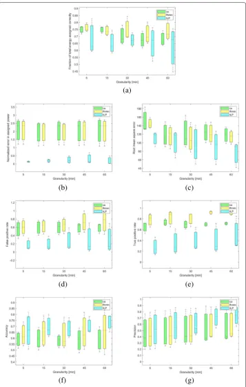
In Fig. 1 we report seven different performance indicators obtained by validating the three algorithms on the UK-DALE dataset, for different epoch granularities ranging from 5 to 60 min. As the appliances belonging to the top consuming set differ from build-ing to buildbuild-ing, global metrics are computed by averagbuild-ing the results obtained for the 5 appliances belonging to each building.
It can be noted that the fraction of energy consumption correctly assigned by the ILP algorithm to the top 5 consuming appliances is slightly lower than that assigned by the CO and FHMM algorithms. However, the normalized error achieved by the ILP algorithm is always consistently smaller than the one obtained by the two benchmark algorithms, while the root mean square error achieved by the ILP algorithm is slightly lower than that obtained by CO and FHMM.
The true positive rate of the ILP algorithm remains lower than that of the CO and FHMM algorithms, with FHMM outperforming CO. However, an increase in the true positive rate of the ILP algorithm is observed at coarse granularities (45 and 60 min epochs). The relatively poor performance of the ILP in terms of true positive rate is com-pensated by the very low false positive rate, which is much smaller than that achieved by the benchmark algorithms. This means that, though the ILP algorithm sometimes does not detect some activity periods of the appliances, it almost never fails in detecting off periods, whereas the CO and FHMM algorithms often incorrectly turns on appliances). Overall, the ILP algorithm achieves accuracy and precision ranges comparable to those of the benchmarks, slightly outperforming the benchmarks and showing remarkably smaller interquantile ranges at coarse measurement granularities4.
While there is not a single algorithm that clearly dominates the other ones, the low false positive rate and the relatively good precision and accuracy seems to be features of some importance when feedback is provided to real users, as higher false positives might eventually reduce the user confidence in the algorithm output.
Conclusions
In this paper we have described a novel algorithm for the disaggregation of the overall energy consumption pattern of a household into the single end-uses of each appliance. The proposed algorithm is based on the solution of a quadratic programming problem with mixed integer constraints. In this paper we report the training and the validation of the algorithm on one well known publicly available dataset and its performance has been evaluated for different granularities of the aggregated energy consumption measure-ments, showing that graceful degradation of the disaggregation results is achieved and that still accurate results can be obtained also in the case of data with 15 min resolution,
4Note that the basic version of the algorithm in (Piga et al.2016) achieves lower accuracy than the ILP algorithm with
(a)
(b)
(c)
(d)
(e)
(f)
(g)
Fig. 1Comparison of the performance of the three NIALM algorithms.aFraction of correctly assigned energy
that is a common data temporal resolution available in most commercial smart-metering solutions, where submetering devices are not or cannot be installed.
About this supplement
This article has been published as part ofEnergy InformaticsVolume 2 Supplement 1, 2019: Proceedings of the 8th DACH+ Conference on Energy Informatics. The full contents of the supplement are available online athttps:// energyinformatics.springeropen.com/articles/supplements/volume-2-supplement-1.
Authors’ contributions
All authors have contributed equally to this paper. All authors read and approved the final manuscript.
Funding
This work has been partially supported by the Horizon 2020 project enCOMPASS (Grant N. 723059). Publication of this supplement was funded by Austrian Federal Ministry for Transport, Innovation and Technology.
Availability of data and materials
The source code and references to the datasets can be found athttps://github.com/encompass-project-eu/ disaggregator.
Competing interests
The authors declare that they have no competing interests.
References
Batra N, Kelly J, Parson O, Dutta H, Knottenbelt W, Rogers A, Singh A, Srivastava M (2014) Nilmtk: Anopen source toolkit for non-intrusive load monitoring. In: Proceedings of the 5th International Conference on Future Energy Systems. ACM, Cambridge. pp 265–276
Hart G (1992) Nonintrusive appliance load monitoring. Proc IEEE 80(12):1870–1891
Piga D, Cominola A, Giuliani M, Castelletti A, Rizzoli A. E (2016) Sparse optimization for automated energy enduse disaggregation. IEEE Trans Control Syst Technol 24(3):1044–1051
Zeifman M, Roth K (2011) Nonintrusive appliance load monitoring: Review and outlook. IEEE Trans Consum Electron 57(1):76–84
Zoha A, Gluhak A, Imran M, Rajasegarar S (2012) Non-intrusive load monitoring approaches for disaggregated energy sensing: A survey. Sensors 12(12):16838-16866
Publisher’s Note
Springer Nature remains neutral with regard to jurisdictional claims in published maps and institutional affiliations.
Submit your manuscript to a
journal and benefi t from:
7Convenient online submission
7Rigorous peer review
7Immediate publication on acceptance
7Open access: articles freely available online
7High visibility within the fi eld
7Retaining the copyright to your article