R E S E A R C H
Open Access
Increasing sensor reliability through
confidence attribution
Roberto M. Scheffel
*and Antônio A. Fröhlich
This work is based on an earlier workWS N Data Confidence Attribution Using Predictorspublished in the Proceedings of
the 8thLatin-American Symposium on Dependable Computing (LADC) in 2018.
Abstract
The reliability of wireless sensor networks (WSN) is getting increasing importance as this kind of networks are becoming the communication base for many cyber-physical systems (CPS). Such systems rely on sensor data correctness to make decisions; therefore, faulty data can lead such systems to take wrong actions. Errors can be originated by sensor’s hardware failures or software bugs and also from the intentional interference of intruders. The gateways that connect such WSN to the Internet are natural intruders’ targets as they usually run conventional operating systems and communication protocols. This work proposes a confidence attribution scheme, based on lightweight predictors running on the sensors. The solution also proposes a parameterizable formula, in order to stamp every value sent by a sensor with aconfidence level, calculated upon the values of a subset of correlated sensors. This work also presents an algorithm that can identify a defective sensor into its subset. The use of predictors and confidence attribution are proposed as the basis of a mechanism that increases the WSN resilience against sensor failure or bad data injection by intruders. Several simulations were performed to evaluate the detection efficiency against different types of sensor errors. This work also analyses mechanisms to deal with concept drifts in the WSN lifetime.
Keywords: Wireless sensors networks, Confidence attribution, Fault detection
Introduction
The advances in the embedded systems technology brought the use of WSN to a variety of application fields. Smart buildings, environmental monitoring, industrial plants, and many other environments can be sensed and controlled by cheap devices, equipped with sensors and actuators, communicating on a wireless network. As these networks are getting integrated into the Internet of Things (IoT), it is essential that they operate in a reliable and trustful manner. Many times, these networks are deployed in harsh environments and are susceptible to interference in sensing and communication. Therefore, fault toler-ance mechanisms are essential to ensure correct readings and actuations by the WSN elements. Faults in a WSN can range from incorrect sensor readings, communication
*Correspondence:[email protected]
Software/Hardware Integration Lab (LISHA), Computer Science Department, Federal University of Santa Catarina (UFSC), PO Box 476, Campus Trindade, 88040-900 Florianópolis, SC, Brazil
failure caused by environmental or intentional interfer-ence, to nodes and gateways intrusion by attackers to forge sensor readings or send incorrect commands to actuators. Although the use of redundant devices increases the fault tolerance in WSNs, consensus or voting algorithms are needed to identify a faulty sensor from the good ones. Several solutions were proposed in the literature, and the majority uses special messages to decide if there was an error and to determine the source. This leads to overhead in terms of latency, bandwidth, and energy consumption in the WSN. Hierarchical or centralized architectures try to minimize this overhead but are subject to errors if the data received is altered by malicious or defective nodes while it is transmitted.
The solution proposed in this work provides self-diagnosis capabilities to the sensor nodes, based on data gathered from correlated neighbors, incurring little com-munication overhead. To accomplish this, an artificial neural network model is built offline for every type of
sensors nodes in an interest area, based on the readings from other correlated sensors in the same area. This model is transferred to the sensor. At runtime, each sen-sor listens to the data transmitted by other nodes in the interest area and uses the model to predict its own value. Comparing the sensed value with the predicted one, each node is able to calculate its confidence or probability of correctness. When the confidence reaches a lower bound, a second step is performed, trying to determine if the node is really faulty or if the discrepancy between the sensed and the predicted value was caused by a faulty neighbor. Every node transmits its sensed value, the predicted value, and the confidence level, to provide information about its current state to the application and to the other corre-lated nodes. This work is an extension of [1], describing the whole architecture, but only the confidence attribu-tion scheme is completely implemented and evaluated. It extends the study of the parameters’ effect on the algorithm’s efficiency and makes a verification of how the proposed solution handles different types of errors.
The actual main approaches used to identify faulty nodes in wireless sensor networks are presented in “Related work” section. “Confidence attribution using predictors” section describes the proposed solution, the architecture, and the algorithm used to assign confidence to values read in each node. Afterward, in “Case study” section, the solution is evaluated through a set of exper-iments on data of a set of real sensors data, and in “Comparison with the hybrid fault detection method” section, a comparison with another algorithm is made using a public dataset. “Concept drift detection” section discusses aspects of concept drift detection on the sce-nario of correlated sensors models, and “Data confidence as trust mechanism” section describes how the proposed mechanism can be employed to enhance the reliability of data received from the WSN at the gateways or at the servers. Finally, the conclusions and future work are presented in “Conclusions” section.
Related work
A standard solution to increase the dependability of a wireless sensors network is the deployment of redun-dant sensors to compare readings. It demands a dense deployment of sensors to allow the identification of the faulty sensor among the correct ones. To avoid the dense deployment of sensors, several alternative methods were proposed to verify the correctness of the sensors’ data. These methods can becentralized, running on the server, distributed, running on the sensor nodes, orhierarchical, when some particular nodes—like the cluster heads— collect data from a set of nodes and run the diagnosis algorithms [2].
The errors in the sensor’s readings were classified by [3] and [4] in four main types.Outliersare isolated readings
that differ significantly from normal readings expected by the models. The spike or peak errors are readings that deviate too much from the normal values for a cer-tain period of time. They are composed of at least a few data samples, and not an isolated reading as an outlier. The third type is the“stuck-at” error, when the readings present a zero (or very little) variation for a period greater than expected. The amount of time in which the reading has to be “flat” to be considered a “stuck-at” must be deter-mined for each type of sensor. Finally, the high noiseor varianceis the occurrence of unusually high variance in the sensor’s readings, in such a way that it differentiates it from the usual noise which appears in many sensor types. Recurrent neural networks (RNN) were used by [5] to predict sensors values, based on previous readings of the sensor and its neighbors. The assumption is that sensors are of the same type, and that difference between the val-ues read by neighbor nodes is bounded by a constant value
. After building and training the RNN, the difference between the sensed value and the predicted value is com-pared to a thresholdη. If the difference is greater thanη, the node is considered faulty.
Time series analysis combined with a voting schema is presented by [6], assuming that all nodes sense the same phenomenon, neighbors can communicate directly, and faults occurs interrelatedly. The autoregressive-moving-average —ARMA(p,q)— model is applied, with pautoregressive terms andqmoving-average terms. The calculation of the regression formula’s parameters is done on readings that are known to be correct, before the sen-sors’ deployment. In the voting phase, the readings of the neighbors are collected. Then, the median of these read-ings is calculated and compared with the actual reading of the sensor. If the difference is greater than a thresholdτ, the read value is considered faulty. Faulty values are not included in the node’s history, to not disturb the moving average used in classification.
Landγ. A modified three-sigma edit test is proposed by [8, 9], using the ratio between the current value, the median and the normalized median absolute deviation of the last n readings. If this ratio is greater than 3, it considers the reading an outlier and the sensor as faulty.
The distributed Bayesian algorithm (DBA) is presented by [10]. Sensors of the same type calculate the probability of being faulty in three steps. First, the nodes periodically exchange their values and probabilities to the other nodes in radio range R. Sensors are in the same state (faulty ornot faulty) if the difference between their readings is smaller than a specified threshold rt. The Bayesian for-mula is used to calculate the fault probability of each node. In the second step, adjustments are made to avoid that a good node surrounded by faulty nodes becomes faulty (and vice versa). In the third step, nodes with a fault prob-ability higher than a given thresholdτwill send a warning message to the sink.
A distributed fault detection based on hidden Markov model is presented in [11]. Each node uses the difference between its value and the values of the neighbors, deter-mining its state aspossibly normal orpossibly faulty. In the sequence, the probability of the node to change its state fromgoodtofaulty(or vice versa) is calculated using a transition matrix built from the results obtained in the first step. The algorithm assumes a WSN composed by a dense deployment of sensors of the same type, to directly compare readings.
A fault-tolerant algorithm for event detection in WSNs is proposed in [12], called spatiotemporal correlation based fault-tolerant event detection (STFTED). The pro-posed scheme uses a location-based weighted voting scheme (LWVS). It explores the spatiotemporal correla-tion between sensor nodes, assuming a dense deployment of sensors of the same type, to detect events. It also assumes a mean valuemnrepresenting a normal reading (or absence of event) and a mean valueme representing the presence of an event. At the node level, the readings of the neighbors are weighted based on their distance. Closer nodes have a higher influence in the estimation function, and vice versa. In this step (LWVS), an estimatorRn for the state nodenis calculated, which can be inaccurate. So, the second step (STFTED) uses the Bayesian formula to calculate the probability of a node to be faulty, based on the estimation of other nodes in the samefault range. If the majority of nodes have a high likelihood of normal readings, abnormal readings are considered faulty, and the contrary is also true.
The authors of [13] proposed an algorithm named fault detection scheme (FDS), also based on a local step, car-ried out on sensor nodes and a second decision step that runs on the cluster head nodes. On the local step, each node calculates the probability of nodeibe faulty (joint probability orPJi), using a Bayesian network that uses the
energy level and the sensed data of nodei(ELiandSDi). If the probability of being faulty exceeds a thresholdδ, the node classifies itself aspossibly faulty(PF). Otherwise, it classifies itself aspossibly normal(PN). Each node sends PJiand its decision to the cluster head (CH), which exe-cutes the second step of the scheme. The CH maintains a table called probability join table (PJT) with thePJ of every node from the cluster. For each node i, the PJT contains the previous and the actualPJi. When the node decision isPFand the difference betweenPJit+1, andPJit is greater than a thresholdγ2, then the node is
consid-ered faulty. Otherwise, it is considconsid-ered a false alarm. Based on FDS, the authors proposed a distributed fault-tolerant algorithm (DFTA) in [14], where they describe a scheme to make the elimination and the recovery of faulty nodes.
A method based on logistic regression is proposed in [15], with the model construction (called Learning Step) executed on the sink, processing data from all sensors. After training the model, it is sent to the nodes, where it is executed. The value predicted by the model is com-pared to the one read by the sensor. If the difference is greater than a threshold, the node is classified as faulty; otherwise, it is classified as normal. No method to deter-mine the threshold value is proposed, and the authors decide it “based mainly on experience and intuition.”
In [16], a distributed fault detection for WSNs in smart grids is presented, based on credibility and cooperation among sensors. Each sensor evaluates its status as suspi-cious or not, based on the mean and the variance of a win-dow containing the lastk-sensed values. A healthy sensor keeps the variance bounded. When a sensor detects itself as suspicious, a diagnostic request is sent to the neigh-bors, and the diagnostic response messages are used to determine the node’s state. After receiving the response of sensors in an area determined by a radiusR, the node can update its probability of being healthy or faulty.
Neural networks are used in [17] to detect and classify different faults in a WSN of homogeneous sensors. The work assumes that the sensors are uniformly distributed and with a set of anchor nodes (cluster heads) that have broad radio range and are fault free. A genetic algorithm combined with gradient descent is used to train the neural networks. These neural networks classify the state of the nodes. After node classification as secure or faulty, the last ones are disconnected from routing paths.
classifier uses the readings of a sensor and from the neigh-bor nodes as input. All classifiers run on the gateway, in a centralized way. The outputs of the classifiers are then joined in a single decision and an estimated value, using weighted majority voting.
Most of the presented solutions use a dense deployment of sensors of the same type, comparing values that should be equal or very similar. The main difference between them is the prediction model, and some of them use extra packet exchange in voting rounds [13] or for value testing [7]. Although it is a possible and realistic WSN configuration, these models are not applicable when sens-ing a variety of values (e.g., environmental monitorsens-ing). Replication is essential to ensure reliability, but the pre-sented solutions demand dense deployment ofeachtype of sensors. This raises costs and causes communica-tion interference and network overload. The proposed solutions also rely on determining models and parame-tersbeforethe WSN deployment, not considering future environmental changes. Extra packet transmissions in diagnostic phases as in [16], or exchanging test results like in [7], causes communication overhead and introduce delays every time a node’s failure occurs.
The fault detection scheme proposed in [13] and [14] uses a hybrid algorithm, with a step carried out on the node, and another performed on the cluster head, which has higher processing and memory capabilities. In oppo-sition to [17], the proposal of this paper is not to auto-matically disconnect faulty nodes, but allow each node to determine its confidence on the sensed value. This can be used to identify a faulty node, as well as to detect data corruption by intermediate nodes. Nevertheless, the application can also cancel the interest on faulty nodes, making them stop sensing until they can get maintenance. The objective of the local confidence determination of the sensor read value proposed in this work has as objective to avoid extra messages exchange between the neighbor nodes to verify faults and identify their origin. It also provides a local algorithm that can attest the data reli-ability to make local decisions safer. Finally, it provides a security increment, as an intruder cannot forge data with-out getting the exact model and input parameters involved in the confidence attribution process.
Confidence attribution using predictors
Decentralized fault detection approaches try to minimize the message and time overhead inherent to a centralized approach but have to deal with limited input sets and less computational power to perform its work. Models used to perform fault detection at the sensor level have to take into account the resource constraints. As radio communication is the most power-consuming resource on a WSN and packet collision is a problem in WSNs with a large number of sensors, or with high sampling
rates, diagnosis messages for fault detection should be avoided.
The fault detection techniques can be applied at differ-ent levels and classified in several ways. When considering the parties involved in the process, they can be classi-fied into three different classes. In aself-diagnosismethod, the node itself can identify faults on its components. In a group detectionmode, each node monitors the behavior of other nodes to detect errors. When using ahierarchical detection, the detection is shifted to more powerful nodes, such as cluster heads or the gateway. In the WSN perspec-tive, the ideal fault detection method would be distributed and use a self-diagnosis approach. A group detection approach can also be used, but in a “speculative mode”, without the use of specific diagnosis or control messages.
The assumption made in this work is that the network is composed of different types of sensors, monitoring several aspects of the same phenomenon or different intercon-nected phenomena. So, it can be assumed that each node produces data correlated with the data produced by some other nodes. The network has to be designed in a way that in different interest areas is a set of sensors that produce correlated values. The size of this set is not fixed and can vary concerning the correlation between the sensed phys-ical quantities. Another assumption is that every node can read the data transmitted by the other nodes. If the communication is ciphered, some global or group key schema has to be used. Messages can be encrypted with a group key, allowing the data reading by other authenti-cated nodes. For authenticity, the messages can be signed with the node’s private key, avoiding the message content from being altered by other nodes.
The proposed scheme aims to provide nodes with self-diagnosis capabilities, based on data gathered from cor-related neighbors, with no communication overhead. For every node type in an interest area, a predictor model is built offline, based on past readings from the different types of sensors in this area. This work uses artificial neu-ral networks, but any other predictor could be used. The only requirement is that the model has to be easily trans-mitted over the network and not demand much memory or processing capabilities. This model (or the new param-eters, when updating a model) is then transmitted to the sensor, where it is stored and executed.
and the confidence level, to provide information about its current state to the application and the other nodes. There is no extra packet transmission, only an increment in the size of the transmitted packet. Assuming a 64-bit value as a sensor reading, the increase is 9 bytes: the predicted value plus one byte for the confidence (a value between 0 and 100). If more confidence levels are needed, more bytes can be added to the packet. It is a design decision whether more granularity in the confidence levels is worth the increment on the network packet size.
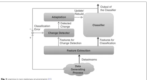
In several monitored environments, the measured val-ues can change in range, and their correlations may vary over time, characterizing many WSNs asnon-stationary environments. The authors of [20] present a process flow for anomaly detection under such conditions, composed of five sub-processes, enumerated below:
1. Change detection: achieved through data monitoring to detect changes in the data distribution. If a significant change occurs, then a model update must be performed.
2. Training set formation: the data vector for model construction and training is formed using sliding windows techniques, discardingn oldest samples and addingn new samples to the training set.
3. Model selection: the optimal parameter set is determined for the new training dataset.
4. Model construction: with the parameters determined in the previous step, a new model is constructed. It can be done inbatch mode, where themodel(t−1)is discarded and the newmodel(t)is built from scratch, or in anincremental mode, wheremodel(t−1)and n new data vectors are used to buildmodel(t). 5. Anomaly detection: the newmodel(t)is used as the
new anomaly detector for fresh dataXt+1,Xt+2,. . ..
The learning framework proposed by [21] shown in Fig. 1 applies to such environments. When a change is detected, the model is updated and sent to the classi-fier. When applying this framework to WSNs, thefeature extraction,change detector, andadaptationprocesses can run on a dedicated server or the Cloud, in a centralized approach. Once the model is built or updated, it can be transmitted to the WSN nodes and used to assign confi-dence to their readings. It can be the sensor node itself or intermediate nodes, in a hierarchical architecture.
The first step is the model building for a specific sensor, based on the historical data from the sensors of an inter-est region. This implies that anewWSN will not have a reliable predictor on its first deployment. After some time running, the data collected by the sensors can be used to train a primary model for each sensor and deliver it to the sensors. Afterwards, an update can be performed every time the adaptation process achieves a more accurate model.
The feature selection process searches the smallest input set for a predictor that produces the best results concerning accuracy and model size. This process can be resource and time-consuming, as many combinations of the inputs have to be evaluated. For large input datasets, or when the correlation between the variables is unknown, automatic attribute selection techniques can be employed. There are several algorithms for this, with different approaches. These algorithms can be grouped into three classes [22]. Filter methods use statistical measures to assign a score to each feature and create a ranking. The lower ranked features are removed from the dataset. The methods are often univariate and consider each feature independently, or about the dependent variable. Some examples of some filter methods include the chi-squared test, information gain, and correlation coefficient scores. Wrapper methodsconsider the selection of the feature set as a search problem. Different combinations are prepared, evaluated, and compared to each other. A predictive model is used to evaluate a combination of features and assign a score based on model accuracy. The search pro-cess may be methodical as a best-first search, stochastic as a random hill-climbing algorithm, or heuristic-based like forward and backward passes to add and remove features. An example of a wrapper method is the recursive feature
elimination algorithm. Embedded methods learn which
features increase the model accuracy while it is created. The most common type of embedded feature selection methods are the regularization methods. Regularization methods—also called penalization methods—introduce additional constraints into the optimization of a predic-tive algorithm (such as a regression algorithm) that bias the model toward lower complexity (fewer coefficients). Examples of regularization algorithms are the LASSO, elastic net, and ridge regression.
Fig. 1Learning in non-stationary environments [21]
model building and training are performed offline, using historical data from a database.
After identifying the set of sensors that are more corre-lated to the target sensor, a model for each node was built automatically. In the first experiments, multilayer percep-trons were used. The number of layers and neurons in
each layer can be determined by heuristics and by rules. The input layer has one neuron for each input value. An extra input can be used for backpropagation or bias. The output layer has one neuron, corresponding to the predicted value. Rules like the proposed by [25] can deter-mine the number of neurons in the hidden layer. Pruning
methods [26] can determine the optimal number of neu-rons in the hidden layer. Once built and trained, the models are transmitted to the respective nodes.
When the predictor is received, sensors can start to determine the correctness of their readings. The confi-dence level C of a node is a function that evaluates the difference between the predicted valuevˆ and the sensed valuev, soC=f(v,vˆ), withf as described in Eq.1. In this work, themean absolute error(see Eq.2) obtained in the training process is used to calculate the result of the func-tion. Comparing it to the root square mean error (RSME), the authors of [27] state that MAE is a natural measure of average error and is unambiguous, being widely used for model-performance evaluation.
f(v,vˆ)=
1, if |v− ˆv| ≤β×MAE
1− |v−ˆvα|−×MAEβ×MAE, otherwise (1)
MAE= 1
n n
i=1
|vi− ˆvi| (2)
The constantsαandβadjust the sensitivity of the func-tion1. The value ofβdefines the tolerance margin (rela-tive to MAE) that considers a value correct with 100% con-fidence. If the model has good accuracy, a small value ofβ can be used to detect small variations in the readings. Oth-erwise, if the monitored value presents high variability, this constant has to get a larger value in order to accom-modate the variations. The value ofαdefines the “velocity” that the confidence decreases as the difference between the predicted and the monitored value increases. The smallerα, the faster the confidence decreases. If the pre-dicted and monitored values are too distant from each other, the function may result negative, in which case the confidence assumes 0 (zero).
The prediction models may show circular references (the model to predict variableS1depends on variableS2,
and the model to predictS2depends onS1), since the
cor-relation is reflexive. The monitoring applications of WSN perform periodic sampling of the sensor values. So, we assume that it is possible to determine a periodP, in which at last one reading of each sensor type is transmitted to the application. The majority of WSN communication proto-cols do not guarantee the order between messages while they are retransmitted by the intermediate nodes. Also, the exact instant when a message arrives on a node is not determined only by the instant it is produced. It is also highly influenced by communication delays and network load. The protocols only guarantee that data is delivered at each periodP, without ordering guarantees. So, it is only possible to assume that the data from the previous period is available. Therefore, models are trained using data from the last period to predict the values of the actual period. Each node will passively listen to the data sent by other
nodes, collecting the inputs for its predictor. Data pro-duced by the nearest sensor of the input types of its model will be buffered. This data will then be used as input val-ues of the model for the local node, in the next periodt+1 (Eq.3).
ˆ
vti+1=fvt1,vt2,vt3,. . .,vtn, for allninputs (3) As the environment changes, thechange detector pro-cess presented in Fig.1has to detect the changes and trig-ger the adaptation process. Change detection methods can be grouped into four main families [21]:
• Hypothesis test uses statistical techniques to verify the classification error of a fixed-length set of readings. The variation of the classification error is compared to the error of the training dataset. • Change-point methods also uses a fixed-length data
sequence, analyzing all partitions of the data sequence to identify the instant when the data changes its statistical behavior, called change-point. The main drawback of this method is the high computational complexity.
• Sequential hypothesis test instead of analyzing a fixed-length window of data, this method inspects each incoming sample, until they have enough evidence that a change has occurred or not. • Change detection tests are specifically designed to
analyze the statistical behavior of data streams sequentially. Most of them operate by comparing the prediction of absolute error or its variance to a specified threshold. The threshold is hard to determine at design time. Some adaptive algorithms were proposed, using cumulative errors.
The authors also propose the use of hybrid change detec-tion. A change detection test can be used in a first layer, followed by a validation layer that uses a change-point method.
Model update, performed after a change is detected, consists in retraining the model with new data. The main approaches arewindowing,weighting, and random sam-pling. At this step, one of the main questions is if the model has to forget the oldest rules and reinforce the new ones, or if the learning has to be cumulative. In the for-mer case, the model is entirely retrained using new data. This implies retraining the model every time a change is detected but can lead to smaller models. The latter case, incremental learning can keep past knowledge, but models tend to be larger, demanding more memory and processing.
gather enough data to build and train models for the dif-ferent sensors. Models are then built for each type of sensor in the same region and can be sent to them in agroup communication. The application can control the model transmission frequency to avoid network flooding. Model updates are expected only when the correlation between the sensed values changed. In a training phase, some overhead will happen when some models have to be updated. After some time—that depends on the envi-ronment dynamics—it is expected to occur very rarely. The compressed size of the model (around 3 KB) makes it feasible to be transmitted over the WSN. The proposed solution does not fit well to environments where the cor-relations are changing continuously at a high rate. The use of cumulative learning, although producing larger mod-els, was chosen in the first experiments as it is expected that environments with cyclic changes willstabilizeover time in the learning process, demanding much less (or even none) updates after running for a period. The dif-ferent approaches for drift detection and model retraining are still under evaluation and a discussion about it is made in “Concept drift detection” section.
Fault Identification and the interference problem
If each node sends only the value of the sensor and its confidence, it would be hard for other nodes to make a reasonable statement about its confidence on the sensed value. It happens because a wrong input in the model causes distortions in the output, leading to an erroneous confidence attribution. For this reason, fault detection algorithms tend to use voting or joint probability tables to identify the fault source. In the scheme proposed in this work, every node sends three values: the sensed valuev, the predicted valuevˆ, and the confidence levelC. Knowing these three values from the correlated neighbors, every node is able to autonomously verify the correctness of its readings, without extra messages. On receiving an input valuevwith low confidence, the local predictor will use the predicted input valuevˆto calculate its prediction and confidence for local v. Doing so, the failure of a sen-sor will take longer to affect other sensen-sors’ confidence by interfering in their prediction models. It also enables the identification of the faulty node, as it will show lower confidence, unlike the other (well functioning) sensors. At each node, the algorithm that performs the process of confidence attribution shown in Fig.2is described in Algorithm 1.
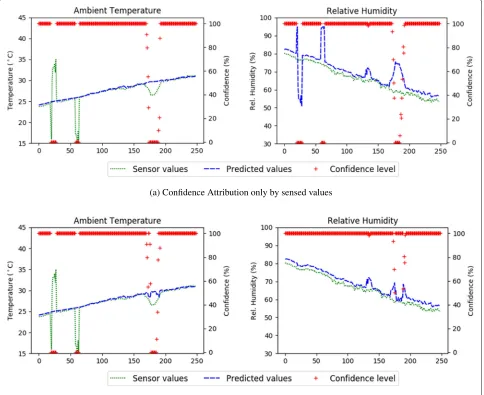
Applying only the Eq.1to the sensed values of the cor-related sensors will cause an error spreading as illustrated in Fig.3a, leading to aninterference problem. As the read-ing faults occur in the first sensor (ambient temperature), the predicted values of the second sensor (relative humid-ity) change proportionally, but in the opposite direction, once they show an inverse correlation. If no information
Algorithm 1Confidence Attribution Routine
1: procedure Confidence_Attribution
2: // Calculates the predicted value based on sensed values 3: voˆ ←model(values)
4: diff← |y− ˆvo| 5: ifdiff≤(β∗MAE)then 6: confo←100 7: else
8: confo←(|y− ˆvo| −β×MAE)/(α×MAE)×100 9: ifconfo<0then
10: confo←0 11: end if 12: end if
13: // Changes low confidence readings to the predicted values 14: for eachci∈confidencesdo
15: if(ci< γ )then
16: values[i]←predictions[i] 17: end if
18: end for
19: ˆvp←model(values) 20: diff← |y− ˆvp| 21: ifdiff≤(β∗MAE)then 22: confp←100 23: else
24: confp←(|y− ˆvp| −β×MAE)/(α×MAE)×100 25: ifconfp<0then
26: confp←0 27: end if 28: end if
29: if(confo>confp)then 30: return(v,ˆvo,confo) 31: else
32: return(v,ˆvp,confp) 33: end if
34: end procedure
Fig. 3Fault isolation by Algorithm 1.aThe predictions of Relative Humidity are distorted by ambient temperature.bThe algorithm isolates the distortion when confidence goes bellowγ
In the next section, a case study is presented, illus-trating the whole process and making an analysis of the impact of different values of the algorithm’s parameters (α, β, and γ). Despite using artificial neural networks and the previously presented confidence formula (1), the proposed solution can be changed in several ways. The central point of the architecture is the use of apredictor, a confidence attribution formula, and the use of the output of other sensors (read value, predicted value, and confi-dence) to determine origin of a fault. Any component can be replaced. Another type of predictor or a specialized confidence formula can be employed, without significant impact on the proposed schema.
The main reason use of a predictor and a confidence attribution formula instead of a classifier is because the objective is to be able to detect the different levels of
variation on the read values, not just classify the values ascorrect or incorrect (and some intermediary classes). The confidence level can be adjusted to a large number of levels, only by adjusting the number of bytes used to represent it, determined by the application’s needs, by the sensors’ processing capabilities or by the number of bytes available in the network packets.
Case study
power plant and subsequently cleaned and validated by the engineers that commissioned the plant. Segments corresponding to 5% of each time series were used to perform feature selection with the SelectKBest selector from the scikit-learn framework.
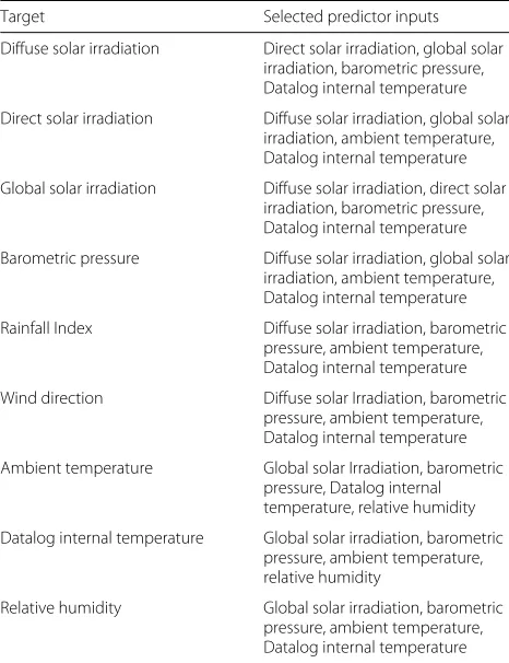
For each variable, the six other variables with the high-est correlation were selected to be used as the predictor’s input. The variables and the selected features are shown in Table 1. The hour and minute of each datapoint’s timestamp are recurring features that are relevant to all variables. The month of the year, which would have been a good indicator of the seasonality of solar energy gener-ation, was not detected as a feature because the training data covered less than 1 month. This will intentionally make the model susceptible to concept drifting, and it will be shown and discussed in “Concept drift detection” section.
After the feature selection, an artificial neural network (ANN) was built for every sensor, using the multilayer perceptron architecture. All ANNs have the same struc-ture, with six neurons in the input layer (one for each feature), five neurons in the hidden layer, and one neuron in the output layer. The Keras API [29] and the Theano library [28] were used to build, train, and evaluate the ANNs. The small size of the model makes it suitable to be transmitted to the sensor nodes and executed locally
Table 1Feature selection result
Target Selected predictor inputs
Diffuse solar irradiation Direct solar irradiation, global solar irradiation, barometric pressure, Datalog internal temperature
Direct solar irradiation Diffuse solar irradiation, global solar irradiation, ambient temperature, Datalog internal temperature
Global solar irradiation Diffuse solar irradiation, direct solar irradiation, barometric pressure, Datalog internal temperature
Barometric pressure Diffuse solar irradiation, global solar irradiation, ambient temperature, Datalog internal temperature
Rainfall Index Diffuse solar irradiation, barometric pressure, ambient temperature, Datalog internal temperature
Wind direction Diffuse solar Irradiation, barometric pressure, ambient temperature, Datalog internal temperature
Ambient temperature Global solar Irradiation, barometric pressure, Datalog internal temperature, relative humidity
Datalog internal temperature Global solar irradiation, barometric pressure, ambient temperature, relative humidity
Relative humidity Global solar irradiation, barometric pressure, ambient temperature, Datalog internal temperature
to make the predictions. After the ANNs were built, the MAE was calculated over the training dataset for each variable, as shown in Table2. As an example, the MAE value for the ambient temperature makes a value ofvbe considered having 100% confidence if it lies in the range [vˆ−0.41697,ˆv+0.41697], wherevˆis the predicted value, whenβ= 1.0. This interval can be shrunk or stretched by modifying the value ofβ.
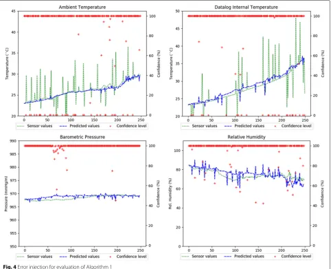
Once the model building phase was finished, several simulations were carried out to verify the accuracy of the proposed confidence attribution scheme. Five differ-ent data chunks were extracted from the original dataset, each one with 1440 samples (1-day sampling). The eval-uation was done in two steps. First, to evaluate the mod-els efficiency in identifying and isolating errors in one sequence (its origin), several errors of theoutliertype [4] were injected at random points in the data in the ambi-ent temperature and the Datalog internal temperature sequences. One hundred forty-four errors were injected in each sequence, independently, and 144 errors were injected simultaneously on both sequences. The objective of injecting simultaneous errors in both sequences was to verify if the substitution of read value by the predicted one in a sequence would lead Algorithm 1 to mask the error on the other sequence. Algorithm 1 was executed on the data chunks, measuring the detection and false positives rates. The variation of the three algorithm parameters—-namely
β,α, andγ—allowed to verify their influence on the algo-rithm efficiency. In the next set of experiments, the other three types of error defined by [4]—peaks,“stuck-at,”and noise—were injected in the data sequences, to verify the algorithm sensitiveness to each type of error. The objec-tive was to verify if errors are correctly detected when the values deviate significantly from the normal ones. No error classification is expected in this work. So, if different types of error appear, causing significant deviation on the monitored values, the algorithm only assigns a lower con-fidence to the variable, no matter what kind of error has occurred.
Table 2MAEs calculated for predictors
Sensor Model’s MAE
Diffuse solar irradiation 2.5799
Direct solar irradiation 15.8076
Global solar irradiation 16.2823
Barometric pressure 0.7605
Rainfall Index 0.0017
Wind direction 28.9098
Ambient temperature 0.41697
Datalog internal temperature 0.7318
Figure4 shows the effects of injecting outliers in the
sequences of the ambient temperature and the
Data-log internal temperaturevalues. The peaks in the values (green dotted lines) on the two top graphs show the points where the errors were injected, at random instants. The peaks in the predicted values (blue dashed lines) show the effects of the injected errors in the predictor’s output of the related variables. When the incorrect input leads to confidence lower than the threshold defined by γ (40% in this experiment), the algorithm makes the substitution by the input’s predicted value, trying to get the predicted value closer to the range of correct values if its value is correct. So, it is normal that small peaks appear on the predicted values.
Algorithm parameter evaluation
To evaluate how the algorithm parameters influence on the results, several errors ofoutlier type were randomly injected in each data chunk. The amplitfude of the error
was also randomly defined. So, it is expected that not everyerror is detected with confidence bellowγ, as some generated values can fall inside the range of acceptable values. The ambient temperature and the Datalog internal temperature sequences were chosen to have their values changed, as they are input for all other predictors, and also show high interdependence. The errors were injected as described previously. The process was repeated ten times with each data chunk, and the mean values of the detection and false positive rates were calculated.
Theerror detection rate(EDR) is the percentage of the injected errors that are correctly identified by the pro-posed algorithm. Afalse positiveoccurs when a node with no error injection presents a confidence level below theγ parameter (Algorithm 1, line 15), at the next period where an error was injected in another sequence. As explained in formula3, each read value is used as input of the pre-dictors in the next time period. This implies that low con-fidence on this variable results from a wrong prediction
caused by the injected error. This is unexpected and the algorithm tries to eliminate, or at least to minimize, its impact. As some errors may occur in the sample data—as it is data from real sensors—the confidence of all variables before the error injection was calculated and stored. For each low confidence found after the error injection, it was compared with the recorded value. So, false positives were counted only whennewerrors were detected. The false positive rate(FPR) is calculated based on the num-ber of injected errors, making it possible compare the results of experiments made with different sizes if input set and different numbers of injected errors. The formu-las areEDR=(detected_errors×100)/injected_errorsand FPR=(false_positives×100)/injected_errors.
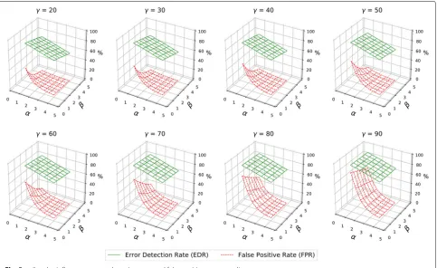
The experiments results are shown on Fig.5, with the minimum confidence (γ) varying from 20 to 90 in inter-vals of 10, and α and β varying from 1.0 to 4.0 in a step of 0.5, making a total of 392 evaluated combinations. As explained before, a small value of β means that the current reading can show only a little discrepancy from the predicted one to be considered 100% correct. The opposite is true for larger values of β. Theα parameter determines the width of a range of values where the con-fidence decreases from 100 to 0%. The wider the range, the slower the confidence decreases. So, small values of
αmake the algorithm drop confidence very fast, and vice versa. Finally, theγ parameter defines the confidence level
below which the algorithm tries to replace the read values by the predicted ones, searching for a possible error. The lower the value of this parameter is, the more“lenient”the algorithm is with the investigation of possible errors.
The objective is to maximize the number of detected errors and, at the same time, to minimize the number of false positives injected. So, the best combination of parameters will be the one that gets the biggest differ-ence between these two results. Figure5shows the EDR and FPR values obtained for every combination of the three parameters. The highest EDR were obtained using the most restrictive combination of parameters (β = 1.0,
α = 1.0, andγ = 90), detecting 94.2% of the injected errors. But this combination also shows the highest FPR, as high as 79.5% of the injected errors. This is expected because any reading that deviates 1.1 times the MAE from the model will be considered an error and tested against the predicted value. The FPR decreases for smaller values ofγ. It also decreases as the values ofα andβ increase, with FPR getting close to zero when both parameters are 4.0. The graphs of Fig.5show that average values for all parameters show balanced results.
As the parameters can be individually adjusted for dif-ferent scenarios and application needs, a reasonable start point is setting α and β parameters to a value around 2.5 and γ to 50, and adjusting them until the desired detection and false positive rates were obtained. As just
three numbers must be adjusted, thinking on a distributed environment as a WSN, it is necessary to broadcast a sin-gle message to adjust the algorithm’s parameters on all nodes, or on a subset of nodes of the same type. As the MAE value is expected to be larger for models with highly varying values, the parameters can also be set individu-ally for these type of nodes to get a better tolerance to the variance.
Error type coverage
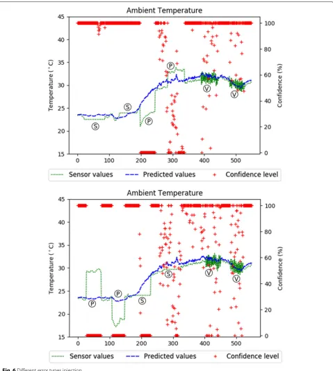
A second set of evaluations was executed in order to iden-tify the algorithm effectiveness on detecting the other three types of errors defined by [4]: peak, stuck-at, and noise. The error injections mechanism was adjusted to generate several sequences of errors in the same data chunks used in the first evaluation. Examples of the injected errors and their correspondent confidence lev-els are illustrated in Fig. 6. On these graphs, each type of errors was injected twice. To better identify each error type, they are marked on the graphs with different letters:
Sforstuck-aterrors,Pforpeakerrors, andVforvariance (ornoise) errors. The parameters used to create the graphs of Fig.6wereα=2.5,β=2.5, andγ =50.
The peak errors are very similar to the outlier errors, used in the first evaluation. So, the confidence level drops as soon as the monitored values deviate enough from the usual (predicted) values. Figure6shows that peak errors are better detected than the stuck-at or variance errors. This happens because peak errors generate values farther from the expected ones. But in some situations, a peak can make the monitored values go into the directions of the predictions, mainly when there is some gap between the real values and the predicted ones. When this hap-pens, the values remain in the range with confidence high enough, and the sequence may not be classified as an error. The second peak of the upper graph in Fig.6 illus-trates this, as the sensors readings get various confidence levels, from 0 to 80, when the peak error is occurring (around sample 300).
The detection of the stuck-aterrors is determined by the data behavior. In the upper graph of Fig. 6, the repeated value is close to the predictions, making the error remain undetected. On the lower graph, however, as the predictions followed the input from the correlated vari-ables, the difference from the constant value increased enough to make the errors be detected. This is reflected by the assignment of different levels of confidence, from 0 to 100.
The proposed mechanism gets low accuracy in identi-fying thevarianceerror when the readings do not exceed the thresholds defined by the α and β parameters. The graphs of Fig.6shows that high variance errors (Vmarks) that keep the values close to the correct ones are not detected. Only when the noise produces values with larger
discrepancies, the confidence of the variable starts to decrease. If the noise makes the monitored values fall too far from the expected ones, the proposed solution will detect them as it does with the outliers. The noise can be an indicator of malfunction or interference, but while it does not causes readings to be too distant from real val-ues, the confidence attribution scheme will not classify this kind of behaviors as an error. This kind of behavior classification is not in the scope of this work. Solutions of variance analysis can be used at the server to indicate noise in a sequence of readings, indicating the need for some maintenance. Noise errors can also be detected if they produce readings outside theβ ×MAE threshold, producing sequences of different, highly varying levels of confidence. Again, this sensitiveness can be adjusted by setting theαandβparameters.
The “stuck-at” is an error type that can show a differ-ent impact on the monitored value confidence,
depend-ing on when it occurs and how long it lasts. When
the monitored variable“freezes” on a value close to the normal values, and the last ones show only small vari-ations, the error is not detected. This is a situation similar to the noise error and is illustrated in the first graph of Fig.6. But when the normal values sequence is ascending or descending—like temperature in the morn-ing or in the late afternoon—then the difference will be detected, and the monitored variable’s confidence will fall in the same rate. This is well illustrated in the first error labeledS on the lower graph of Fig.6. Obviously, if an error makes the readings to be stuck at a distant value, then the algorithm will drop the sensor confidence instantly.
The analysis of the results show that the algorithm can identify errors in sequences that are greater than some thresholdand ignores errors that do not deviate too much from thenormalvalues of the sequence. It does not detect noiseandstuck-aterror when they lay around the normal readings. This types of errors are easily detected by algo-rithms that use statistical analysis on a window of theN last readings. This type of detection and classification is out of the scope of this work. We are interested in identi-fying errors—from failures or intentionally injected by an intruder—that deviates from the correct values and could lead to wrong decisions, e.g., in a cyber-physical system, as well as labeling data with confidence levels to allow check-ing against message corruption when data arrives on the server.
Fig. 6Different error types injection
that can be used to identifynoiseandstuck-aterrors at a second stage, not covered in this work.
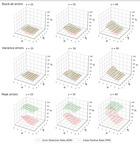
To compare the results obtained with different error types, Fig. 7 shows the results for the combinations of the algorithm parameters α andβ, withγ assuming 20, 50, and 90. Other values of γ were omitted due to lack of space. As already discussed, the EDR and FPR for the
Fig. 7Error detection rates and false positive rates for different types of errors
a more significant statistical impact that one outlier that does the same. If the simulation is adjusted to produce only large deviations when generating peak errors, the results would be practically the same to the obtained with the outlier errors. But this would artificially inflate the EDR and would not follow the original definition of the error type. Thestuck-atandnoiseerrors show much lower EDRs, as the error values were mainly too close to the pre-dicted values. They may cause variation in the confidence assigned to the value while the error occurs, but are not
reported as an error as the confidence remains aboveγ. This is the reason whyγ =90 associated with small val-ues ofαandβresult in higher detection and false positive rates for both type of errors.
Comparison with the hybrid fault detection method
mechanism to one of their datasets available online. The dataset consists of environmental data collected at the Grand Saint Bernard pass between Switzerland and Italy in 2007 [31]. It contains samples of temperature, humid-ity, and solar irradiation collected along 43 days with a temporal resolution of 2 min. The results obtained by applying our proposal to this dataset are compared to the results obtained by the authors [6]. They selected ten sen-sors among the most faulty ones to evaluate the accuracy of fault detection and classification and also applied time series analysis and neighbor voting algorithms to detect four types of failure.
We first aligned the datapoints in time. Two sensors that failed to produce data (their focus was on sensor failure, ours on data confidence) were excluded from the comparison. The resulting dataset contains 20180 data-points. Subsequently, we manually classified discrepant datapoints as faulty. After that, sequences with no faulty data were selected at five different periods of the time series, resulting in a training set of 6800 records. The fea-ture selection procedure was applied next, identifying the relationship among the variables across different sensors.
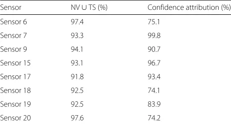
We built the ANNs as described in “Algorithm param-eter evaluation” section and obtained the MAE for every sensor. The models were then evaluated for every sensor with average values:γ = 50,α= 2.5, andβ = 2.5. A node was considered faulty when the confidence reached 0. The compared work counted errors by occurrence in each test intervalT of 30 minutes, no matter how long the error remained. As our proposed algorithm evaluates each dat-apoint individually, a direct comparison of error counts is meaningless. So, the error detection rate (which is called success ratio in their work) will be used for comparison. In their work,neighbour voting (NV)andtime series analysis (TS)were combined to achieve the best results (NV∪TS), which is the basis for the comparison with our mechanism summarized in Table3.
The results show that for some sensors the EDR is sig-nificantly lower than the compared technique. Inspecting the data, it is possible to verify that the causes explained
Table 3Compared algorithm evaluation
Sensor NV∪TS (%) Confidence attribution (%)
Sensor 6 97.4 75.1
Sensor 7 93.3 99.8
Sensor 9 94.1 90.7
Sensor 15 93.1 96.7
Sensor 17 91.8 93.4
Sensor 18 92.5 74.1
Sensor 19 92.5 83.9
Sensor 20 97.6 74.2
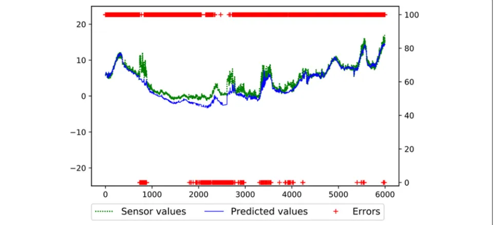
in “Error type coverage” section are present in the eval-uated dataset. Taking as example sensor 18, it is visible that the errors are mainly of thesuck-attype, as shown in Fig.8. For clarity, confidence (red crosses) is only marked at 100 (no error) and 0 (error) to not hide data lines on the graph. The sensor reported−1 for a long time. As the real temperature was around that value for a significant period (around sample 3000), it was not detected as a faulty value because it was in the range of acceptable values. Almost all of the undetected errors are due to the fact that stuck-aterrors are not identified when they are close to the real values. On sensors where mostly peak and outlier errors occur, as for sensor 7, 15, and 17, the error detection rate of our algorithm outperforms the compared solution. Figure9shows the detection of this type of errors on sen-sor 15. On the other hand, in [6] the authors demonstrate that the peak errors (nameddriftby the authors) is the one with lowest detection rates, reaching from 76.9 to 84.6% of accuracy.
Other solutions described on “Related work” section make their evaluations based on proprietary real or sim-ulated WSN, so it was not possible to directly compare results, as data could not be replicated to be used with our algorithm.
Concept drift detection
In this section, we discuss the detection ofconcept drifts. Once sensors may be monitoring dynamic environments, the simulation models are subject to modifications in the correlations between the readings of different sensors in different instants. As described by [32], aconcept is the classification or prediction result of a vector of valuesα. If the result changes over time, i.e.,Pt(χ) =Pu(χ), then aconcept driftoccurs, as the same input setχ produces different results at timest and u, and both are correct. Similarly, [33] defines it as∃χ : Pt0(χ,y) = Pt1(χ,y), meaning that the joint distribution of a set of input vari-ablesχand the target variableymay vary from timet0to
timet1.
Fig. 8Sensor 18 stuck at−1 for a long time
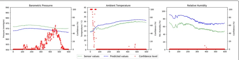
When a concept drift occurs, the predictors built at the server with outdated data will not be able to correctly han-dle that changes. The majority of the models will start to assign lower confidence levels to their data. For example, when the training is made with data obtained in summer days—as in the experiment presented in this work—the model assigns low confidence to relative humidity, ambi-ent temperature, and barometric pressure, as they show correlations slightly different in winter (Fig.10). As shown by the figure, the predicted values are clearly following the
sensor readings but are not close enough to be considered correct.
At the server side—where enough computational power is available—more elaborated algorithms can be used to verify if some sequences are real concept drifts or long lasting errors, like sensors slowly deviating their readings from the correct ones. Models comparing read-ings variations of each sensor and comparing them to the variations in other sensors must be built, mixing sta-tistical analysis and predictions results. Theseensembles
Fig. 10General confidence drop on concept drift
can use some voting mechanism, for example, to decide if a concept drift has occurred. Another solution is use the outputs of all the different detection mechanisms and build and train a classifier to verify if the data streams should be considered errors or concept drifts.
We are evaluating the use of an algorithm that com-bines the outputs of a drift detection method such as the EWMA for the different available values. The idea is to evaluate the behavior of the values and the confidence lev-els of all correlated variables. The algorithm then has to decide if a set of deviations, occurring for a long enough period of time, is an error or a concept drift. We are also investigating other drift detection methods suitable for the given scenario.
Data confidence as trust mechanism
The proposed confidence attribution scheme has shown feasible to be applied to resource-constrained devices, as the model is not expensive in size to transmit and store in the nodes of the WSN. Neither demands high com-putational power to execute. The most power-demanding tasks—feature selection, model building, updating, and training—are performed offline, at powerful servers or on the Cloud.
As the models are built on the server, they can be stored to perform later verification to identify if data was adulter-ated at the origin (the sensor node), when it is retransmit-ted by intermediate nodes, or even by a malicious gateway. Therefore, it increases the overall dependability of the WSN data, as an attack have to occur in a coordinated way on all correlated nodes.
If an intruder forges the values read by a sensorbeforeit enters the confidence attribution schema, it will be identi-fied as faulty and get a low confidence level. The intruder can also try to change a sensor valueafterthe confidence attribution. It can happen on the node, before the values are transmitted, on an relay node or at the gateway. In the last case, to be considered valid by the application and start an incorrect actuation, the false value has to be trans-mitted with high confidence attributed. Before sending
the actuation command, the application can recalculate the confidence of the received value. It only has to apply the algorithm with correlated sensors values as input and check if the result is the same presented by the suspicious node. If a wrong value is presented with a high confidence value, it will not match the confidence calculated by the application. As another side effect, most confidence levels calculated by other nodes that used the false input will not match. The difference will be even worse if the neighbor nodes used the correct values in its calculations and the value is altered afterward, as at the gateway.
To forge plausible incorrect values, an intruder has to get access to all involved models and adjust the predicted values and the confidence levels of all correlated values that will be affected—directly or indirectly—by the forged value. It would be computationally expensive and inviable at the WSN level, due to the number of messages needed to adjust and verify all involved values. It could be possible at the gateway, but other intrusion detection techniques would easily detect the extra processing and retransmis-sions delays while the malicious software tries to calculate the new confidences.
Conclusions
Simulations shown that the proposed solution reaches good accuracy levels in identifying nodes’ data faults and its source. A fault is a value too far from the expected correct value, based on other correlated observed values. Parameters can be adjusted to get the desired algorithm sensitivityor the balance between detection rate and false positives. The solution can also be used to verify the data integrity at the application, comparing models out-puts with the received values at WSN gateways or at the application servers. As any interference on the read values and/or confidence levels can be compared to the output of other model, the proposed mechanism adds an extra authenticity and integrity level to the WSN.
As future work, efforts on the definition of a reli-able change detection methods has to be made, in order to select methods that can address the several aspects involved in correctly identify the occurrence of concept drifts. The results of our preliminary results shown that the statistical and time series analysis on single data streams have to be reinforced by comparing data from different sources. It is expected that suchensemblescan reach better results in this task. On the predictors, the use of Incremental Gaussian Mixture Network (IGMN) [35] will also be evaluated, as that model is resilient to miss-ing inputs. This feature can be useful in networks subject to communication problems, in unreliable environments. The integration of the proposed solution to a communica-tion protocol will also be implemented and evaluated, in order to measure the real impact on energy consumption and the detection of possibly intrusion attempts in WSN and CPS scenarios.
Acknowledgements
The authors would like to thank the support provided by the involved universities.
Authors’ contributions
Both authors contributed equally to this work. Both authors read and approved the final manuscript.
Funding Not applicable.
Availability of supporting data
The dataset used in the experiments is avaliable athttps://lisha.ufsc.br/tiki-list_ file_gallery.php?galleryId=52.
Competing interests
The authors declare that they have no competing interests.
Received: 5 April 2019 Accepted: 4 November 2019
References
1. Scheffel RM, Fröhlich AA (2018) WSN data confidence attribution using predictors. In: 2018 Eighth Latin-American Symposium on Dependable Computing (LADC). IEEE, Piscataway. pp 145–154
2. Khan MZ (2013) Fault management in wireless sensor networks. Comput Sci Telecommun 37(1):3–17
3. Ni K, Ramanathan N, Chehade MNH, Balzano L, Nair S, Zahedi S, Kohler E, Pottie G, Hansen M, Srivastava M (2009) Sensor network data fault types. ACM Trans Sensor Netw (TOSN) 5(3):25
4. Sharma AB, Golubchik L, Govindan R (2010) Sensor faults: detection methods and prevalence in real-world datasets. ACM Trans Sensor Netw (TOSN) 6(3):23
5. Moustapha AI, Selmic RR (2008) Wireless sensor network modeling using modified recurrent neural networks: application to fault detection. IEEE Trans Instrument Measure 57(5):981–988
6. Nguyen TA, Bucur D, Aiello M, Tei K (2013) Applying time series analysis and neighbourhood voting in a decentralised approach for fault detection and classification in WSNs. In: Proceedings of the Fourth Symposium on Information and Communication Technology. ACM, New York. pp 234–241
7. Li W, Bassi F, Dardari D, Kieffer M, Pasolini G (2015) Low-complexity distributed fault detection for wireless sensor networks. In: Communications (ICC), 2015 IEEE International Conference On. IEEE, Piscataway. pp 6712–6718
8. Panda M, Khilar PM (2012) Distributed soft fault detection algorithm in wireless sensor networks using statistical test. In: Parallel Distributed and Grid Computing (PDGC), 2012 2nd IEEE International Conference On. IEEE, Piscataway. pp 195–198
9. Panda M, Khilar PM (2015) Distributed self fault diagnosis algorithm for large scale wireless sensor networks using modified three sigma edit test. Ad Hoc Netw 25:170–184
10. Yuan H, Zhao X, Yu L (2015) A distributed Bayesian algorithm for data fault detection in wireless sensor networks. In: Information Networking (ICOIN), 2015 International Conference On. IEEE, Piscataway. pp 63–68
11. Saihi M, Boussaid B, Zouinkhi A, Abdelkrim N (2015) Distributed fault detection based on hmm for wireless sensor networks. In: Systems and Control (ICSC), 2015 4th International Conference On. IEEE, Piscataway. pp 189–193
12. Liu K, Zhuang Y, Wang Z, Ma J (2015) Spatiotemporal correlation based fault-tolerant event detection in wireless sensor networks. Intl J Distrib Sensor Netw 11(10):643570
13. Titouna C, Aliouat M, Gueroui M (2016) FDS: fault detection scheme for wireless sensor networks. Wirel Person Commun 86(2):549–562 14. Titouna C, Gueroui M, Aliouat M, Ari AAA, Amine A (2017) Distributed
fault-tolerant algorithm for wireless sensor network. Int J Commun Netw Inf Secur 9(2):241
15. Zhang T, Zhao Q, Nakamoto Y (2017) Faulty sensor data detection in wireless sensor networks using logistical regression. In: Distributed Computing Systems Workshops (ICDCSW), 2017 IEEE 37th International Conference On. IEEE, Piscataway. pp 13–18
16. Shao S, Guo S, Qiu X (2017) Distributed fault detection based on credibility and cooperation for WSNs in smart grids. Sensors 17(5):983 17. Swain RR, Khilar PM (2017) Composite fault diagnosis in wireless sensor
networks using neural networks. Wirel Person Commun 95(3):2507–2548 18. Wo´zniak M, Graña M, Corchado E (2014) A survey of multiple classifier
systems as hybrid systems. Inf Fusion 16:3–17
19. Curiac D-I, Volosencu C (2012) Ensemble based sensing anomaly detection in wireless sensor networks. Expert Syst Appl 39(10):9087–9096 20. O’Reilly C, Gluhak A, Imran MA, Rajasegarar S (2014) Anomaly detection in wireless sensor networks in a non-stationary environment. IEEE Commun Surveys Tutor 16(3):1413–1432
21. Ditzler G, Roveri M, Alippi C, Polikar R (2015) Learning in nonstationary environments: a survey. IEEE Comput Intell Mag 10(4):12–25 22. Visalakshi S, Radha V (2014) A literature review of feature selection
techniques and applications: review of feature selection in data mining. In: Computational Intelligence and Computing Research (ICCIC), 2014 IEEE International Conference On. IEEE, Piscataway. pp 1–6
23. Frank E, Hall MA, Witten IH (2017) Data Mining - Practical Machine Learning Tools and Techniques. 4th ed.. Morgan Kaufmann, Cambridge. pp. 553–571
24. Pedregosa F, Varoquaux G, Gramfort A, Michel V, Thirion B, Grisel O, Blondel M, Prettenhofer P, Weiss R, Dubourg V, et al (2011) Scikit-learn: machine learning in python. J Mach Learn Res 12(Oct):2825–2830 25. Trenn S (2008) Multilayer perceptrons: Approximation order and
necessary number of hidden units. IEEE Trans Neural Netw 19(5):836–844 26. Thomas P, Suhner M-C (2015) A new multilayer perceptron pruning
algorithm for classification and regression applications. Neural Process Lett 42(2):437–458
28. Al-Rfou R, Alain G, Almahairi A, Angermueller C, Bahdanau D, Ballas N, Bastien F, Bayer J, Belikov A, Belopolsky A, et al (2016) Theano: a python framework for fast computation of mathematical expressions. arXiv preprint arXiv:1605.02688 472:473
29. Chollet F (2015) Keras: The Python Deep Learning library.https://keras.io. Accessed 27 Aug 2018
30. Barrenetxea G, Ingelrest F, Schaefer G, Vetterli M, Couach O, Parlange M (2008) Sensorscope: out-of-the-box environmental monitoring. In: Proceedings of the 7th International Conference on Information Processing in Sensor Networks. IEEE Computer Society, Piscataway. pp 332–343
31. Sensor Scope Dataset.http://sensorscope.epfl.ch/. Accessed 26 Feb 2019 32. Webb GI, Hyde R, Cao H, Nguyen HL, Petitjean F (2016) Characterizing
concept drift. Data Mining Knowl Discovery 30(4):964–994.https://doi. org/10.1007/s10618-015-0448-4
33. Gama J, Žliobait˙e I, Bifet A, Pechenizkiy M, Bouchachia A (2014) A survey on concept drift adaptation. ACM Comput Surv (CSUR) 46(4):44 34. Ross GJ, Adams NM, Tasoulis DK, Hand DJ (2012) Exponentially weighted
moving average charts for detecting concept drift. Pattern Recogn Lett 33(2):191–198
35. Heinen MR, Engel PM, Pinto RC (2011) Igmn: an incremental Gaussian mixture network that learns instantaneously from data flows. Proc VIII Encontro Nacional de Inteligência Artificial (ENIA2011):488–499
Publisher’s Note