PhD Thesis
Linear and Nonlinear Aspects of Interactive Boundary
Layer Transition
D eb orah Ja n e Savin^ D e p a rtm e n t of M ath em atics
U n iversity College London Gower S treet
London W C IE 6B T
1996
ProQ uest Number: 1 0 0 5 5 3 8 0
All rights reserved
INFORMATION TO ALL U SE R S
The quality of this reproduction is d ep en d en t upon the quality of the copy subm itted.
In the unlikely even t that the author did not sen d a com plete manuscript
and there are m issing p a g e s, th e se will be noted. Also, if material had to be rem oved,
a note will indicate the deletion.
uest.
ProQ uest 1 0 0 5 5 3 8 0
Published by ProQ uest LLC(2016). Copyright of the Dissertation is held by the Author.
All rights reserved.
This work is protected against unauthorized copying under Title 17, United S ta tes C ode.
Microform Edition © ProQ uest LLC.
ProQ uest LLC
789 East E isenhow er Parkway
P.O. Box 1346
A b stra c t
C ontents
1 In tr o d u ctio n 8
1.1 Classical boundary layer t h e o r y ... 8
1.2 The triple-deck s tru c tu re ... 10
1.3 Hydrodynamic s t a b i l i t y ... 11
1.4 Boundary layer stability and transition to tu rb u le n c e ... 13
1.5 Vortex/wave in teractio n s... 16
1.6 Description of subsequent c h a p t e r s ... 16
2 Linear sta b ility o f a tw o -d im en sio n a l sep a ra tin g in tera ctiv e b o u n d a ry layer 21 2.1 In tro d u c tio n ... 21
2.2 Formulation of the linear stability p ro b lem ... 23
2.3 Structures and s c a le s ... 25
2.4 Neutral-wave s o lu tio n s ... 26
2.4.1 Regime 1 ... 28
2.4.2 Regime 2 ... 33
2.4.3 Regime 3 ... 40
2.5 Numerical solution of Regime 3 ... 43
C O N T E N T S 4
3 L ong-w ave an alysis o f a tw o -d im en sio n a l sep a ra tin g in tera ctiv e
b ou n d a ry layer 51
3.1 In tro d u c tio n ... 51
3.2 Piecewise-lineai velocity p r o f i l e ... 52
3.3 Generalized analysis of long-wave solutions ... 56
4 Linear in sta b ility o f trip le-d eck flow s 65 4.1 In tro d u c tio n ... 65
4.2 Two-dimensional governing equations ... 67
4.3 Two-dimensional triple-deck flow s... 67
4.4 Three-dimensional triple-deck flo w s... 71
5 N o n lin ea r v o r te x /w a v e in tera ctio n in an in tera ctiv e b o u n d a ry layer 74 5.1 In tro d u c tio n ... 74
5.2 The outline of the problem ... 77
5.3 The core r e g io n ... 79
5.3.1 The vortex solution ... 80
5.3.2 The wave s o l u t i o n ... 80
5.4 The buffer l a y e r s ... 84
5.4.1 The vortex solution ... 85
5.4.2 The wave s o l u t i o n ... 87
5.5 The matching and the final e q u a t io n ... 89
5.6 Additional co m m en ts... 91
6 A n a ly sis o f th e n ew v o r te x /w a v e in tera ctio n for sm all w a ven u m b ers 93 6.1.... In tro d u c tio n ... 93
6.2 The core wave-solution for small wavenumbers ... 96
C O N T E N T S 5
6.2.2 The inner-tier s o lu tio n ... 97
6.3 The core vortex-solution for small w avenum bers... 98
6.3.1 The outer-tier s o lu tio n ... 99
6.3.2 The inner-tier s o lu tio n ... 100
6.4 Analysis of the integro-differential equation for small wavenumbers . 101 6.5 The new regime with wavenumbers of order ...102
6.6 Additional comments and c o n c lu sio n ... 108
6.7 The initial-value formulation ... 109
7 N o n lin ea r r e c e p tiv ity p rob lem 114 7.1 In tro d u c tio n ... 114
7.2 Formulation of the receptivity p ro b le m ... 115
7.3 F (xo) = F e x p [ - x J - f i^(xo)] ... 116
8 S u m m ary 125 8.1 C o n clu sio n s...125
8.2 A ckn o w led g m en t...126
List o f Figures
2.1 The vajious regions in which neutral waves develop... 27
2.2 The flow structure at 5^-values close to the critical value He, y = eLH. . . 33
2.3 Plot of ÿ against for â = 0.25; uq = 12.0263... 47
2.4 Plot of ÿ against </>o for â = 0.125; vo = 16.3267... 47
2.5 Plot of ÿ against for â = 0.0625; vq = 24.4627... 48
2.6 Plot of ÿ against for â = 0.03125; vq = 40.4450... 48
2.7 The variation of a as a function of the separation distance H... 49
3.1 Plot of Cr against a with h = 1 showing the behaviour of both roots as a —* CO... 55
3.2 The various regions in which long waves develop... 57
3.3 Plot of Ci against a with h = \... 61
3.4 Plot of Cr against a with h = l... 61
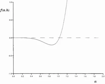
3.5 Plot of / ( a , h) against at with h = l... 61
3.6 Plot of Ci against a with h= 0.5... 62
3.7 Plot of Cr against a with h= 0.5... 62
3.8 Plot of / ( a , h) against a with h = 0.5... 62
3.9 Plot of Ci against a with h= 0.25... 63
3.10 Plot of Cr agednst a with h = 0.25... 63
3.11 Plot of / ( a , h) against a with h= 0.25... 63
3.12 Plot of Ci against a with h= 0.125... 64
L IS T OF FIGURES 7
3.14 Plot of f{a, h) against a with h = 0,125... 64
7.1 ^J5 > 0, AB > 0 and r = 0.01... 117
7.2 > 0, AB > 0 and T =0.2... 118
7.3 ^ B > 0, AB > 0 and r = 1... 118
7.4 A B > 0, AB > 0 and F = 6... 119
7.5 v4B > 0, AB > 0 and F = 10... 119
7.6 AB < 0, AB < 0 and F = 0.2... 120
7.7 A B < 0; AB < 0 and F = 1... 120
7.8 AB < 0, AB < 0 and F = 6... 121
7.9 AB < 0, AB < 0 and F = 10... 121
7.10 AB < 0, AB > 0 and F = 0.3... 123
7.11 AB < 0, AB > 0 and F = 1... 123
C hapter 1
In trod u ction
1.1
C lassical boundary layer theory
The foundations of classical boundary layer theory were laid by P ran d tl (1904) who addressed the flow of a fluid with small viscosity past a solid surface. In his paper on this subject, presented in 1904 at the Third International Congress of M athem aticians, P rand tl postulates the existence, between the main body of the flow and the solid surface, of a relatively thin viscous layer, the m otion of which is regulated by the pressure gradient in the inviscid m ainstream flow. W ithin this boundary layer the velocity increases smoothly but steeply from zero at the sohd surface to th e inviscid shp-velocity at the edge of the layer.
The physical problem resulting from these postulates gave rise to one of th e original, and now classical, solutions of boundary layer theory, the Blasius (1908) sim ilarity
solution. Here Blasius shows th a t the attached flow strategy can work in the case of an aligned flat plate immersed in a uniform stream .
C H A P T E R 1. IN T R O D U C T IO N 9
went on to dem onstrate the existence of the separation singularity, a reahzation which heralded the collapse of the attached flow strategy, it was his two-tiered structure which, in p art, m otivated the search for an alternative strategy which would produce regular separation.
The attached flow strategy of classical boundary layer theory is thus based on the following main assumptions:
1. The viscous effects are conflned mainly to a thin boundary layer lying close to the solid surface of a body and to a thin viscous wake.
2. The m ainstream flow is supposed unaffected by the presence of the bound ary layer and the boundary layer solution is constructed to correspond with the undisturbed m ainstream , in particular the pressure at any point in the boundary layer is th a t of the m ainstream at the same section.
Experience suggests th a t for m ost thick bodies these assumptions are unrealistic and th a t separation occurs, the boundary layer breaking away from the solid surface and forming a shear-layer downstream signiflcantly detached from the body.
At the onset of separation, accurate numerical solutions (Brown and Stewartson (1969)) of the boundary layer problem for flows w ith prescribed pressure gradients generally indicate the occurrence of the Goldstein (1948) separation singularity at the point of zero skin friction. This separation singularity, when encountered, cannot be sensibly removed using a shorter-scale analysis, as is shown by Stewartson (1970). Thus, with the exception of a few notable cases of which Blasius (1908) is one, the classical scheme described above never works.
C H A P T E R 1. IN T R O D U C T IO N 10
Neiland (1969), Messiter (1970), and predicts a triple-deck structure which holds on a shorter lengthscale 0 (Æe” ^/®) in the neighbourhood of the point of separation and is described in §1.2. See, for example, the reviews by Smith (1982) and (1986a), and the subsequent dem onstration of its application to instability theory. Smith (1979a,b).
We note here th a t there are two types of separation which can occur in boundary layer flows. The first is breakaway separation (or free separation) which is observed in flow past a bluff body. The second type may be described as local separation and occurs in flows past small humps, corners, injection slots, trailing edges, etc. The two types of separation are related, e.g. by the triple-deck structure (as described below), and are interactive with relative pressure unknown, hence avoiding th e Goldstein singularity.
1.2
T he triple-deck structure
On a lengthscale 0{Re~^/^) about the point of separation the adverse pressure gradient induced by the flow outside the boundary layer drives a reversed flow in a sublayer, or lower deck, close to the solid surface and of thickness 0 (i2 e “ ®/®). This causes a shear layer, or main deck, of thickness 0 { R e ~ ^ l‘^) to be pushed out into the m ainstream flow, which in tu rn modifies the adverse pressure gradient. A third region, or upper deck, is needed, but in the potential flow outside the boundary layer, to relate the induced pressure to the local displacement. Because potential flow is expected in this third region its thickness is comparable with its streamwise lengthscale 0 ( i2e"^/®).
C H A P T E R 1. IN T R O D U C T IO N 11
=
-^'w+S’
(:-')
w ith
U = V = 0 at
y
=o,
Î7 ~ y + A(^X'j as y —> oo, i U , V , P ' , A ' ) ^ { Y , 0 , 0 , 0 ) as X - > -o o .The unknown displacement increment —A { X ) is linked to the unknown induced pressure P by A ckeret’s law
P { X ) = - A \ X )
in the case of supersonic motion, and by the Cauchy-Hilbert integral
in th e case of subsonic motion.
However, triple-deck flows are observed to be often unstable in practice, see again Smith (1979a,b), and yield transition to turbulence; see following sections. It is this observation which forms p art of the motivation for the following study.
In overall term s this thesis is concerned with separating or near-separating two- dimensional basic flows, although the three-dimensional basic flow is touched upon in C hapter 4.
1.3
H ydrodynam ic stability
C H A P T E R 1. IN T R O D U C T IO N 12
im portance with regard to engineering, meteorology and oceanography, and astro physics and geophysics. It is concerned with when and how lam inar flows break down, their subsequent development and their eventual transition to turbulent flow.
Few authors on this subject have been able to introduce the concept of hydrodynamic stability w ithout seeking the assistance of Reynolds (1883) and his own description of his classic series of experiments on the instability of flow in a pipe.
The . . . experiments were made on three tubes — The diameters of these were nearly 1 inch, I inch and ^ inch. They were all . . . fitted with trumpet mouthpieces, so that water might enter without disturbance. The water was drawn through the tubes out of a large glass tank, in which the tubes were immersed, arrangements being made so that a streak or streaks of highly coloured water entered the tubes with the clear water.
The general results were as follows
1. When the velocities were sufficiently low, the streaks of colour extended in a beautiful straight line through the tube.
2. If the water in the tank had not quite settled to rest, at sufficiently low velocities, the streak would shift about the tube, but there was no appearance of sinuosity.
3. As the velocity was increased by small stages, at some point in the tube, always a considerable distance from the trumpet or intake, the colour band would all at once mix up with the surrounding water, and fill the rest of the tube with a mass of coloured water. Any increase in the velocity caused the point of break down to approach the trumpet, but with no velocities tried did it reach this. On viewing the tube by the light of an electric spark, the mass of colour resolved itself into a mass of more or less distinct curls, showing eddies.
C H A P T E R 1. IN T R O D U C T IO N 13
However,
the critical velocity was very sensitive to disturbance in the water before entering the tubes This at once suggested the idea that the condition might be one of instability for disturbances of a certain magnitude and stability for smaller disturbances.
At the critical velocity
another phenomenon . . . was the intermittent character of the disturbance. The disturbance would suddenly come on through a certain length of tube and pass away and then come on again, giving the appearance of flashes, and these flashes would often commence successively at one point in the pipe.
These ‘flashes’ are now known as turbulent spots, see for example Smith (1995). Below the critical Reynolds number the flow was of a lam inar Poiseuille form with a parabolic velocity profile. As the velocity was increased above its critical value Reynolds found th a t the flow became turbulent with a chaotic motion th a t strongly diffused the dye throughout the w ater in the tube.
Reynolds’ description illustrates the aims of the study of hydrodynamic stability: to determine w hether or not a given lam inar flow is unstable and, if it is, to investigate how it breaks down into turbulent or some other lam inar flow.
Since the subject of hydrodynamic stability is hugely varied in its application, and in the light of the work contained within this thesis, we restrict ourselves hereinafter to the subject of boundary layer stability and the subsequent transition to turbulence.
1.4
B oundary layer stability and transition to turbu
lence
C H A P T E R 1. IN T R O D U C T IO N 14
Schubauer and Skram stad (1947), and the much later work of Dovgal et al (1986). On the theoretical side the processes of transition form three m athem atically dis tinct levels or stages, namely Hnear disturbance theory, weakly nonlinear theory, and finally strongly nonlinear theory.
As is described in more detail in Chapter 2, the classical linear disturbance theory can be formulated by superimposing a disturbance on a given steady-state solution of the Navier-Stokes equations, resulting in the nonlinear Orr-Sommerfeld system of equations which governs the disturbance behaviour. Linearizing these equations for small disturbances, homogeneous equations are obtained which, when coupled w ith appropriate homogeneous boundary conditions, produce an eigenvalue problem for the grow th-rate param eter and hence determine the eflfect, stabilizing or de stabilizing, which the disturbance has on the basic fiow.
C H A P T E R 1. IN T R O D U C T IO N 15
By way of an example, and in reference to Chapter 6, we note here th a t the condition
:dy = 0, (1.3)
i
0 { U o - c o Yis a direct result of strongly nonlinear stability theory and is in accordance with Smith (1988), agreeing with experiments as shown in Smith and Bowles (1992).
Since th e development of triple-deck theory (see §1.2) over two decades ago, inter active descriptions of boundary layer flows have become a valuable tool in obtaining a greater theoretical understanding of both the transition process and, it is hoped, ultim ately a systematic account of turbulent flow and turbulence modeling.
Among those more widely used in the study of transition and turbulence in both incompressible and compressible boundary layers are, for example, viscous /inviscid, two-/ three-dimensional, small-/large-scale, and vortex/w ave interactions, see Smith (1993) for a detailed account of current research employing these interactions.
Our concern within the la tte r chapters of this thesis is with nonlinear vortex/wave interactions initiated within an interactive boundary layer, following on from a string of papers on vortex/w ave interactions by Hall and Smith (1988, 1989, 1990, 1991), Brown et al (1993), Smith et al (1993) and more recently Timoshin and Smith (1995), Brown and Smith (1995); much of Chapters 5 and 6 is based upon Smith et al (1993). A separate and approximately simultaneous string of papers is by Benney and Chow (1989), Goldstein and Choi (1989), Wu (1993), Wu et al (1993) and Khokhlov (1994), including non-equilibrium critical layers which have an extra effect (time-dependence) acting in the critical layer but miss the nonparallel flow effect th a t is present in Smith et al (1993) [later referred to as SBB].
C H A P T E R 1. IN T R O D U C T IO N 16
1.5 V ortex/w a ve interactions
Vortex/wave interactions arise in various forms, principally with either viscous- inviscid ToLLmien-Schlichting waves or inviscid, inflectional Rayleigh-waves; see again Hall and Smith (1991), Brown et al (1993), Smith et al (1993). A feature common to all such interactions is th a t at high Reynolds numbers three-dimensional waves are coupled nonlinearly with the mean flow via its unknown longitudinal vortex component.
This coupling is term ed weakly nonlinear if the vortex p art is a small-amplitude perturbation of the mean flow. On the other hand, the coupling is strongly nonlinear if the mean flow comprises entirely the vortex contribution, as in the flow considered in the la tte r chapters of this thesis.
The work of Hall and Smith (1988, 1989, 1990, 1991) in particular highlights the ability of vortex/wave interactions to provoke strongly nonlinear effects even for extremely small three-dimensional input disturbances.
It has been noted in Brown and Smith (1995) th a t an obvious reason for the the oretical focus on vortex/wave interactions is the qualitative and quantitative links w ith experiments on transition described by Hall and Smith (1991), W alton and Smith (1992), Stewart and Smith (1992) and Smith and Bowles (1992) for a variety of input conditions. It is also noted th a t observations of the significant role of longi tudinal vortices in the early stages of some transition paths are given experimentally by Klebanoff and Tidstrom (1959), Nishioka et al (1979) and others.
1.6
D escrip tion o f subsequent chapters
C H A P T E R 1. IN T R O D U C T IO N 17
number interactive boundary layer flow is investigated downstream of tbe point at which th e boundary layer itself separates away from the wall. Initially the point of interest is sufficiently far downstream th a t we can ignore the presence of the wall, thus assuming the extent of the flow is inflnite both above and below the separating boundary layer. In steps we move our point of interest upstream , always remaining outside the interactive triple-deck region, introducing the etfects of the wall via appropriate boundary conditions. At each step the disturbances within the boundary layer are governed by the Rayleigh equation and we emphasize the structures and scales involved which, together w ith the solution obtained, determine the structures and scales of subsequent steps. N eutral eigensolutions are considered and the value of the wavenumber obtained to leading order. A critical distance downstream of separation is found at which the disturbance characteristics alter rapidly.
Continuing on from the work of C hapter 2, in C hapter 3 we consider the linear stabil ity of the basic flow to long-wave inviscid perturbations. Here we also dem onstrate, by comparison, the value of modeling the basic velocity profile using a piecewise- linear approxim ation which possesses some of the m ain features of the basic flow.
C hapter 4 provides a possible link between the linear studies of Chapters 2-3 and the nonlinear work to follow in Chapters 5-7. Here we are concerned w ith the Rayleigh instabilities which occur in separating two- and three-dimensional boundary layer flows as a result of inflectional velocity profiles produced locally, for example, flows past humps, corners, injection slots, trailing edges etc. Experim ental studies of flow transition over various isolated or distributed roughnesses on solid surfaces are given in Acarlar and Smith (1987) and references therein, while com putational studies include Mason and M orton (1987) and other works.
C H A P T E R L IN T R O D U C T IO N 18
inflectional point in the local velocity profile is a necessary but not sufficient con dition for Rayleigh instability. Based on this paper, we show th a t as the boundary layer undergoes increased separation, i.e. the inflectional point moves upwards in the positive y-direction, a cut-off point exists at which the flow ceases to be un stable. Moreover, this point occurs prior to the point at which the inflection point itself leaves the lower deck, re-iterating the findings of Smith and Bodonyi (1985).
A detailed description of the work of Smith et al (1993) [SBB] is presented in Chap te r 5 in which the starting process of strongly nonlinear vortex/Rayleigh-wave in teractions in a boundary layer is considered on a shorter lengthscale than th a t of Hall and Smith (1991), Brown et al (1993). On this new shorter lengthscale the ab rupt starting of the interaction is smoothed out and the wave-pressure am plitude no longer satisfies the bifurcation equation of the previous works, now replaced by an integro-differential equation. Here, however, we restrict ourselves to a boundary layer of interactive triple-deck form, the scales involved proving significant in later chapters.
In the la tte r sections of this chapter, and in preparation for the following chapter, we introduce the additional influence of a slow time derivative dt^ accompanying the slow spatial derivative dx^ •
The starting point for C hapter 6 is the integro-differential equation obtained in SBB, and derived again in the previous chapter, in which the wavenumbers a and are taken to be 0 (1 ). Here we let a , P —>0 and consider the solution in the core region of the flow, deducing th a t
7 = 2/ f{y)l{ÿ)dÿ, (1.4)
C H A P T E R 1. IN T R O D U C T IO N 19
where
7" =
1(5) = f \ U o - c o ) - ^ d y .
J0 0
Given the wave speed and the basic velocity profile we may conclude th a t (1.4) fixes the value of 7 at leading order before the wave-pressure am plitude (integro- differential) equation can come into play at second order. Fixing 7 in tu rn fixes the input frequency fi, thus restricting the range of frequencies to which the vortex/w ave interaction theory of SBB apphes.
By considering certain physical characteristics of the flow we set up an entirely new regime in which a = 0{Re~^^^^) and the streamwise lengthscale is shortened still further. The wave-pressure amplitude equation thus obtained comprises the integro- differential equation of Chapter 5 and (1.4), now acting together at leading order. This new equation holds for arbitrary input frequencies 0 , further generalizing the application of vortex/Rayleigh-wave interactions in interactive boundary layer flows. A lternative regimes are briefly discussed, highlighting their physical im portance and m athem atical consequences.
C H A P T E R 1. IN T R O D U C T IO N 20
Work is in progress with Professor F T Smith to investigate in more detail the im pact of th e initial-value problem on weakly nonlinear theory.
C hapter 7 presents numerical solutions of the integro-differential equation when the effects of forcing are taken into account, corresponding to a nonlinear receptivity problem. Comparisons are made with the numerical solutions of SBB, the case of no added forcing, to establish the effects of the forcing downstream of its point of application.
The main novel contributions of this thesis are perhaps threefold, namely:
1. The account in Chapters 2-3 of the behaviour of neutral wavenumbers in the separating boundary layer flow downstream as it detaches from the wall.
2. The inclusion of tem poral effects in the nonlinear vortex/wave interactions at the onset of inflectional instability, leading to the new initial-value problem there (C hapters 5-6).
3. The nonlinear forced vortex/wave interaction solution properties of C hapter 7.
C hapter 2
Linear stab ility o f a
tw o-dim ensional separating
in teractive boundary layer
2.1
Introduction
Because of the m athem atical simplifications associated with linearization and the fact th a t linearized theory is able to provide the critical conditions for the occur rence of instability for infinitesimal disturbances, stability theory has largely been developed w ith this restriction. However, in recent years the role of nonlinearity in flow instability has received increasing study, see for example the work of Stew art son and S tuart (1971), Smith (1979b) and Hall and Smith (1991), consideration of which is the eventual aim with regard to the present thesis. Thus, the present work considers linear properties first, followed by certain nonlinear aspects in the later chapters.
The m athem atical problem of hydrodynamic stability can be formulated by taking th e given steady-state solution to the Navier-Stokes equations and superimposing a
C H A P T E R 2. L IN E A R S T A B I L I T Y T H E O R Y 22
disturbance of a suitable kind. The result is a set of nonlinear ‘disturbance’ equations governing the behaviour of the disturbance. If the disturbance ultim ately decays to zero the flow is said to be stable. On the other hajid, if the resulting disturbance is perm anently nonzero the flow is said to have become unstable. On Hnearizing these equations for small disturbances homogeneous equations are obtained, allowing dis turbances which contain an exponential time factor of the form e®* to be considered, t denoting time. Along with homogeneous boundary conditions the result is an eigenvalue problem for the determ ination of q, th e grow th-rate param eter th a t in dicates the effect, stabilizing or de-stabilizing, which the superimposed disturbance has on the basic flow.
In this chapter the growth of hnear disturbances in a high Reynolds number interac tive boundary layer flow is investigated, the flow being considered beyond the point at which the boundary layer separates away from a smooth wall. The disturbances within the boundary layer respond according to the Rayleigh equation, considered here for neutral-wave solutions, and in each case the structure and scales of the instabihty are presented. In considering the neutral-wave solution three regimes are examined. Initially the flow is examined far downstream of the point of separation where the effects of the wall are assumed neghgible, the flow being taken to be in flnite both above and below the separated boundary layer. Moving back towards the point of separation, a second regime is considered in which the presence of the wall becomes im portant. It is the results obtained here which lead the investigation into th e final regime, ju st beyond the point at which separation occurs, where the typical y-scaling of the small disturbance is seen to increase.
C H A P T E R 2. L IN E A R S T A B I L I T Y T H E O R Y 23
separation” should be taken to mean just outside the 0 (iEe“ ^/®) triple-deck region.
The strategy adopted here is similar to th a t of Papageorgiou and Smith (1989) in which two-dimensional stability theory is applied to a waJte formed ju st dow nstream of a flat plate. In §2.2 below the linear stability problem is form ulated. In §2.3 the structu re and scales are described and the Goldstein-type velocity proflles, which hold beyond the triple-deck region, aje given. Neutral-wave solutions are found in §2.4 for each of the regimes outlined above and the changes in the disturbance structure and scales of the flow are set out accordingly. By way of a check, §2.5 presents and compares the results of a numerical calculation carried out in support of th e analysis obtained in the third and final regime of §2.4. In §2.6 the neutral curve is presented in full and concluding remarks then follow.
Throughout this chapter in nondimensional term s the origin of the Cartesian coordi nates is fixed at the point of separation xq, with x , y the streamwise and transverse coordinates respectively. In addition u , v , p are the velocities in the z-direction, the
1/-direction and the pressure respectively, and tp denotes the stream function for the two-dimensional flow.
2.2
Form ulation o f th e linear stab ility problem
Beyond the point of separation the boundary layer experiences a gradual shift away from the smooth wall. The thickness of the boundary layer remains of order Re~^!'^ and th e motion is governed downstream by the two-dimensional boundary layer equations.
C H A P T E R 2. L IN E A R S T A B I L I T Y T H E O R Y 24
and thus the prime scales are x ~ y ~ Re~^^^. The two-dimensional unsteady Navier-Stokes equations form the basis of the problem and the basic flow at a flxed X-station is two-dimensional and quasi-parallel, w ritten as (ü(y), 0) to leading order. Linearization about the basic state reduces these equations to
du _d u dû dp 1 .d^u d^u
dv _ d v dp 1 .d^v d^v.
du dv
"5— ^ dx dy — O'
However, assuming th a t the Reynolds number is asymptotically large the effects of viscosity are neglected and the Navier-Stokes equations become
du du dû dp
dv _ dv dp
+ = - % '
ë + S = °
(2.1)in the classical Rayleigh fashion (e.g. see S tuart (1963)).
It is convenient to define
d(f> ,
where th e stream function ip is given by '^(x, y, t) = (j){y) e x p [ia (x -c t)]. The quantity a is real and is the wavenumber of the disturbance in the x-direction. On the other hand, c is complex; the real p art, namely c^, is the wave velocity and the im aginary p art, namely c%, represents the amplification or damping of th e oscillation w ith time. If Ci is positive the disturbance amplifies and becomes unstable, while if it is negative the disturbance decays and is stable. The situation of neutral stability is governed by Ci = 0.
C H A P T E R 2. L IN E A R S T A B I L I T Y T H E O R Y 25
(ü - — a^(f>) = v!'(j)^
with, (j) required to vanish at the wall and as y —^ oo in the freestream.
A n extremely importéint result obtained by Rayleigh (1880) is th a t a necessary condition for instability in an inviscid fluid is th a t the velocity profile ü should contain a point of inflection. ToUmien (1935) has since shown th a t for symmetrical velocity profiles in a channel, and boundary layer velocity profiles, the condition u" = 0 is also a sufficient condition for instability. In some other contexts however it is not sufficient: see Chapter 4.
2.3
Stru ctu res and scales
In considering th e possibility of neutral eigensolutions ju st beyond the point of separation xq the basic velocity profile must be examined more closely and its points of inflection found. If the given profile ü has an inflection point at y = j/, say, then for sym m etrical profiles in a channel and boundary layer profiles there is a band of wavelengths a (< a ,) for which Q > 0, giving instability, and this band is bounded by the neu tral state
(pg — ^(y^)) ol — OLg 0, c — u(yg) = C5, Ci —0. (^'^)
The profile used is th a t just beyond the triple-deck region of the separation and is described below.
For y = 0 ( 1 ) ü = ü{y), where
ü ~ Ay - + £7 + . . . (2.3)
C H A P T E R 2. L IN E A R S T A B I L I T Y T H E O R Y 26
For y = ez, z = 0 (1 ), ü = 6F (z), where the Goldstein-like function F{z) is such th a t
F { z ) ~ Xz -(- Aq - f - ^ e 9^ -f ... ( 2 .4 )
as z —> 00 and F { z ) —> 0 as z —> —oo.
Here e = (x — 7 is a positive constant and Aq is a Goldstein displacement
constant. We may locate the inflection point by combining (2.3) and (2.4) and balancing their second derivatives. This yields an inflection point at y = eX -f 0 (e ) where L^ = —(9/;^loge. From (2.2), combined with (2.3), we see th a t the neutral wave speed has the expansion
c = eXA e^X^c , (2.5)
and a balance of terms in the Rayleigh equation leads to the following expansion for a;
OL — — Y “t" 0 :1 eXo'2 . ( 2 . 6 )
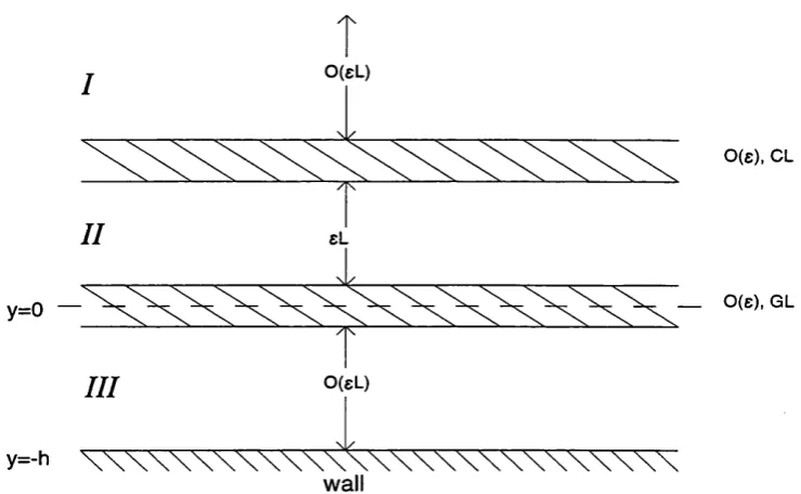
Solutions must be found in each of the regions shown in Figure 2.1 and matched w ith those of neighbouring regions.
2.4
N eutral-w ave solutions
Initially in w hat follows we consider the problem set out in §2.3 for the case in which the presence of the wall is ignored, i.e. the flow is considered far enough downstream of th e point of separation xq for the effect of the wall to become negligible. Thus the extent of the flow is assumed infinite both above and below the separating boundary layer and boundary conditions are apphed accordingly.
C H A P T E R 2, L IN E A R S T A B IL IT Y TH E O R Y 27
O(eL)
0(e). CL
y=0
O(eL)
III
y=-h
— 0(E), GL
wall
Figure 2.1: The various regions in which neutral waves develop. CL denotes the critical layer, GL the Goldstein layer.
presence of the wall. Thus, through the new boundary conditions, we introduce the separation distance h between the boundary layer and the wall. It is the results obtained for this case which lead us into the second and third regimes, moving our position of interest upstream towards the point of separation by reducing h gradually.
C H A P T E R 2. L IN E A R S T A B IL IT Y T H E O R Y 28
2 .4 .1 R e g im e 1
R eg io n I
We begin in region I in which y = eL (l + Y ) , 0 < Y = 0 (1 ), and the expansions for Ü and (j> are
Ü = e L \ { l + y ) - e^A2i ^ ( l -}- Y Ÿ + ^2^4(1 + Y Y ^ ^ + • • • j (2 7) (f> — (f>o“f" ^L(f>\+ L^(j) 2 + . . . , (2.8)
where E j = exp[—(A/9)Z-^(1 + Y)^].
S ubstituting (2.5) - (2.8) into the Rayleigh equation and balancing successive powers of eLj we obtain the equations
A y ( ÿ g - a g ÿ o ) = 0, (2.9)
\ Y — o^(j>i — 2(XoOii<t>o) — —2A,^o, (2.10)
subject to the boundary conditions —» 0 and ► 0 as Y oo. It should be noted here th a t for (2.9) and (2.10) to hold true we require th a t
be small compared with e~^L~^ and be small compared w ith 1. Since Y > 0 in region I these requirements are met and therefore the first and second order term s in the expansion of (f> have solutions
ÿo = A oe-“”^ , (2.11)
- a i A o Y e - " ^ ^ + ^ ^ e - ““^ l o g y
olqX
, ^ Y
A&Ao -e
0-0 A (2.12)
where Ao, B \ are constants. In order to achieve our goal it is necessary only to obtain a solution for the first two term s in the expansion for (f) in region I.
It can be shown th a t as Y —^0+
C H A P T E R 2. L IN E A R S T A B IL IT Y T H E O R Y 29
where Dq, D2 are constants and D2 = —2A2A0/A.
We will use (2.13) to m atch the solution of region I with th a t of the critical layer, which we now proceed to obtain.
C ritical layer
Here y = eL -\- ez ( —00 < z <00) and, since Y = zL~^, the expansions for ü and 4> impHed in the critical layer are
Ü = eZ-A + eAz — e^Zr^A2( l + ^)^-|-eZ ^ + . . , , (2.14) (j>= fpo+ Z ^“01 + Z ^*02 + . . . + eZ "I"00 4- Z + .. .^ + . . .
+ L (2.15)
where Ec l = ex p [-(A /9 )Z ^ (l + zL'^Ÿ].
Substituting expansions (2.5), (2.6), (2.14) and (2.15) into the Rayleigh equation we obtain the equations
\ ziI)q = 0, AzV»i = 0, Az(-02 - ckqV'o) = 0, (2.16)
and
Az-^o = 0, Az*^" = —2A2'0o- (2.17)
The solutions of (2.16) consistent with those in region I are
-00 = ^0, V’l = - olqAqz, ^2 = \ a l A o z ^ .
In order to m atch with the solution in region I it follows from (2.17) th a t -0o = Dq
while the equation for becomes
C H A P T E R 2. LIN E A R S T A B IL IT Y T H E O R Y 30
Again, on matching with the solution in region I we have
7 2AgAo, , \ I L
V’l = T— ( z l o g z - z) + biz
where bi = Di —2A2A0/A. Finally the equation for is obtained from a balance of term s 0 { e ~ ^ jE c L ) in the Rayleigh equation and is
V’o =
R eg io n II
Continuing into region II where y = eL{l + Y), — 1 < Y" < 0, the effects of the exponential term in the basic velocity profile must be considered more closely. Here th e expansions for ü and <f> axe
Û = e L \ ( l + Y ) - + Y f + + . . . , (2.18)
(i+y)®
(f> = (l>o + ^L(f>\ + . . . + !/ ^ ^ 1^0 + 1^ + • • - j- + • • • 5 (2.19)
where E j i = e x p [-(A /9 )ü ^ (l + y)^].
In (2.19) 00 is given by (2.11) and 0 i satisfies (2.10). We note here for future reference th a t at the Rayleigh equation implies
which matches with the contribution from 00 in the critical layer.
G o ld ste in layer
Moving into the Goldstein layer where y = ez, z = 0 (1 ), and ü = eF (z), 0 has an expansion of the form
C H A P T E R 2. L IN E A R S T A B IL IT Y T H E O R Y 31
On substituting (2.5), (2.6) and (2.20) into the Rayleigh equation, along w ith the above expression for ü, we obtain
= 0, - A $ ï = F"{z)^o- (2.21)
In matching w ith region II it follows from (2.21) th a t $o = Aoe°^° while the equation for $1, along with its behaviour as z —^ oo, is
$1 = --- ^— F (z ) + clqz + bo, (2.22)
$1 ^ --- ^— (Az + i4.G + ) + uqz + 6q. (2.23)
The exponential term in (2.23) matches with the contribution from of region II as Y —» — 1"^. As there is no constant term of order L~^ in the solution for <f> obtained in region II, we may deduce th a t bo = AoAcA'^e^o. In order to determine the value of ao, and hence ao, it is necessary to m atch the solution across the Goldstein layer into region III.
R eg io n III
In region III y = e L Y for Y < — 1 and the basic velocity profile ü is approxim ated to zero. The expansion for (j) is now
(f) — (j>o L ^(j)oi + . . . + eT {^1 + ...} + . . . . (2.24)
In (2.24) 4>o satisfies (2.9) subject to the boundary condition th a t 0 as T —oo and therefore <f>o = Aoe“°^, where Ao is a constant to be determined. Sim ilarly,
<Aoi - Q!o<^oi = 0 (2.25)
C H A P T E R 2. L IN E A R S T A B IL IT Y T H E O R Y 32
M atching into the Goldstein layer it follows th a t
Âo = Aoe^°‘°, Â i = AoAc^~^e^°‘°, ao = aoAoe°‘°. (2.26)
Finally, matching the linear terms of order L~^ across the Goldstein layer, a value for 0=0 is obtained, namely
ao = - , (2.27)
implying a neutral wave frequency u; = ac = j O(eL). The results above indicate th a t when the the presence of the wall is ignored, typical wavelengths for neutral waves are O(eL).
We m ust now introduce the effects of the wall on th e flow as our position of interest X starts to move back upstream towards the point of separation, still remaining outside the triple-deck region. At this early stage these effects are seen only in region III in which the boundary condition to be satisfied by the stream function reduces to the requirement th a t ^ = 0 at y = —h. M atching similar to th a t above yields th e result
^ “ t a n h l o S
where h = eLH. Notice th a t as Æ —» oo, i.e. as the current position progresses dow nstream , (2.28) becomes ao ~ 1 — ao &nd so we regain the result (2.27) in which the value of H was effectively taken to be infinite.
W ith (2.28) as our starting point we now begin a closer exam ination of the separation distance H and its effects on the value of the resulting wavenumber a to leading order. If we let H 0"^ in such a way th a t aoH —> O'*" it follows th a t
ao ~ 1 — - 1
C H A P T E R 2. L IN E A R S T A B IL IT Y T H E O R Y 33
/[\
O (G L ')
) e
-O(eL)
II
y=0
y=-h
0(6), GL
wall
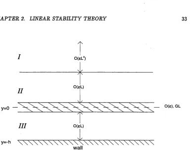
Figure 2.2: The flow structure at .E-values close to the critical value He, y = eLH.
2.4.2
R egim e 2
The analysis carried out in Regime 1 above indicates the need for a more detailed investigation into the effects of the separation distance h on the boundary layer flow under consideration, in particular on the wavenumber a , about th e point at which the scaled separation distance H attains the critical value of 1. As mentioned above, at this value the wavenumber vanishes to leading order and so it is necessary to consider the behaviour at second order, achieved by expanding H about its critical value. We write
H = 1 L -f-. . .
implying an expansion for the wavenumber a of the form
O' = e ^ L ^0=00 "t“ ( ^ L ^oiQi + • • • + 0:10 4- L + O(eZr). (2.29)
C H A P T E R 2. L IN E A R S T A B IL IT Y T H E O R Y 34
will use m atched asym ptotic expansions to solve the Rayleigh equation, noting th a t in these regions it reduces to the equation
for the order of working considered, i.e. the — t er m may be neglected. If in (2.30) we write (j) in the form
<f> = ( Ü - c)f{y ) (2.31)
for some function f{ y ) , we obtain the integral equation y
= D i{u - c )
J { u -
c)-^d t (2.32)Vw
»/,
where y ^ = eLq, q = and D i is some constant to be determined. This can be rew ritten in the form
A D
Solving (2.33) directly will provide us with an alternative form of the required solu tion and may be used to determine the value of arbitrary constants obtained using th e m atched-asym ptotics approach.
In w hat follows, the process of solution begins in those regions closest to the smooth wall itself and proceeds in the ‘upw ard’ direction of y increasing, towards the m ain stream flow.
R eg io n III
Here y = eL Y , —H < Y < 0 , the basic velocity profile û is approxim ated to zero and the expansion for <f> takes the form
C H A P T E R 2. L IN E A R S T A B IL IT Y T H E O R Y 35
A balance of similarly-ordered term s in the Rayleigh equation yields
-X(j>oo = 0, -\<Poi
=
0,—A0O2 + Aago^oo = Oj "^^0 3 + + 2Aa=oo 0=01^00 = 0,
and
-A<^"o = 0, —A^ii -j- 2AaooQ!io^oo = 0,
^12 "b 2A {0:000:11 + o:oiO:io} <Poo + 2Ao:ooO:io^oi + ^ckqo^io = 0,
which have solutions of the form
000 = AqY Bq,
001 = CqY - f Dq,
002 = 20:00 I -^Oj
003 = gO:QQ I 2 ^ 0 ^ ^ + D o l^ ^ j + 0:000:01 ^ + GqY + Hq,
and
010 = ÂqY H" Èq,
C H A P T E R 2. L IN E A R S T A B IL IT Y TH E O R Y 36
Applying the boundary condition (^ = 0 at the wall we find th a t
Ao = Bo, Dq = C o + A o h ,
Coh = ûqoAo/S — Eq + i^o, Âo = Bo,
D q = C o + À o h — 2aoo<^ioAo/3.
Since ü ~ 0 in region III, it follows from (2.33) th a t the solution to the reduced Rayleigh equation taking the form of (2.31) is
(f)6 11 l1 ^ c f l 1 1
>1
''J-.L-ek
c 2 ( A t-D i J-eL-eh. (At — c)^ A | (eBY — c) (AeB + e^B^Ah + c) j * (2.35)
where, as before, c is given by (2.5). Matching this solution with th a t obtained using the m ethod of asymptotic expansions we deduce th a t D \ = — AAq, Co = 0
and Ao = —cA~^Ao, Ao remaining arbitrary.
G o ld stein layer
Inside the Goldstein layer y = ez, ü = eF{z) and the following expansion is implied for <f)]
<f> = $ 0 4" L ^$1 + . . . + eB($o 4" B 4~ • • •) 4~ • • • • (2.36)
In order to m atch with the solution in region III as 2 —»• — oo, we note here th a t in this limit the term s of (2.36) are such th a t
$ 0 ~ Ao,
$1 ~ Aoz + Aoh,
$2 ~ Bo,
$ 3 ru (Bq -0:QQAo)z + Ho,
1 2
C H A P T E R 2. L IN E A R S T A B IL IT Y T H E O R Y 37
and
cAo A ’
$1 ~ + A) — —OiooQiio-^o + Cq. (2,38) Substituting (2.36) into the Rayleigh equation, with a given by (2.29), c given by (2.5) and ü = eF{x), we obtain
= 0,
- A $ ï = y % z)$ o ,
- A $ ; + = F " ( z ) $ i, (2.39) - A $ ï + F ( z ) $ ; = y % z ) $2,
- A $ ï + F ( z ) $ ï + Aago$o = F ' \ z ) ^ s . and
-A#% = 0,
- A $ ï - c0" = F "(z )$ o . (2.40) The solutions of (2.39) which satisfy the conditions of matching with region III, as set out in (2.37), are
$ 0 = -4.0, $1 = —— F{z) + Aq(^z + A),
$2 = {^F {z) — 27i(z)} — -^ F {z ) -f Fq,
$ 3 = — 2i4o
“Â ^ ^ F { z ) Ii { z ) - - 7 2 ( 2 ) | — + 2^00^0)2 + ^ 0,
$ 4 = ^F {z)l2 {z) - -73(2) j - - ( 7 b + gCKoo^o) {zF {z) - 27i(z)}
— —^ F { z ) + - olqqAq z^ + —A o [ a Q Q h + aooctoi)^ + { H o — FqK )z + TTo,
(2.41)
where
7i (2) = f F{s) ds,
C H A P T E R 2. L IN E A R S T A B IL IT Y T H E O R Y 38
l2(z) = r F(s)^d3,
J—oo
h { z ) = r F { s f d s . J—oo
The solutions of (2.40), consistent with (2.38), are
« cAq
$ 0
-
.
4 i = ——^ F { z ) — — + h) — —0:000:10^0 + C^. (2.42)
Although not outlined here, given th a t D i = —XAq the alternative approach to solving the Rayleigh equation described in (2.30) - (2.33) also yields (2.41) and (2.42).
R eg io n II
Here y = e L Y , Y > 0, and the appropriate expansions for û and 0 are
U = e L Y - + eA c + + ■ • •. (2.43)
(j> = 4>o L 4- L ^<l>2 + . . . + e i ^^0 + R + .. .^ + . . .
+ L ^ 4- L ^ f i + eL ^ /o 4- L ^ f i 4 - .. .^ 4 - .. .^ 4 - . . . . (2.44)
From the Rayleigh equation we obtain as the equations for ^o, and (j>2
A (y - i)ÿ g = 0, A ( y - i ) ÿ ( ' = o, A ( y - i ) ( ÿ ; - a g ( , A ÿ o ) = o
which, in order to m atch with the Goldstein layer as Y —♦•O'*', have solutions
(f>o = ^0, = ^ o ( - ^ — ^ ) ( ^ — 1))
4-C H A P T E R 2. L IN E A R S T A B IL IT Y T H E O R Y 39
It can also be deduced from the Rayleigh equation th a t
Y *fo =
A ( y - I ) ’
y ’ / i =4j. AqAg AqAg AqAg A2 A 2 ( y - 1 )2 A ’
4 AqA}. AqAq Fq Q-oqAqY (1 11
^ 1 2 ^3 _ 1)3 A (y - 1) A (y - 1) 12 3 J '
m atching with the solution in the Goldstein layer as y O'*'. The governing equation for 0o is obtained from a balance of 0 (1 ) term s in the Rayleigh equation and is, together with its solution which satisfies matching requirements w ith the Goldstein layer,
2X2(f>o
A ( y - i ) '
^0 = - 2^ { ( y - i)io g |y - 1| - y } + £ ^ ( y - i) .
We note here for future reference th a t as y oo
^ ~ Ao + ( y — 1) + 0 ( lf ^,eZf), (2.45)
where only the term s given exphcitly are necessary in matching region II with region I for th e purpose of obtaining aoQ.
R eg io n I
In region I we introduce the new coordinate ^ > 0 such th a t
y =
w ith ^ = 0 (1 ). Here it follows th a t û and (f> have expansions of the form
C H A P T E R 2. L IN E A R S T A B IL IT Y T H E O R Y 40
and, when balances between term s in the Rayleigh equation are set up, the equation obtained for th e leading component of <f) is
- aS oto) = 0.
Hence $o = where A% is a constant. Matching this solution w ith th a t obtained in region II leads us to the result th a t A i = Aq. We notice th a t as ^ » 0"""
^ 0 ~ -^0 | l ~ 0=00^ + 2*^00^^ — .. • (2.48)
and, since Y L ^ for large Y and small on matching (2.45) with (2.48) we deduce th a t
I
d'oc = h. —.
The value obtained here for aoo provides the motivation for the third and final regime. By putting h = Ag^~^ in the expansion for H of Regime 2 we are able to conduct an even closer examination of the behaviour of the wavenumber aoo about th e point at which H attains its critical value of 1.
2.4.3
R eg im e 3
In the light of the results obtained in the working of Regime 2 we expand H in the form
H = 1 -]— 4" €Lh+ . . .
JjX
so th a t to leading order the wavenumber a is 0 (1), thus indicating the possibility of neutral waves of wavelength 0 (1 ) close to the point of separation. We w rite
a = a + Zf ^a% + L ^ct2 4 - .. . 4- cLÇâo + L ^0% + . .. ) + ...}
C H A P T E R 2. L IN E A R S T A B IL IT Y T H E O R Y 41
Similar m atching of the solutions in each of the flow regions I, II, III and the Gold stein layer leads to the eigenvalue problem
û((^S - (2.49)
for â , the 0 (1 ) equation obtained from the Rayleigh equation in region I, where as 3 / - .0 +
Û ~ Ay - ^2y^ +
00 ~ ^ 0 - Ao(h - j ) y - (y lo g y - y) + ^â^Aoy^
+ - ^)y2 + ^ ^ ^ ( y ^ l o g y - 3y^} + . . . (2.50)
in order to m atch with the solution obtained in region II.
We consider the problem presented in (2.49) and (2.50) for small wavenumbers and approach it b oth analytically and numerically, the analytical m ethod being described below.
The flow is considered in an outer region Iq in which y = â~^ÿ, ÿ = 0 (1 ) and û 1. The expansion for 0q takes the form
00 = 5 " ^ $0 + $1 + 0 $ 2 + . -,
and on substituting this into (2.49) we find th a t for % = 0 , 1 ,2 , .. .
= 0, $i = ai€~^, (2.51)
where each a» is a constant.
Moving into region I in which y = 0 (1 ), the behaviour of ü is such th a t
u ~ 1 as y —» oo,
Ü ~ Ay - A2y^ + O(y^) as y -> 0+
C H A P T E R 2. L IN E A R S T A B IL IT Y T H E O R Y 42
and it emerges th a t th e expansion for (j)o takes the form
<f>0 = ÔL ^^0 + ^1 + ÔL^2 + ^3 + • • • •
S ubstituting this expansion into (2.49) and equating powers of â yields the following equations for the four leading term s in (f>o]
= ü"^o, (2.53)
û^'l = ü"^i^ (2.54)
ü^2 — ^^0 = ^"^2^ (2.55)
- ü ^ i = ü"4>3. (2.56)
Considering equation (2.54) first, a possible solution for is y
<^i = &ii2 + 6ofi
J
û~^dyi, (2.57) 1where 6q &nd 6i are constants to be determined.
As 3/ —> oo, 01 behaves linearly with
01 ~ &i + boK, + 6oy> fOO
K = y- vT'^dy.
M atching w ith the solution obtained in region Iq as ÿ —> 0 we may deduce th a t
bo = - a o , bi oc 6q. (2.58)
As y ^ O'*" it can be shown th a t
7 bo 260A2 . , \
C H A P T E R 2. L IN E A R S T A B IL IT Y T H E O R Y 43
and therefore, to m atch with region II, it follows from (2.50) th a t bo = —-AqA, i.e. ao = Av4o.
The solution to (2.53) which matches with th a t of region Iq is
— CLqU — y^A-oiL.
To conclude we note th a t, in matching the solutions between regions I and II,
^0 ~ AALo 'IAt/ — A2%/^ + .. .|^ (2.59)
as 2/ —> 0.
If we assume th a t h — cX~^ is 0 (â ~ ^ ) then in matching with region II it follows from (2.59) th a t
h - c X ~ ^ = - A ^ d - \
Thus, to complete the neutral curve for the separating interactive boundary layer flow under consideration, aU th a t remains is for us to reinforce the assum ption made above, namely
h — ^ = 0(^ct ^). (2.60)
To do this we now solve numerically the eigenvalue problem set out in (2.49) and (2.50) for small wavenumbers.
2.5
N um erical solution o f R egim e 3
C H A P T E R 2. L IN E A R S T A B IL IT Y T H E O R Y 44
The numerical problem is thus. For a given wavenumber, â to leading, the value of the constant A i is to be found such th a t
(^o(O) = A i,
subject to the boundary condition th a t 0 as 3/ oo.
The undisturbed flow ü(y) is assumed to have exponential decay as 3/ 00; more precisely ü ~ 1 — e“ ^. For clarity, this model, rath er than the full Blasius profile, has been assumed to apply over all y since the effect of the decay is qualitatively the same.
The numerical m ethod of integration employed is the classical R unge-K utta m ethod of order four generalized to solve a system of first order differential equations, in this case a system of two.
The second order differential equation which arises from (2.49) and (2.50) is
(1 — e ^){(f)Q — â^(j)o) = —e ^0 0) (2.61)
subject to the initial and boundary conditions
<Ao(0) = Ao,
(^o(O) = A i, (f>o{oo) = 0.
W ith v{y) = (j>o{y) and w{y) = <j>o{y), (2.61) is transform ed into the system
v' = + (1 — (2,62)
w' = V, (2.63)
C H A P T E R 2. L IN E A R S T A B IL IT Y T H E O R Y 45
The range of dependence is taken to be y G (0,î/oo]j Voo a suitably large number. We then map this range onto the interval (0,1] using the transform ation y = f ( ÿ )
for 3/ G (0,1] where
If ÿ is taken over the range [ÿo, 1], where 0 < ÿo < 1? the system of first order differential equations in (2.62) - (2.63) becomes
w ith initial conditions w(ÿo) = 1, v(ÿo) = vq.
The interval [ÿo, 1] is divided into N equal subintervals, the transform ation y = f ( ÿ )
therefore concentrating the mesh points in the lower half of the interval [ f ( ÿo) , / ( I ) ] in which the stream function varies more dramatically. The differential equations (2.65) and (2.66) are used to obtain the value vq for different values of the param eter â, the tru e value taken to be th a t which results in the solution for 0o satisfying the appropriate boundary condition at yoo’, namely th a t (j>o{yoo) = 0 where y^o = / ( I ) -In the model described above the constants Aq, A and A2 take the values 1, 1, 0.5 respectively and therefore from equation (2.50) it follows th a t as y ^ O'*"
(f>o 1 - Ahy - {ylogy - y) + (2.67)
(j)Q ~ —Ah — log 3/ + . . . , (2.6 8)
where Ah = h — c \ ^.
C H A P T E R 2. L IN E A R S T A B IL IT Y T H E O R Y 46
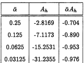
and are presented in Table 2.1. As a —> 0 it can be seen from these results th a t âA h —» —1, thus reinforcing the assumption (2.60) made in §2.4.3.
a ciAh
0.25 -2.8169 -0.704
0.125 -7.1173 -0.890
0.0625 -15.2531 -0.953 0.03125 -31.2355 -0.976
C H A P T E R 2. L IN E A R S T A B IL IT Y T H E O R Y 47
1.1
-y
1.0
-0.9
-
0.8-0.7
-0.6
-0.5
-0.4
-0.3
-0.2
-
0.1-0.0
-0 1 2 3 4
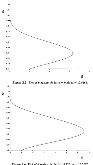
% Figure 2.3: Plot of y against for â = 0 .2 5 ; v q = 12.0 2 6 3 .
1.1
-V
1.0
-0.9
-0.8
-0.7
-0.6
-0.5
-0.4
-0.3
-0.1
-0.0
-2 3 4 5 6 7
0 1
C H A P T E R 2. L IN E A R S T A B IL IT Y T H E O R Y 48
1 .2 - 1
y
1.0-0.9
-0.8
-0.7
-0.6
-0.5
-0.4
-0.3
-0.2
-0.1
-0.0
-0 1 2 3 4 5 6 7 a 9 10 11 12 13 14 15 1
%
Figure 2.5: Plot of ÿ against 0o for a = 0.0625; vq = 24.4627.
1.1-V
1.0
-0.9
-0.8
-0.7
-0.6
-0.5
-0.4
-0.3
-0.1
-0.0
-2 10 12 16 18 20 22 24 26 28 30
0 4 6 8 14
%
C H A P T E R 2. L IN E A R S T A B IL IT Y T H E O R Y 49
/ |\
0(1)
\ l / \l/
0 1
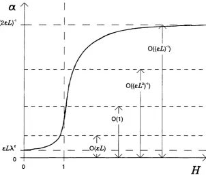
Figure 2.7: The variation of a as a function of the separation distance H.
2.6
A dditional com m ents and conclusion
In concluding this chapter we present graphically the variation of the wavenumber O' as a function of the scaled separation distance H . Figure 2,7 identifies th e regimes considered by indicating on the graph the size of a to leading order and maps the behaviour for a •< 1 as calculated numerically in §2.5.
We can see from the graph th a t as 5" oo the wavenumber approaches the value obtained when the presence of the wall is ignored, i.e. (2ei)~ ^. Moving our point of interest back upstream towards separation the effects of the wall become im portant. Here a = (ei))~^ao to leading order, where in term s of the separation distance H
a o = 1 — «0