areas: operational applications for coastal planning, decision
support and assessment
Achilleas G. Samaras1, Maria Gabriella Gaeta1, Adrià Moreno Miquel2, and Renata Archetti2
1CIRI – EC, Fluid Dynamics Unit, University of Bologna, Via del Lazzaretto 15/5, Bologna, 40131, Italy
2Department of Civil, Chemical, Environmental and Materials Engineering, University of Bologna, Viale Risorgimento 2,
Bologna, 40136, Italy
Correspondence to:Achilleas G. Samaras ([email protected])
Received: 24 February 2016 – Published in Nat. Hazards Earth Syst. Sci. Discuss.: 4 March 2016 Revised: 20 May 2016 – Accepted: 23 May 2016 – Published: 1 July 2016
Abstract. Numerical modelling has become an essential component of today’s coastal planning, decision support and risk assessment. High-resolution modelling offers an exten-sive range of capabilities regarding simulated conditions, works and practices and provides with a wide array of data regarding nearshore wave dynamics and hydrodynamics. In the present work, the open-source TELEMAC suite and the commercial software MIKE21 are applied to selected coastal areas of South Italy. Applications follow a scenario-based approach in order to study representative wave conditions in the coastal field; the models’ results are intercompared in order to test both their performance and capabilities and are further evaluated on the basis of their operational use for coastal planning and design. A multiparametric approach for the rapid assessment of wave conditions in coastal areas is also presented and implemented in areas of the same region. The overall approach is deemed to provide useful insights on the tested models and the use of numerical models – in gen-eral – in the above context, especially considering that the de-sign of harbours, coastal protection works and management practices in the coastal zone is based on scenario-based ap-proaches as well.
1 Introduction
Accurate predictions of waves, currents and sea level vari-ations in coastal areas are essential for a wide range of re-search and operational applications, as they govern
inunda-tion, sediment and pollutant transport, coastal morphology evolution and interactions with structures. Accordingly, nu-merical models that can serve the above purposes have be-come the main tool for researchers, engineers and policy-makers around the world involved in coastal planning, risk management and monitoring activities.
Following the above considerations, the development of reliable modelling systems or methods that can scale down from the ocean to the coastal scale has emerged as a need in today’s research. Reliable information on the hydrody-namics of the zone defined as nearshore, in particular, can serve a key role in coastal planning and hazard mitigation, as relevant processes at that scale differ significantly from those described in larger-scale oceanographic models. It is self-evident that, in the above context, the capabilities and limitations of such systems and methods – apart from their structure – would depend on those of the numerical models they comprise.
system (COAWST); Ge et al. (2013), who developed the FV-COM system to simulate multi-scale dynamics at the East China Sea shelf and the Changjiang Estuary; and Barnard et al. (2014), who developed a modelling system for predicting storm impact on high-energy coasts (CoSMoS).
In contrast, integrated systems comprising atmosphere, ocean and coastal models do present a number of chal-lenges for their users regarding both data interoperability and downscaling/nesting techniques, while they also demand significant computational expense in order to arrive to high-resolution simulations near coasts. Furthermore, for a series of activities in coastal/marine planning (e.g. identification of wave energy sites, see Reikard, 2009; Bozzi et al., 2014), vul-nerability/risk assessment (e.g. Stockdon et al., 2012; Idier et al., 2013; Archetti et al., 2016) and coastal protection mea-sures/infrastructure design (e.g. van Duin et al., 2004; Bur-charth et al., 2014; Karambas, 2014; Karambas and Samaras, 2014), either only parts of local hydrodynamics information are required (mainly wave properties to drive nearshore mod-els) or the respective approaches are based on the study of frequent/extreme condition scenarios. Accordingly, a num-ber of methods have been developed in order to estimate coastal wave properties from offshore information or larger-scale simulations. One can refer to the early work of O’Reilly and Guza (1993), who proposed wave energy transformation coefficients based on the comparison of two spectral wave models’ results or more recent ones using nesting and data assimilation schemes (Bertotti and Cavaleri, 2012; Rusu and Soares, 2014) and machine-learning techniques (Camus et al., 2011; Plant and Holland, 2011b, a). A work that stands out in recent literature is that of Long et al. (2014), who pro-posed a probabilistic method based on model scenarios for constructing wave time series at inshore locations.
The present work follows the rationale described above, comparing two modelling suites in the representation of nearshore dynamics and proposing a multiparametric scenario-based approach for the rapid assessment of wave conditions in coastal zones. Nevertheless, this work also served as the background study for the development of a modelling system coupling atmosphere, ocean and coastal dynamics, as described in Gaeta et al. (2016).
In the following, the open-source TELEMAC suite is compared with the well-known commercial software MIKE21 (developed by ©DHI Group) in fundamental wave/hydrodynamics modelling applications, aiming to test the models’ performance and the representation of the various processes governing wave propagation and wave-induced nearshore hydrodynamics. The latter (i.e. MIKE21) is also used for the implementation of the aforementioned multiparametric approach based on a trilinear interpolation algorithm. The study areas for the presented applications are all located in South Italy and comprise the coastal area around the city/port of Brindisi, the coastal area around the city/port of Bari and the Gulf of Taranto (the lat-ter only for the multiparametric approach’s applications).
TELEMAC and MIKE21 results are compared on the ba-sis of wave/current characteristics, along linear transects from the offshore to the nearshore and at specific points in-side/outside the breaker zone and near harbour entrances (for the study area of Bari). As for the scenario-based approach, its background and formulation are presented in detail, along with its implementation in the framework of an operational system, supporting the rationale behind this study and setting the basis for future work on the same path.
2 Methods
2.1 Wave and hydrodynamics modelling
Wave modelling within the TELEMAC and MIKE21 suites is performed using TOMAWAC and MIKE21-SW respec-tively. TOMAWAC and MIKE21-SW are characterized as third-generation spectral wave models, as they do not re-quire any parameterization on either the spectral or the direc-tional distribution of power (or action density). The physical processes modelled comprise (a) energy source/dissipation processes (wind-driven interactions with atmosphere, dissi-pation through wave breaking/whitecapping/wave-blocking due to strong opposing currents, bottom friction-induced dis-sipation); (b) non-linear energy transfer conservative pro-cesses (resonant quadruplet interactions, triad interactions); and (c) wave propagation-related processes (wave propaga-tion due to the wave group/current velocity, depth-/current-induced refraction, shoaling, interactions with unsteady cur-rents). The models compute the evolution of wave action densityN by solving the action balance equation (Booij et al., 1999):
∂N
∂t + ∇x, y
h
cg+UN i
+ ∂
∂σ(cσN )+ ∂
∂θ(cθN )= Stot
σ , (1)
whereN=E/σ, E being the variance density and σ the relative angular frequency,cgis the intrinsic group velocity
vector,U is the ambient current,cσ,cθ are the propagation velocities in spectral space (σ,θ) andStotis the source/sink
term that represents all physical processes which generate, dissipate or redistribute energy. Broken down to its compo-nents,Stotcan be written as
Stot=Sin+Swc+Snl4+Sbf+Sbr+Snl3, (2)
whereSinrepresents the energy transfer from wind to waves, Swc the dissipation of energy due to whitecapping,Snl4the
nonlinear transfer of energy due to quadruplet (four-wave) interactions, Sbf the dissipation due to bottom friction,Sbr
the dissipation due to wave breaking and Snl3 the
is also tested). As for diffraction, its effect is simulated using the phase-decoupled approach proposed by Holthui-jsen et al. (2003), based on the revised version of the Mild Slope Equation model of Berkhoff (1972) proposed by Porter (2003). Both models solve the governing equation by means of finite element-type methods to discretize geographical and spectral space, while the geographical domain is discretized by unstructured triangular meshes. Finally, and regarding specifically the coupling with 2-D hydrodynamics, it should be noted that the models compute and provide as output the four components of the radiation stress tensor,Sxx,Syy,Sxy andSyx, evaluated by
Sxx = Z Z E
2 h
2n(cosθ )2+(2n−1)idσdθ, (3)
Syy = Z Z E
2 h
2n(sinθ )2+(2n−1)idσdθ, (4)
Sxy =Syx= Z Z
Ensinθcosθdσdθ, (5)
as well as the respective wave-induced forces along thexand
yaxes (i.e.FxandFy), evaluated by integrating the radiation stresses over the water depth.
Hydrodynamics modelling within the TELEMAC and MIKE21 suites is performed using TELEMAC-2D and MIKE21-HD respectively. The models solve the 2-D shallow water equations (also referred to as Saint-Venant equations; see Hervouet, 2007), derived by integrating the Reynolds-averaged Navier–Stokes equations over the flow depth. Adopting the formulation of TELEMAC-2D for Cartesian coordinates, the equations of continuity and momentum along the x andy axes can be written as Eqs. (6), (7) and (8) respectively:
∂h
∂t +u·∇(h)+hdiv(u)=Sh, (6)
∂u
∂t +u·∇(u)= −g ∂ζ
∂x+Sx+
1
hdiv(hvt∇u) , (7)
∂v
∂t +u·∇(v)= −g ∂ζ
∂y+Sy+
1
hdiv(hvt∇v) , (8)
where h is the water depth, u, v are the velocity compo-nents anduthe velocity vector,gis the gravitational acceler-ation,vt is the momentum diffusion coefficient,ζ is the free surface elevation,Shis a term representing sources/sinks of
parameters. In the present work, the use of the hydrody-namics models is focused on the representation of wave-generated currents a task achieved through their direct cou-pling – through radiation stresses – with the respective spec-tral wave models within the TELEMAC and MIKE21 suites (see Eqs. (3)–(8) in the previous).
2.2 Multiparametric approach for the rapid assessment of nearshore wave conditions
The methodology followed in the present work for the rapid assessment of nearshore wave conditions (within the frame-work set in the previous; see Sect. 1) comprises a number of steps aiming to establish an efficient and computation-ally reasonable approach for operational use. The approach is scenario-based; thus its first step consists in defining a num-ber of scenarios representing wave conditions in the wider area of interest. This is done by performing a spectral anal-ysis of sea surface elevation records from nearshore/offshore buoys in order to produce a data set of three aggregated wave parameters, namely the significant wave heightHs, the peak
periodTpand the mean wave direction Dirm. Next, data set
parameters are further divided into a number of classes each, forming by aggregation the sets ofHs−Tp−Dirm,
hence-forth referred to as “scenarios”. These scenarios are after-wards used (in sequence) as boundary conditions for the wave model runs, resulting in an extensive data set of model results for the entire computational domain, stored in ASCII files that are properly named on the basis of the input wave scenarios. These files form the high-resolution wave con-ditions database along with a query algorithm, serving as the “bridge” between coarser-resolution operational models and the aforementioned produced data set. The query algo-rithm is responsible for (a) identifying the boundary wave conditions given by the coarser-resolution model (as sets of
Hs−Tp−Dirm) and (b) scanning the data set for the ASCII
file corresponding to the specific wave conditions and retriev-ing it. In the case that no data set file matches exactly the set of defined wave parameters, the algorithm will addition-ally (c) define the upper and lower classes’ boundaries for all three parameters (i.e.Hs,Tp, Dirm) on the basis of their
original query values, scan the data set and retrieve the re-spective ASCII files, (d) implement a trilinear interpolation in the three-dimensionalHs−Tp−Dirmspace (according to
computa-tional mesh and finally (e) store the derived parameter values in a new query-tailored ASCII file. The latter will represent the nearshore wave conditions for the query-defined set of wave parameters.
It should be noted that the division to a large number of pa-rameter classes at the first steps of this approach will lead to a large number of scenarios and, consequently, a large number of runs to be performed by the coastal wave model, with the respective effect on computational cost. However, this will accordingly lead to a higher accuracy of the trilinear inter-polation method as well, considering that its intrinsic error becomes lower with the increase in scenario discretization. Given that – in the framework of an operational system – response speed is of the essence, the combination of the spe-cific interpolation method with an adequately high number of defined scenarios is deemed to deliver the best performance overall due to its simplicity and implementation speed.
3 Application set-up 3.1 Model intercomparison 3.1.1 Conceptual approach
TELEMAC and MIKE21 have been extensively used over the years in research, operational and engineering design applications in maritime/coastal hydraulics; for MIKE21 this use leans significantly towards the last two cate-gories, it being one of the most widespread commercial suites for relevant applications. Their models have been separately evaluated and validated for several case stud-ies. Regarding TELEMAC, exemplary reference can be made to the work of Brière et al. (2007) on assessing its performance for a hydrodynamic case study; Brown and Davies (2009), Luo et al. (2013) and Villaret et al. (2013) on coupled wave/hydrodynamics–sediment trans-port/morphological modelling; Sauvaget et al. (2000) on the modelling of tidal currents; and Jia et al. (2015) on wave– current interactions in a river- and wave-dominant estuary. Regarding MIKE21, respective literature review would in-clude the work of Siegle et al. (2007) and Ranasinghe et al. (2010) on coupled wave/hydrodynamics–sediment trans-port/morphological modelling, Babu et al. (2005) on the modelling of tide-driven currents, Kong (2014) on the impact of tidal waves on storm surge and Aboobacker et al. (2009) and ArıGüner et al. (2013) on wave modelling. However, and given the fact that regarding system architecture and mod-elling components TELEMAC and MIKE21 have a lot of similarities (see also Sect. 2.1), literature has to show lim-ited references on their comparative evaluation.
The rationale behind the model intercomparison presented in the following derives from the general framework within which this work is carried out, that is the use of high-resolution wave and hydrodynamics models for (a) the
de-velopment and application of a multiparametric approach for the rapid assessment of wave conditions at inshore lo-cations (presented in Sects. 2.2 and 3.2) and (b) the develop-ment of a modelling system coupling atmosphere, ocean and coastal dynamics (presented in Gaeta et al., 2016). Accord-ingly, the TELEMAC and MIKE21 suites are compared in fundamental wave–hydrodynamics modelling applications, aiming to test models’ performance and the representation of the various processes governing wave propagation and wave-induced nearshore hydrodynamics. The comparison is per-formed for both single wave events and time series or random waves, representative of typical applications for coastal plan-ning, decision support and assessment. Apart from a coastal stretch near the city and harbour of Brindisi, applications (us-ing only TOMAWAC) are also performed for the area around the city of Bari, including its harbour. Specifically regarding the latter – and given the inherent limitations posed by the inclusion of diffraction in phase-averaged models – it should be noted that the objective was solely to test the extent to which spectral models like TOMAWAC could be used to cap-ture diffraction effects near harbour entrances (when the de-tailed agitation inside the harbour is not of interest), without the need to resort to separate time-demanding applications using phase-resolving models. The intercomparison also re-tains a strong user-oriented component, presenting examples of how models perform under typical coastal application sce-narios and how basic physical processes affect the computed parameters of interest.
3.1.2 Study areas and mesh generation
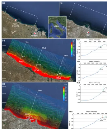
The first of the two study areas is located northwest of the city of Brindisi (South Italy), comprising Torre Guaceto, a marine protected area and state natural reserve of significant importance. The selected rectangular outline of the domain for the model applications measures about 21 km in the long-shore and 7.5 km in the cross-long-shore direction; Fig. 1a shows the wider study area and the aforementioned outline. The sec-ond study area comprises the coastal area around the city and harbour of Bari (South Italy); the outline of the com-putational domain in this case measures about 16.5 km in the longshore and 8.5 km in the cross-shore direction (see Fig. 1b).
As mentioned in Sect. 2.1, both the TELEMAC and MIKE21 modelling suites discretize the computational do-main by unstructured triangular meshes. Mesh generation for TELEMAC applications was done using Blue Kenue, a data preparation, analysis and visualization tool for hydraulic modellers developed by the National Research Council of Canada; the respective work for MIKE21 was done using MIKE Zero, the DHI tool for managing MIKE projects.
Figure 1.Satellite images of the wider areas, outlines of the computational domains, meshes, bathymetries, linear transects and points for results’ analysis for the Brindisi–Torre Guaceto(a, c)and Bari(b, d)case studies (background images from Google Earth, 2016; privately processed).
of Brindisi–Torre Guaceto the triangular mesh was created defining two density zones (20 m edge length below the −10 m isoline and 250 m for the rest of the field), resulting in a mesh consisting of 55 340 nodes forming 109 124 ele-ments. It should be noted that the mesh was first created in Blue Kenue and afterwards properly transformed to MIKE Zero format, maintaining the exact same nodes and connec-tions in order to exclude mesh-dependent divergences in the model runs. Figure 1c shows the mesh and bathymetry of the computational domain, along with the three linear tran-sects and six points for which model results will be intercom-pared (see Sect. 3.1.3). For the case study of Bari, three den-sity zones were defined arriving to the finest discretization of 10 m edge length in order to represent harbour structures, 250 m being the lowest discretization moving offshore. The
resulting mesh consists of 25 202 nodes forming 46 144 ele-ments; Fig. 1d shows the mesh and bathymetry of the com-putational domain, along with the linear transect and three points used for results’ analysis (see Sect. 3.1.3).
3.1.3 Application set-up for model intercomparison
Table 1.Overview of TELEMAC and MIKE21 model runs.
Run Forcing Processes Comparison along/at Compared parameters Figure(s)
Brindisi–T orre Guaceto Tc11 WE1 PRc1
TRc1, TRc2, TRc3 Hs,Tm, Dirmb 5, 6
Tc12 PRc2
Tc13 PRc3
Tc14a PRc4
Tc21
WE2
PRc1
TRc1, TRc2, TRc3 Hs,Tm, Dirm 7, 8
Tc22 PRc2
Tc23 PRc3
Tc24a PRc4
Tc31
TS1
PRc1
Tc32 PRc2 PTc1, PTc2, PTc3, Hs 9
Tc33 PRc3 PTc4, PTc5, PTc6 Curr. speed/directionc 10
Tc34a PRc4
Tc41
TS2
PRc1
Tc42 PRc2 PTc1, PTc2, PTc3, Hs 11
Tc43 PRc3 PTc4, PTc5, PTc6 Curr. speed/directionc 12
Tc44a PRc4
Bari
d
Th1
WE1 PRh1 TRh1 Hs,Tm, Dirm 13
Th1D PRh2
Th2
WE2 PRh1 TRh1 Hs,Tm, Dirm 13
Th2D PRh2
Th3
TS1 PRh1 PTh1, PTh2, PTh3 Hs,Tm, Dirm 14
Th3D PRh2
Th4
TS2 PRh1 PTh1, PTh2, PTh3 Hs,Tm, Dirm 14
Th4D PRh2
aTELEMAC-only run (see Sections 2.1 and 3.1.1). bH
sis significant wave height,Tmis mean wave period, Dirmis mean wave direction.
cCurrent speed/direction are intercompared only at PTc1, PTc2 and PTc3. dStand-alone TOMAWAC runs (see Sects. 2.1 and 3.1.1).
Bari case study refer to stand-alone TOMAWAC applica-tions, in the framework of the conceptual approach as pre-sented in Sect. 3.1.1. Every model run is assigned a different codename, henceforth used for its identification, with each line of Table 1 defining the forcing used (i.e. single wave events or time series of random waves); the processes in-cluded in the wave models’ set-up (see Table 2 and Sect. 2.1); the transects along which or the points at which results are intercompared; the parameters included in the comparison; and, finally, a reference to the figure(s) presenting the spe-cific results in Sect. 4.
The forcings were selected to represent a wide range of conditions regarding the wave climate in the areas of inter-est. The two single wave events selected, henceforth denoted as WE1 and WE2, represent the 50- and 2-year return period waves as resulted from the analysis of Regione Puglia (2009). The two 12 h time series selected, henceforth denoted as TS1 and TS2, were identified after analysis of wave data from the buoy of Monopoli (lat/long: 40◦58.50N, 17◦22.60E; depth: 90 m), part of the Italian wave metric network RON (“Rete
Table 2.Definition of the processes included in TELEMAC and MIKE21 spectral wave models’ set-up (see Table 1).
Processes Breaking Bottom Whitecapping Triads Triads
friction (LTA) (SPB)
Brindisi–Torre Guaceto
PRc1 √ √
PRc2 √ √ √
PRc3 √ √ √ √
PRc4a √ √ √ √
Barib
Processes Breaking Bottom Diffraction friction
PRh1 √ √
PRh2 √ √ √
aProcesses applied only to TELEMAC runs as Triads (SPB) are available only in TOMAWAC (see Sects. 2.1 and 3.1.1).
Figure 2.Characteristics of the wave events (WE1, WE2) and time series (TS1, TS2) used as forcings for TELEMAC and MIKE21 runs (see also Table 1).
Ondametrica Nazionale”; Corsini et al., 2006). All their char-acteristics are presented in Fig. 2.
The processes included in the wave models’ set-up are presented in Sect. 2.1. It should be highlighted that each of these common processes (also presented in Table 2) was in-cluded in the set-up of TOMAWAC and MIKE21-SW us-ing the same parameterizations. Energy transfer from wind to waves (term Sin in Eq. 2) and nonlinear energy
trans-fer due to quadruplet (four-wave) interactions (term Snl4in
Eq. 2) were not included, as their effects on spectral evolu-tion would have been insignificant for the model intercom-parison as it has been set-up on the basis of the rationale presented in Sect. 3.1.1 (i.e. focus on the nearshore, dictat-ing the relatively small size of the computational domain in the cross-shore direction).
Considering that model results presented over the entire computational domain (as 2-D fields of the respective param-eters) would pose significant challenges to the perceptibility of any intercomparison attempt (between both different mod-elling suites and different processes), it was deemed prefer-able to compare model results along linear transects from the offshore computational boundary to the shoreline (for WE1 and WE2) or at specific points (for TS1 and TS2). For the Brindisi–Torre Guaceto case study, transects TRc1, TRc2 and TRc3 were defined in order to capture areas of differ-ent/representative bathymetry profiles alongshore; the pairs of points PTc1–PTc4, PTc2–PTc5 and PTc3–PTc6 were de-fined at specific locations of the aforementioned transects re-spectively. The first point of each of the previous pairs was selected to fall within the breaker zone and second one before the breaker line; given that – regarding the hydrodynamics – the objective was to compare wave-generated currents, the hydrodynamics models’ results were analysed only at points PTc1, PTc2 and PTc3. The locations of the points were de-cided to not change between runs for different forcings, in order to facilitate the comprehensibility of the presented re-sults. For the Bari case study, the objective being to test the diffraction algorithm’s performance in spectral wave models (see also Sect. 3.1.1), one transect was defined (TRh1) and three points along it: one at the vicinity of the outer
break-water tip (PTh1), one right at the middle of the harbour’s entrance (PTh2) and one inside the harbour close to the en-trance (PTh3). All transects, points and bathymetric profiles are presented in Fig. 1c and d.
3.2 Multiparametric approach for the rapid assessment of wave conditions
The multiparametric approach presented in this work was ap-plied to three areas of interest in South Italy: the areas around the cities/ports of Brindisi and Bari, as well as the Gulf of Taranto (see Fig. 3). Accordingly, the scenarios represent-ing wave conditions in the wider area were defined based on the analysis of data from the buoys of Monopoli (lat/long: 40◦58.50N, 17◦22.60E; depth: 90 m; see Fig. 3) and Crotone (lat/long: 39◦01.40N, 17◦13.20E; depth: 95 m; see Fig. 3), covering the period from 1 January 1989 to 31 December 2012. For each buoy data set, wave parameters were further divided into a number of classes each – according to Table 3 – forming by aggregation the scenarios to be used for the wave model runs (i.e. sets ofHs−Tp−Dirm). Figure 4a and b
show the frequencies of occurrence of the scenarios’Hs−Tp
andHs−Dirmpairs respectively for the Monopoli data set;
Fig. 4c and d show the respective frequencies for Crotone. It should be noted that all directions follow the nautical di-rection convention; negative values were used in Fig. 4b for representation issues, as gaps in certain direction ranges (i.e. corresponding to what would be seaward wave origins) were omitted.
Figure 3. Computational domain outlines for the three areas in South Italy where the proposed multiparametric approach was ap-plied and locations of the Monopoli and Crotone buoys; the grid lines and points represent the WAVEWATCH III rectilinear grid (background image from Google Earth (2016); privately processed).
Table 3.Class properties applied to the wave parameter data sets for scenarios’ definition.
Parameter Minimum Maximum Class step
Hs(m) 0.1 6 0.1
Tp(s) 1.5 12 0.5
Dirm(◦) 0 355 5
results created three extensive data sets (one for each study area), stored in properly named ASCII files, as described in Sect. 2.2. The performance of the developed query algorithm, also described in Sect. 2.2, was tested for a series of exem-plary cases before its operational implementation.
In the framework of the Research Project “TESSA” (De-velopment of Technologies for the Situational Sea Aware-ness), the specific multiparametric approach was applied using WAVEWATCH III (Tolman, 2009) as the coarser-resolution model that would feed sets ofHs−Tp−Dirmto
the query algorithm in order to retrieve/create the nearshore wave conditions file (based on MIKE-SW results); the model’s rectilinear grid is presented in Fig. 3.
Figure 4.Frequencies of occurrence of the scenarios’Hs−Tpand Hs−Dirmpairs for the Monopoli data set (aandbrespectively) and
the Crotone data set (canddrespectively).
4 Results and discussion
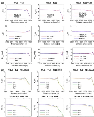
As described in Sect. 3.1 and presented in Tables 1 and 2, model intercomparison regards the Brindisi–Torre Guaceto case study. Figures 5 and 6 show the comparison of TELEMAC and MIKE21 results (Hs−Tm−Dirm) along
tran-sects TRc1, TRc2 and TRc3 for forcing WE1, as well as the effect of different processes onHs along the specific
tran-sects, separately for each modelling suite; Figs. 7 and 8 show the respective results for forcing WE2. The overall agree-ment between model results is good, and all parameters are very close for the majority of runs for both forcings, with a general observation being that TELEMAC constantly pro-duces slightly higher values ofHs and lower values ofTm
than MIKE21. The extensive set of runs tested allows for a more detailed analysis of the models’ performance, as pre-sented in the following. For runs Tc11 and Tc21, including the processes of breaking and bottom friction dissipation,Hs
values are practically overlapping along most part of all three transects, with the exception of the divergences observed at the vicinity of the breaker line (more noticeable for the rela-tively mild slope TRc1 rather than TRc2 and TRc3);Tmand
Dirmshow small divergences as well, mostly noticeable after
breaking for the steeper slope profiles of TRc2 and TRc3 and for the higher-wave forcing WE1 (i.e. Tc11 run). The inclu-sion of the process of energy dissipation due to whitecapping in runs Tc12 and Tc22 results in a small decrease ofHs
over-all, which is more clearly noticeable in Figs. 6b and 8b pre-senting such effects separately for TELEMAC and MIKE21; changes inTmand Dirmare barely noticeable between Tc11–
Figure 5.Comparison of TELEMAC and MIKE21 results (Hs−Tm−Dirm) along transects(a)TRc1 and(b)TRc2, for the Brindisi–Torre
Guaceto case study (forcing WE1;∗=Tc14).
to the shallow water sections of the studied profiles/transects where the specific process’s effect becomes significant. Al-though both suites use the LTA model of Eldeberky and Bat-tjes (1983), the inclusion of triads seems to have a rather small effect on MIKE21Hs results (slight decrease of wave
height and shift of the breaker line seaward), with the ef-fect on the wave energy spectrum, however, becoming more
evident when comparingTmvalues. In contrast, TELEMAC
runs result in higher Hs values right before breaking and
quite lowerTmvalues inshore. Dirmresults show small
Figure 6. (a)Comparison of TELEMAC and MIKE21 results (Hs−Tm−Dirm) along transect TRc3 for the Brindisi–Torre Guaceto case
study (forcing WE1;∗=Tc14);(b)effect of different processes onHsfor TELEMAC (top) and MIKE21 (bottom).
Tc14 in the set of runs, and its results are represented as dot-ted lines in all figures (nodot-ted accordingly). Following Becq-Girard et al. (1999) remarks on the validity range of the LTA model, Tc14 results show indeed a quite different represen-tation of the process by TOMAWAC, with milder evolution of the wave energy onshore and smaller changes to all pa-rameter values than Tc13 produced (see Figs. 6b and 8b in particular).
Figures 9 and 10 show the comparison of TELEMAC and MIKE21 results (Hsand Curr. speed/direction respectively),
for the time series forcing TS1; Figs. 11 and 12 show the
respective results for forcing TS2. Significant wave height values are compared at points along transects TRc1, TRc2 and TRc3 (see Fig. 1), three of them within the breaker zone (PTc1, PTc2, PTc3) and three outside of it (PTc4, PTc5, PTc6); the wave-generated currents’ speed and direc-tion are compared only at points PTc1, PTc2 and PTc3 (see also Sect. 3.1.3). RegardingHs, the comparison between
insignif-Figure 7.Comparison of TELEMAC and MIKE21 results (Hs−Tm−Dirm) along transects(a)TRc1 and(b)TRc2, for the Brindisi–Torre
Guaceto case study (forcing WE2;∗=Tc24).
icant) for various operational, planning and engineering de-sign applications in coastal areas. TELEMAC and MIKE21 results at points PTc4, PTc5 and PTc6 are close and in-phase for all processes, with higher discrepancies observed for the higher-wave forcing TS2. At points PTc1, PTc2 and PTc3, the conclusions drawn from the analysis of the wave events’ results in the previous can be clearly identified here
as well, with the most significant alterations in the differ-ent suites’ results observed again for the runs where triad interactions were included in the modelled processes (i.e. Tc33/Tc34 and Tc43/Tc44); it should be also noted that the higher-wave forcing TS2 leads to smaller variations ofHs
Regard-Figure 8. (a)Comparison of TELEMAC and MIKE21 results (Hs−Tm−Dirm) along transect TRc3 for the Brindisi–Torre Guaceto case
study (forcing WE2;∗=Tc24);(b)effect of different processes onHsfor TELEMAC (top) and MIKE21 (bottom).
ing the wave-generated currents, TELEMAC and MIKE21 results are in relatively good agreement for all runs consider-ing the order of magnitude of the resultconsider-ing current speeds, as well as the sensitivity of current directions within the break-ing zone. Figure 10 shows that for runs Tc31 and Tc32 results are very close with the exception of the period up to hour 4 at PTc1, where TELEMAC shows current speeds close to zero (with the respective effect on current direction). As noted in the previous, the introduction of triad interactions results in a more significant effect when modelled with TELEMAC, al-though the SPB model does lead to smoother results
regard-ing both speed and direction (run Tc34). Point PTc3 shows larger divergences than points PTc1 and PTc2 that attributed to the combination of its location in the computational do-main and the significant shift in the forcing’s direction after hour 6 (see Fig. 2). Figure 12 shows that at points PTc1 and PTc2 results are in good agreement for both TELEMAC and MIKE21, following the remark regarding the smallHs
Figure 9.Comparison of TELEMAC and MIKE21 results (Hs) at points within (PTc1, PTc2, PTc3) and outside of the breaker zone (PTc4,
PTc5, PTc6) for the Brindisi–Torre Guaceto case study for runs(a)Tc31,(b)Tc32 and(c)Tc33/Tc34∗.
Regarding the Bari case study, it should be stated again (as in Sect. 3.1.1) that the objective of its inclusion in this work was solely to test the extent to which spectral mod-els could be used to capture diffraction effects near harbour entrances in the framework of operational approaches like the one presented in Sect. 3.2. This was done while keep-ing in mind the inherent limitations posed by the inclusion of
dif-Figure 10.Comparison of TELEMAC and MIKE21 results (Curr. speed/direction) at points within the breaker zone (PTc1, PTc2, PTc3) for the Brindisi–Torre Guaceto case study for runs(a)Tc31,(b)Tc32 and(c)Tc33/Tc34∗.
ferences in wave characteristics around the breakwater’s tip and near the harbour entrance, while the model also man-ages to capture the diffusion of the wave height inside the harbour area; larger effects are observed for the higher-wave forcing WE1. Figure 14 shows TOMAWAC results (with and without the inclusion of diffraction) at points PTh1, PTh2 and PTh3 for forcings TS1 and TS2 (Fig. 14a and b
respec-tively). Differences are noticeable for all parameters, being relatively more significant at points PTh2–PTh3 and for the higher-wave forcing TS2.
Figure 11.Comparison of TELEMAC and MIKE21 results (Hs) at points within (PTc1, PTc2, PTc3) and outside of the breaker zone (PTc4,
PTc5, PTc6) for the Brindisi–Torre Guaceto case study for runs(a)Tc41,(b)Tc42 and(c)Tc43/Tc44∗.
characteristics to the query algorithm in order to provide nearshore wave conditions from the created database of MIKE-SW results. Its performance was tested for a series of different wave conditions for the three areas of interest (i.e. Brindisi, Bari and Gulf of Taranto; see Fig. 3) and the algo-rithm managed to deliver results in a fast and seamless way at all times.
5 Conclusions
Figure 12.Comparison of TELEMAC and MIKE21 results (Curr. speed/direction) at points within the breaker zone (PTc1, PTc2, PTc3) for the Brindisi–Torre Guaceto case study for runs(a)Tc41,(b)Tc42 and(c)Tc43/Tc44∗.
zones that aims to serve as an operational tool for coastal planning, decision support and assessment. The study areas for the presented applications are all located in South Italy and comprise the coastal area around the city/port of Brindisi, the coastal area around the city/port of Bari and the Gulf of Taranto. For the first one, TELEMAC and MIKE21 are inter-compared for a series of application set-ups aiming to test the
Figure 13.Comparison of TOMAWAC results for the Bari case study:(a, d)along transect TRh1 for forcings WE1 and WE2 respectively;
(b, c)and(e, f)as wave fields at the harbour of Bari for forcings WE1 and WE2 respectively.
diffraction effects near harbour entrances, in the framework of operational approaches like the one presented in this work when the detailed agitation inside the harbour is not of in-terest. TELEMAC and MIKE21 results are compared on the basis of wave/current characteristics, along linear transects from the offshore to the nearshore and at specific points in-side/outside the breaker zone and near the entrance of the harbour for the study area of Bari. Analysis shows an over-all satisfactory agreement between the two modelling suites and is deemed to provide useful insights on both their
Figure 14.Comparison of TOMAWAC results (Hs−Tm−Dirm) for the Bari case study at points PTh1, PTh2 and PTh3 for forcings(a)TS1
and(b)TS2.
of wave scenarios on the basis of field measurements, a data set of wave model results using these scenarios as boundary conditions and a query algorithm based on the trilinear inter-polation that bridges coarser-resolution operational models and the aforementioned data set in order to provide query-tailored fields of nearshore wave dynamics. The implemen-tation of the specific approach as part of an operational chain
thank the Handling Editor Ivan Federico and the two referees for their constructive comments and suggestions.
Edited by: I. Federico
Reviewed by: C. Koutitas and one anonymous referee
References
Aboobacker, V. M., Vethamony, P., Sudheesh, K., and Rupali, S. P.: Spectral characteristics of the nearshore waves off Paradip, India during monsoon and extreme events, Nat. Hazards, 49, 311-323, doi:10.1007/s11069-008-9293-8, 2009.
Archetti, R., Paci, A., Carniel, S., and Bonaldo, D.: Optimal in-dex related to the shoreline dynamics during a storm: the case of Jesolo beach, Nat. Hazards Earth Syst. Sci., 16, 1107–1122, doi:10.5194/nhess-16-1107-2016, 2016.
ArıGüner, H. A., Yüksel, Y., and Özkan Çevik, E.: Estimation of wave parameters based on nearshore wind–wave correlations, Ocean Eng., 63, 52–62, doi:10.1016/j.oceaneng.2013.01.023, 2013.
Babu, M. T., Vethamony, P., and Desa, E.: Modelling tide-driven currents and residual eddies in the Gulf of Kachchh and their seasonal variability: A marine environmen-tal planning perspective, Ecol. Model., 184, 299–312, doi:10.1016/j.ecolmodel.2004.10.013, 2005.
Barnard, P., van Ormondt, M., Erikson, L., Eshleman, J., Hapke, C., Ruggiero, P., Adams, P., and Foxgrover, A.: Development of the Coastal Storm Modeling System (CoSMoS) for predicting the impact of storms on high-energy, active-margin coasts, Nat. Hazards, 74, 1095–1125, doi:10.1007/s11069-014-1236-y, 2014. Battjes, J. A. and Janssen, J. P. F. M.: Energy loss and set-up due to breaking of random waves, 16th International Conference on Coastal Engineering, 27 August–3 September 1978, Hamburg, Germany, 569–587, 1978.
Becq-Girard, F., Forget, P., and Benoit, M.: Non-linear propaga-tion of unidirecpropaga-tional wave fields over varying topography, Coast. Eng., 38, 91–113, doi:10.1016/S0378-3839(99)00043-5, 1999. Becq, F.: Extension de la modélisation spectrale des états de mer
vers le domaine côtier, PhD thesis, Université de Toulon et du Var, La Garde, France, 251 pp., 1998.
Berkhoff, J. C. W.: Computation of combined refraction - diffrac-tion, 13th International Conference on Coastal Engineering, 10– 14 July 1972, Vancouver, Canada, 471–490, 1972.
Bertotti, L. and Cavaleri, L.: Modelling waves at Orkney coastal locations, J. Marine Syst., 96–97, 116–121, doi:10.1016/j.jmarsys.2012.02.012, 2012.
ment of TELEMAC system performances, a hydrodynamic case study of Anglet, France, Coast. Eng., 54, 345-356, doi:10.1016/j.coastaleng.2006.10.006, 2007.
Brown, J. M. and Davies, A. G.: Methods for medium-term pre-diction of the net sediment transport by waves and currents in complex coastal regions, Cont. Shelf Res., 29, 1502–1514, doi:10.1016/j.csr.2009.03.018, 2009.
Burcharth, H. F., Lykke Andersen, T., and Lara, J. L.: Upgrade of coastal defence structures against increased loadings caused by climate change: A first methodological approach, Coast. Eng., 87, 112–121, doi:10.1016/j.coastaleng.2013.12.006, 2014. Camus, P., Mendez, F. J., Medina, R., and Cofiño, A. S.:
Analysis of clustering and selection algorithms for the study of multivariate wave climate, Coast. Eng., 58, 453-462, doi:10.1016/j.coastaleng.2011.02.003, 2011.
Corsini, S., Inghilesi, R., Franco, L., and Piscopia, R.: Italian Waves Atlas, APAT-Università degli Studi di Roma 3, Rome, Italy, 134 pp., 2006.
Eldeberky, Y. and Battjes, J. A.: Parameterisation of triads interac-tions in wave energy models, Coastal Dynamics Conference ’95, 4–8 September 1995, Gdansk, Poland, 140–148, 1983.
Gaeta, M. G., Samaras, A. G., Federico, I., and Archetti, R.: A cou-pled wave-3D hydrodynamics model of the Taranto Sea (Italy): a multiple-nesting approach, Nat. Hazards Earth Syst. Sci. Dis-cuss., doi:10.5194/nhess-2016-95, in review, 2016.
Ge, J., Ding, P., Chen, C., Hu, S., Fu, G., and Wu, L.: An integrated East China Sea-Changjiang Estuary model system with aim at resolving multi-scale regional-shelf-estuarine dynamics, Ocean Dynam., 63, 881–900, doi:10.1007/s10236-013-0631-3, 2013. Google Earth: Image©2016 TerraMetrics, Data SIO, NOAA, U.S.
Navy, NGA, GEBCO, 2016.
Hasselmann, K., Barnett, T. P., Bouws, E., Carlson, H., Cartwright, D. E., Enke, K., Ewing, J. A., Gienapp, H., Hasselmann, D. E., Kruseman, P., Meerburg, A., Müller, P., Olbers, D. J., Richter, K., Sell, W., and Walden, H.: Measurements of wind-wave growth and swell decay during the Joint North Sea Wave Project (JONSWAP), Deutsches Hydrographisches Institut, Hamburg, Ergänzungsheft zur Deutschen Hydrographischen Zeitschrift, Reihe A (8◦), Nr. 12, 95 pp., 1973.
Hervouet, J.-M.: Hydrodynamics of Free Surface Flows: Modelling with the finite element method, John Wiley & Sons Ltd, New Jersey, USA, 360 pp., 2007.
Holthuijsen, L. H., Herman, A., and Booij, N.: Phase-decoupled refraction–diffraction for spectral wave models, Coast. Eng., 49, 291–305, doi:10.1016/S0378-3839(03)00065-6, 2003.
Earth Syst. Sci., 13, 999–1013, doi:10.5194/nhess-13-999-2013, 2013.
Janssen, P. A. E. M.: Quasi-linear Theory of
Wind-Wave Generation Applied to Wave Forecasting,
J. Phys. Oceanogr., 21, 1631–1642, doi:10.1175/1520-0485(1991)021<1631:qltoww>2.0.co;2, 1991.
Jia, L., Wen, Y., Pan, S., Liu, J. T., and He, J.: Wave–current inter-action in a river and wave dominant estuary: A seasonal contrast, Appl. Ocean Res., 52, 151–166, doi:10.1016/j.apor.2015.06.004, 2015.
Karambas, T. V.: Modelling of climate change impacts on coastal flooding/erosion, ports and coastal defence structures, Desalination and Water Treatment, 54, 1–8, doi:10.1080/19443994.2014.934115, 2014.
Karambas, T. V. and Samaras, A. G.: Soft shore protection methods: The use of advanced numerical models in the evaluation of beach nourishment, Ocean Eng., 92, 129–136, doi:10.1016/j.oceaneng.2014.09.043, 2014.
Komen, G. J., Hasselmann, K., and Hasselmann, K.: On the Existence of a Fully Developed Wind-Sea Spectrum, Journal of Physical Oceanography, 14, 1271–1285, doi:10.1175/1520-0485(1984)014<1271:oteoaf>2.0.co;2, 1984.
Kong, X.: A numerical study on the impact of tidal waves on the storm surge in the north of Liaodong Bay, Acta Oceanol. Sin., 33, 35–41, doi:10.1007/s13131-014-0430-9, 2014.
Kreyszig, E.: Advanced Engineering Mathematics, John Wiley & Sons, Inc., New Jersey, USA, 2010.
Long, J. W., Plant, N. G., Dalyander, P. S., and Thompson, D. M.: A probabilistic method for constructing wave time-series at in-shore locations using model scenarios, Coast. Eng., 89, 53–62, doi:10.1016/j.coastaleng.2014.03.008, 2014.
Luo, J., Li, M., Sun, Z., and O’Connor, B. A.: Numerical modelling of hydrodynamics and sand transport in the tide-dominated coastal-to-estuarine region, Mar. Geol., 342, 14–27, doi:10.1016/j.margeo.2013.06.004, 2013.
O’Reilly, W. C. and Guza, R. T.: A comparison of two spectral wave models in the Southern California Bight, Coast. Eng., 19, 263– 282, doi:10.1016/0378-3839(93)90032-4, 1993.
Ozer, J., Padilla-Hernández, R., Monbaliu, J., Alvarez Fanjul, E., Carretero Albiach, J. C., Osuna, P., Yu, J. C. S., and Wolf, J.: A coupling module for tides, surges and waves, Coast. Eng., 41, 95–124, doi:10.1016/S0378-3839(00)00028-4, 2000.
Plant, N. G. and Holland, K. T.: Prediction and assim-ilation of surf-zone processes using a Bayesian net-work: Part II: Inverse models, Coast. Eng., 58, 256–266, doi:10.1016/j.coastaleng.2010.11.002, 2011a.
Plant, N. G. and Holland, K. T.: Prediction and assim-ilation of surf-zone processes using a Bayesian net-work: Part I: Forward models, Coast. Eng., 58, 119–130, doi:10.1016/j.coastaleng.2010.09.003, 2011b.
Porter, D.: The mild-slope equations, J. Fluid Mech., 494, 51–63, 2003.
Ranasinghe, R., Larson, M., and Savioli, J.: Shoreline response to a single shore-parallel submerged breakwater, Coast. Eng., 57, 1006–1017, doi:10.1016/j.coastaleng.2010.06.002, 2010. Regione Puglia: Il clima meteomarino sul litorale pugliese, Regione
Puglia – Assessorato Trasparenza e Cittadinanza Attiva, 355 pp., 2009.
Reikard, G.: Forecasting ocean wave energy: Tests
of time-series models, Ocean Eng., 36, 348–356,
doi:10.1016/j.oceaneng.2009.01.003, 2009.
Rusu, L. and Soares, C. G.: Local data assimilation scheme for wave predictions close to the Portuguese ports, Journal of Operational Oceanography, 7, 45–57, 2014.
Sauvaget, P., David, E., and Guedes Soares, C.: Modelling tidal currents on the coast of Portugal, Coast. Eng., 40, 393–409, doi:10.1016/s0378-3839(00)00020-x, 2000.
Siegle, E., Huntley, D. A., and Davidson, M. A.: Coupling video imaging and numerical modelling for the study of inlet morpho-dynamics, Mar. Geol., 236, 143–163, 2007.
Stockdon, H. F., Doran, K. J., Thompson, D. M., Sopkin, K. L., Plant, N. G., and Sallenger, A. H.: National assessment of hurricane-induced coastal erosion hazards-Gulf of Mexico, U.S. Geological Survey, Open-File Report 2012–1084, 51 pp., 2012. Tolman, H. L.: User manual and system documentation of
WAVE-WATCH III version 3.14, NOAA/NWS/NCEP/MMAB, 194 pp., 2009.
van Duin, M. J. P., Wiersma, N. R., Walstra, D. J. R., van Rijn, L. C., and Stive, M. J. F.: Nourishing the shoreface: observations and hindcasting of the Egmond case, The Netherlands, Coast. Eng., 51, 813–837, doi:10.1016/j.coastaleng.2004.07.011, 2004. Villaret, C., Hervouet, J. M., Kopmann, R., Merkel, U.,
and Davies, A. G.: Morphodynamic modeling using the Telemac finite-element system, Comput. Geosci., 53, 105–113, doi:10.1016/j.cageo.2011.10.004, 2013.