The computation of blood flow waveforms from digital X-ray angiographic data

(1)

2 8 0 7 7 1 3 6 7 2

THE COMPUTATION OF BLOOD FLOW WAVEFORMS FROM DIGITAL

X-RAY ANGIOGRAPHIC DATA

by

Alexander M Seifalian

M.Sc., PGDip.Com., OPhys., MlnstP., MIPSM.

Thesis submitted for the Degree of Doctor of Philosophy for the University of London

. :..U;CAL LIUKARY. <OYAL HOSriTA

l-lAMPSTEAiX June 1993

University Department of Surgery Royal Free Hospital School of Medicine London NWS 2QG, UK.

(2)

ProQuest Number: U057118

INFORMATION TO ALL USERS

The quality of this reproduction is dependent upon the quality of the copy submitted.

In the unlikely event that the author did not send a complete manuscript and there are missing pages, these will be noted. Also, if material had to be removed,

a note will indicate the deletion.

uest.

ProQuest U057118

Published by ProQuest LLC(2016). Copyright of the Dissertation is held by the Author.

This work is protected against unauthorized copying under Title 17, United States Code. Microform Edition © ProQuest LLC.

ProQuest LLC

789 East Eisenhower Parkway P.O. Box 1346

(3)

(4)

ABSTRACT

This thesis investigates a novel technique for the quantitative measurement of

pulsatile blood flow waveforms and mean blood flow rates using digital X-ray

angiographic data.

Blood flow waveforms were determined following an intra-arterial injection of

contrast material. Instantaneous blood velocities were estimated by generating

a ‘parametric image’ from dynamic X-ray angiographic images in which the image

grey-level represented contrast material concentration as a function of time and

true distance in three dimensions along a vessel segment.

Adjacent concentration-distance profiles in the parametric image of iodine

concentration versus distance and time were shifted along the vessel axis until

a match occurred. A match was defined as the point where the mean sum of the

squares of the differences between the two profiles was a minimum. The distance

translated per frame interval gave the instantaneous contrast material bolus

velocity.

The technique initially was validated using synthetic data from a computer

simulation of angiographic data which included the effect of pulsatile blood flow

and X-ray quantum noise. The data were generated for a range of vessels from

2 mm to 6 mm in diameter. Different injection techniques and their effects on the

accuracy of blood flow measurements were studied.

Validation of the technique was performed using an experimental phantom of

blood circulation, consisting of a pump, flexible plastic tubing, the tubular probe

of an electromagnetic flowmeter and a solenoid to simulate a pulsatile flow

waveform which included reverse flow.

The technique was validated for both two- and three-dimensional representations

of the blood vessel, for various flow rates and calibre sizes. The effects of various

physical factors were studied, including the distance between injection and

(5)

Finally, this method was applied to clinical data from femoral arteries and arteries

in the head and neck.

(6)

-3-CONTENTS

Page

Title page 1

Abstract 2

Contents 4

Figures 9

Tables 16

Acknowledgments 18

Chapter 1 Introduction 20

1.1 Introduction 20

1.2 Application of blood flow measurements 21

1.2.1 Arterial flow velocity waveform patterns 22

1.3 Structure of Thesis 23

Chapter 2 A review of existing methods of measuring flow In blood

vessels 25

2.1 Introduction 25

2.2 Methods 26

2.2.1 The electromagnetic flowmeter 26

2.2.2 The thermodilution technique 26

2.2.3 Doppler ultrasound 27

2.2.4 Nuclear magnetic resonance 32

2.3 Conclusion 33

Chapter 3 Physics and Instrumentation of digital angiography 34

3.1 Introduction 34

3.2 Principles of digital fluorographic imaging 34

3.2.1 X-ray tube and generator 36

(7)

3.2.3 Video camera 38

3.2.4 Analogue-to-digital conversion 39

3.2.5 Image analysis workstations 40

3.3 Digital subtraction angiography 40

3.4 Error in formation of digital images 43

3.4.1 Noise 43

3.4.2 Scatter and veiling glare 45

3.5 Conclusion 45

Chapter 4 A review of quantitative X-ray angiographic techniques to

measure biood fiow and vessei caiibre 47

4.1 Introduction 47

4.2 Methods of measuring blood flow 48

4.2.1 Dye-dilution technique 48

4.2.1.1 Bolus injection 49

4.2.1.2 Constant rate injection 51

4.2.2 Bolus transport time technique 52

4.2.2.1 Bolus transport time estimation using part

of the time-density curves 54

4.2.2.2 Bolus transport time estimation using whole

of the time-density curves 54

4.2.2.3 Measurement of the leading edge of the bolus 56

4.2.3 Distance-density Curves 60

4.2.3.1 Distance between rapidly pulsed boluses 60

4.2.3.2 Tracking of bolus mass 61

4.2.3.3 Calculation of velocity using a grey-level

gradient operator 62

4.3 Methods to measure vessel cross-sectional area 64

4.3.1 Geometric approaches 65

4.3.2 Densitometric approaches 68

4.4 Discussion 71

(8)

-5-Chapter 5 Three dimensional reconstruction of vascular structures 75

5.1 Introduction 75

5.2 Method 78

5.2.1 The transformation matrix 79

5.2.2 Determination of the transformation matrix 80

5.2.3 Reconstruction of 3D skeleton 82

5.3 Implementation of the technique 82

5.4 Radiography 82

5.5 3D reconstruction of the arterial tree using a system for

angiographic reconstruction and analysis (SARA) 83

5.5.1 Identification of corresponding points between two

projection views 85

5.5.2 Blood vessel centre line definition 88

5.5.3 Calculation of the edges of a blood vessel 89

5.6 Cross-sectional area estimation 91

5.7 Validation of SARA 91

5.7.1 Method and materials 94

5.7.2 Analysis 94

5.7.3 Results 97

5.8 Discussion and conclusion 97

Chapter 6 A new method for deriving pulsatile biood flow waveforms 101

6.1 Introduction 101

6.2 Theory 101

6.2.1 Concept of parametric images 101

6.2.2 Extraction of blood velocity waveform from

parametric images 103

6.3 Method 111

6.3.1 Principle of the technique 111

6.3.2 Generation of parametric images 112

6.3.3 Calculation of instantaneous blood velocities 113

6.3.4 Implementation of the technique and testing 113

6.3.5 Tuning the velocity algorithm 113

6.3.6 Computation of volume blood flow waveforms and

(9)

6.4 Discussion 115

Chapter 7 Assessment of blood flow measurement techniques using

synthetic data from computer simulated model 116

7.2 Methods and materials 117

7.2.1 Description of the numerical model 117

7.2.1.1 Accuracy of modelling techniques 118

7.2.2 Description of the validation experiment 120

7.2.2.1 Input parameters to the model 120

7.2.2 2 Injection strategy for contrast material 120

7.2 2.3 Generation of dynamic angiographic data using

the computer model 124

7.2.2.4 Generation of data 126

7.2.3 Blood flow measurement algorithms 129

7.2.3.1 Bolus transport time 129

7.2.3.2 Tracking of bolus mass 130

7.2 3.3 Matching distance-density curves over time 130

7.3 Results 130

7.3.1 Transport time calculated from two time-density curves 130

7.3.2 Bolus mass tracking and distance-density curve

matching 132

7.4 Discussion 138

Chapter 8 Validation of flow studies in physical models 143

8.2 Method and materials 143

8.2.1 Construction of phantom 143

8.2.2 Electromagnetic flowmeter 148

8.2.3 Radiography 148

8.2.4 Image analysis 149

8.2.5 Statistical methods 150

8.3 Results 150

8.3.1 Electromagnetic flowmeter 150

8.3.2 2D data processing 152

(10)

-7-8.3.3 3D data processing 160

8.4 Discussion and conclusion 164

Chapter 9 Application to clinical data 174

9.2 Method and materials 175

9.2.1 Radiography 175

9.2.2 Femoral artery 175

9.2.3 Head and neck 176

9.3 Results 181

9.3.1 Femoral artery 181

9.3.2 Head and neck 181

9.4 Discussion 190

9.4.2 Femoral artery study 190

9.4.3 Vessels in the head and neck 192

Chapter 10 Summary and conclusions 194

10.2 Advantages of our angiographic flow technique 196

10.3 Limitations of our angiographic flow technique 197

10.4 Future directions 199

Appendix Theory of absolute cross-sectional area 202

References 204

(11)

FIGURES

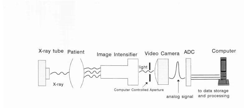
Fig. 3.1. Block diagram of basic system used for digital fluorography. The main imaging components include: X-ray tube, image intensifier,

video camera, high speed analogue-to-digital converter (ADC), and

a computer.

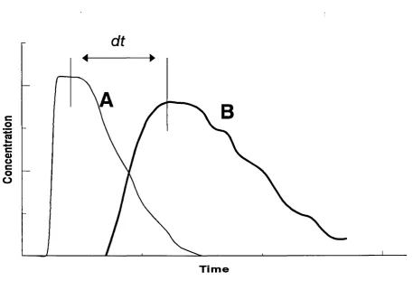
Fig. 4.1. Schematic illustration of the basis for calculation of blood flow from the transport time. The time df for passage of a contrast bolus from

a ROI (A) to a ROI (B) is measured. The average velocity V and

flow can be calculated from the distance dS between the ROIs and

the diameter (O) of the blood vessel segment.

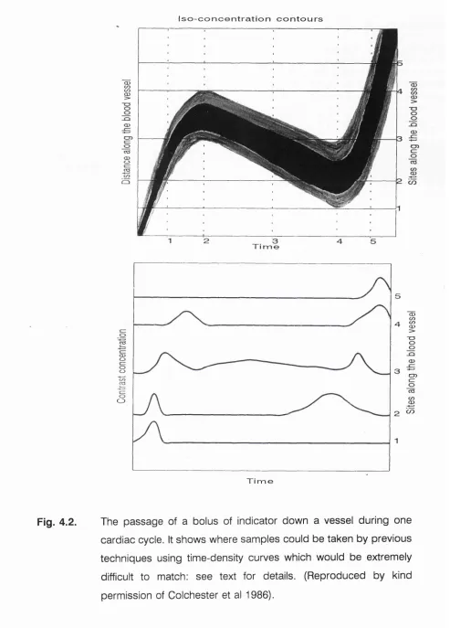
Fig. 4.2. The passage of a bolus of indicator down a vessel during one cardiac cycle. It shows where samples could be taken by previous

techniques using time-density curves which would be extremely

difficult to match: see text for details. (Reproduced by kind

permission of Colchester et al 1986).

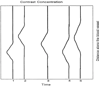
Fig. 4.3. Graphical representation of density-distance curves obtained from sites 1 to 5 from the image of a bolus of indicator down a vessel in

fig. 4.2.

Fig. 5.1. Diagrammatic representation of the factors involved in calculating blood volume flow. M and 0 are the vessel magnification factor and

the orientation of the blood vessel to the X-ray beam axis

respectively, t is the time taken for the contrast material bolus to

move a distance L along the vessel. X is the apparent length of the

vessel segment in pixels. The factor Kc is the product of the iodine

concentration in the vessel c and a densimetric calibration constant

K which relates the image grey value to the mass of iodine

integrated along the X-ray path from X-ray focus to image. The

integral of image intensity, a, is computed along the transverse

density profile after subtraction of a background or mask to remove

contributions from overlying and underlying tissues.

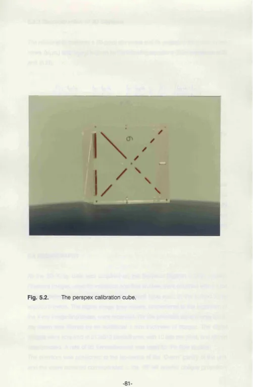
Fig. 5.2. The perspex calibration cube.

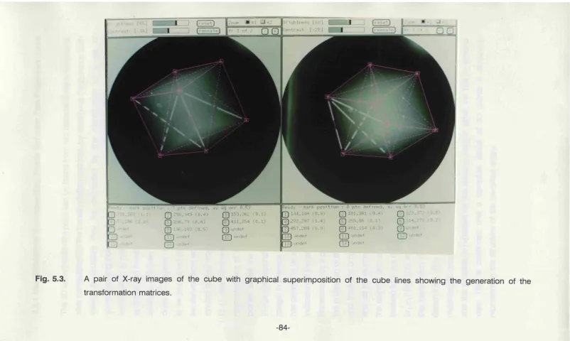
Fig. 5.3. A pair of X-ray images of the cube with graphical superimposition of the cube lines showing the generation of the transformation

matrices.

(12)

-9-Fig. 5.4. Graphic explanation of the definition of the epipolar line.

Fig. 5.5. Example of a landmark indicated in the right-hand view, plus the matching epipolar line in the left-hand view, on which the

corresponding projection has to be located. The images represent

the feeding vessel to the cerebral circulation of a patient in table 9.1

(MB).

Fig. 5.6. Schematic drawing shows how image blur affects automatic vessel edge detection. The maximum responses of the first derivative

operator underestimate the actual edge position while the maximum

responses of the second derivative operator overestimate the actual

edge position.

Fig. 5.7. A biplanar digital X-ray angiogram of the aortic arch and the major arteries leading towards the head, with the detected edges

superimposed on the angiograms (see table 9.1, patient MB).

Fig. 5.8. The true cross-section A is related to the integral of image intensity a along a profile perpendicular to the projection of the vessel axis.

The X-ray magnification factor M, angle 0 between the vessel axis

and the X-ray axis, and densimetric calibration constant K are

computed from the 3D reconstruction of the vascular configuration.

Fig. 5.9. Biplanar views of S’ shape wire phantom used to assess the accuracy of path length.

Fig. 5.10. Aluminium phantom used in the validation of the cross-sectional area study.

Fig. 6.1. Example of a series of 2D dynamic digital X-ray angiographic images. These images were acquired using the physical flow

phantom described in chapter 8. The tube calibre was 6.6 mm with

a mean blood flow of 349 ml/min. Images were acquired at a rate

of 25 frames per second.

Fig. 6.2. (a) Parametric image showing contrast medium concentration (grey scale) at different positions along the blood vessel (vertical axis) at

different times (horizontal axis), generated from 3D experimental

data acquisition for a 4.0 mm calibre with mean blood flow of 176

ml/min. (b) Graphic presentation of above parametric image shown

as three rows (30, 80, and 150 mm) of time-density curves.

(13)

1.04 seconds) of the parametric image in fig. 6.2(a).

Fig. 6.4. Graphical representation of the method for matching density- distance profiles over time.

Fig. 6.5. A example of the dependence of the mean sum of the square differences (MSSD) on the spatial shifts. The data demonstrate a

sharp minimum at a certain value of the shift. This value is taken to

be the distance transversed by the contrast material between the

two frames. Graphic presentation of the MSSDs are from the

parametric image shown in fig. 6.2 in four consecutive columns 25-

28 (1-1.12 seconds).

Fig. 6.6. A example of the cost function image, where the image grey level represents the mean sum of the square difference (MSSD) as a

function of time (horizontal axis) and shift (vertical axis) along a

vessel segment. The cost function image was generated by the

application of our velocity algorithm to the parametric image in fig.

6.2(a).

Fig. 7.1. Generation of a parametric flow image. The partially formed parametric image is shown on the left, while on the right there is a

graphical representation of the contrast concentration across the

diameter of the blood vessel lumen. The diameter of the vessel was

5 mm.

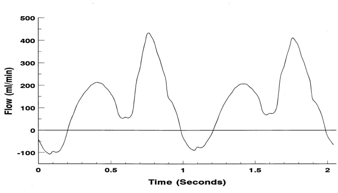
Fig. 7.2. Blood flow waveforms vs time used as input into the computer model.

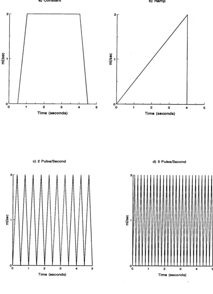
Fig. 7.3. Injection strategy for contrast medium in the simulation studies: (a) constant, (b) ramp, (c) 2 pulse/sec and (d) 5 pulse/sec.

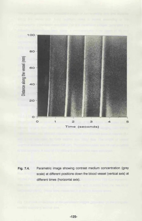
Fig. 7.4. Parametric image showing contrast medium concentration (grey scale) at different positions down the blood vessel (vertical axis) at

different times (horizontal axis).

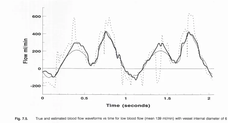
Fig. 7.5. True and estimated blood flow waveforms vs time for low blood flow (mean 139 ml/min) with vessel internal diameter of 6 mm. The

thin lines inputs the true waveform, the dotted lines that from the

bolus mass tracking algorithm (Swanson et al 1986) and the thick

lines the results using our velocity algorithm computing.

Fig. 7.6. True and estimated blood flow waveforms vs time for high blood flow (mean 650 ml/min) with vessel internal diameter of 6 mm. The

(14)

-11-thin lines inputs the true waveform, the dotted lines that from the

bolus mass tracking algorithm (Swanson et al 1986) and the thick

lines the results using our velocity algorithm computing.

Fig. 7.7. Plots of typical contrast concentrations vs time generated from synthetic data at two sites A (dotted lines) and B (solid lines), 40

mm apart, along a blood vessel with an internal diameter of 6 mm

and mean blood flow of 367 ml/min.

Fig. 7.8. Scatter plot showing the relationship between true mean velocity and mean velocity estimated by the tracking of bolus mass method

(Swanson et al 1986) for a 6 mm diameter vessel and a laminar

flow pattern. The results for ramp, constant, 2 and 5 pulse/sec

injection techniques are plotted. The line represents the line of

identity.

Fig. 7.9. Scatter plot showing the relationship between true mean velocity and mean velocity estimated by our velocity computing algorithm,

for a 6 mm diameter vessel and a laminar flow pattern. The results

for ramp, constant, 2 and 5 pulse/sec injection techniques are

plotted. The line represents the line of identity.

Fig. 7.10. Scatter plot showing the relationship between true mean velocity and the mean velocity estimated by the tracking of bolus mass

(Swanson et al 1986) for 2 and 4 mm diameter vessels with a

laminar flow pattern. The line represents the line of identity.

Fig. 7.11. Scatter plot showing the relationship between true mean velocity and the mean velocity estimated by our velocity computing

algorithm (distance-density curve matching method), for 2 and 4

mm diameter vessels, for a laminar flow pattern. The line represents

the line of identity.

Fig. 7.12. Scatter plot showing the relationship between true mean velocity and the mean velocity estimated by the tracking of bolus mass

(Swanson et al 1986) for a 4 mm diameter vessel for ‘plug’ or

constant axial flow pattern. The line represents the line of identity.

Fig. 7.13. Scatter plot showing the relationship between true mean velocity and the mean velocity estimated by our velocity computing

algorithm, for a 4 mm diameter vessel, for a ‘plug’ or constant axial

(15)

Fig. 8.1. Block diagram of flow phantom.

Fig. 8.2. Relationship between flow determined from timed fluid (saline) collection and the electromagnetic flowmeter (EMF) mean flow

reading.

Fig. 8.3. (a) Parametric image generated by 2D data processing for a 6.6 mm calibre with a mean blood flow of 348 ml/min. (b) Direct

comparison of volume flow waveforms measured synchronously

using the standard EMF (thin lines) and from the parametric image

using our velocity computing algorithm (thick lines).

Fig. 8.4. (a) Parametric image generated by 2D data processing for a 6.6 mm calibre with a mean blood flow of 708 ml/min. (b) Direct

Fig. 8.7. Direct comparison of volume flow waveforms measured synchronously using the standard EMF (thin lines) and from the

parametric image using our velocity computing algorithm (thick

lines) for a tube of 6.0 mm lumen diameter with a mean fluid flow

of 586 ml/min (parametric image generated by 3D data

processing).

(16)

-13-Fig. 8.9. (a) Parametric image generated by 3D data processing for a 4.0 mm calibre with a mean blood flow of 176 ml/min. (b) Direct

Fig. 8.12. Direct comparison of volume flow waveforms measured synchronously using the standard EMF (thin lines) and from the

parametric image using our velocity computing algorithm (thick

lines) for a tube of 3.0 mm lumen diameter with a mean fluid flow

of 229 ml/min (parametric image generated by 3D data

processing).

Fig. 9.1. X-ray angiogram showing the left femoral arteries. The arrows indicate the positions of the selected arterial segments for

generation of the parametric images, a= left common femoral;

b=left superficial femoral; and c=left profunda femoris arteries.

Fig. 9.2. Parametric image showing contrast medium concentration (grey scale) at different positions down the blood vessel (the vertical axis)

and at different times (the horizontal axis) pre-angioplasty for: (a)

the left common femoral, (b) the left superficial femoral with severe

stenosis and (c) the left profunda femoris arteries.

Fig. 9.3. As in fig. 9.2 but post-angioplasty.

Fig. 9.4. Plots of the flow velocity waveforms pre-angioplasty derived from the parametric images shown in fig. 9.2. The waveforms were

extracted from the parametric images constructed for the left

(17)

artery (dotted lines) and the profunda femoris artery (thin solid

lines).

Fig. 9.5. Plots of the flow velocity waveforms post-angioplasty. The waveforms were extracted from the parametric images shown in fig.

9.3 for the left common femoral artery (thick solid lines), the left

superficial femoral artery (dotted lines) and the profunda femoris

artery (thin solid lines).

Fig. 9.6. Parametric image showing contrast medium concentration (grey scale) at different positions down the blood vessel (the vertical axis)

and at different times (the horizontal axis), the left and right

common carotid (LCC, RCC), internal carotid (LIC,RIC) and

vertebral (LVE,RVE) arteries for patient MB (see table 9.3).

Fig. 9.7. Biplanar X-ray angiogram showing the carotid and vertebral arteries for patient MB (see table 9.3).

Fig. 9.8. Plots of the volume flow velocity waveforms. The waveforms were extracted from the parametric images shown in fig. 9.6 for the left

common carotid (LCC), right common carotid (RCC), left internal

carotid (LIC), right internal carotid (RIC), left vertebral (LVE) and

right vertebral (RVE) arteries.

(18)

-15-TABLES

Table 5.1. Computation of path length measurements after 3D reconstruction. Table 5.2. Table of the computation of the cross-sectional area A of holes

drilled in aluminium block.

Table 7.1. Example of input parameters used in flow model for laminar blood flow pattern.

Table 7.2. Measurements for the three different transport time methods of measuring mean blood flow at two sites 100, 50, and 25 mm

apart with a vessel of width 6 mm using time-density curves from

synthetic data.

Table 8.1. Summary of phantom experiments for 2D and 3D data processing. Table 8.2. Summary of results of phantom experiments with 2D data

processing.

Table 8.3. Effect of distance between injection site and measurement site on angiographic flow estimates using the experimental phantom, for an

internal tube diameter of 6.6 mm.

(a) Mean volume flow rate of 349 ml/min.

(b) Mean volume flow rate of 708 ml/min.

Table 8.4. The effect on angiographic flow estimates of reducing sampled length, for an internal tube diameter of 6.6 mm.

(a) Mean volume flow rate of 349 ml/min.

(b) Mean volume flow rate of 708 ml/min.

Table 8.5. Summary of results of 3D phantom experiments

Table 9.1. Summary of patient data of patients who have undergone head and neck DSA examination.

Table 9.2. Flow analysis from a 62-year-old female with minor right internal carotid artery stenosis.

Table 9.3. Summary of results from quantitative digital X-ray angiographic studies in patients who have undergone head and neck DSA

examinations. The table shows mean velocity V in mm/sec, cross-

sectional area A in mm^ and flow F in ml/min. # indicates that

vessel segments were too short to analyse. The results have been

computed for the left common carotid (LCC), right common carotid

(19)

vertebral (LVE) and right vertebral (RVE) arteries.

(20)

-17-ACKNOWLEDGEMENTS

The work presented in this thesis was carried out at several sites in the London

University Medical Schools. I would like to thank many people for their help

during the period of my research and in the production of this thesis.

First and foremost, I would like to thank Dr David J Hawkes for his supervision,

advice, encouragement and tremendous support throughout the last five years.

I also would like to thank my supervisor Professor K E F Hobbs who encouraged

and supported me in my travels around the London Medical Schools during the

performance of my research.

I would like to thank all within the Division of Radiological Sciences, United

Medical and Dental School, for their support, especially Martin Graves, Derek Hill,

Glyn Robinson and Cliff Ruff for assistance in the data handling and support of

the SUN station network. I am grateful to radiology and radiography staff at Guy’s

Hospital for their assistance in collecting the technical data.

I would like to thank all members of the University Department of Surgery, Royal

Free Hospital and School of Medicine, for their tolerance of my absences from

the department and their support and encouragement over the period of the

research on this thesis.

I would like to acknowledge the help of Dr Alan Colchester, Department of

Neurology, UMDS, who initially proposed the algorithms for computing blood

velocity and blood vessel cross-sectional area.

I would like to thank Mr C R Hardingham for writing the 3D reconstruction

program.

I acknowledge collaboration with Dr John Brunt of the Department of Medical

Biophysics at Manchester University and Professor George du Boulay of the

Institute of Neurology, Queen Square, London (who are investigating the use of

(21)

Many thanks to the Department of Medical Illustration at Royal Free Hospital for

photographing and printing some of the images from the computer screen.

Many thanks to friends and colleagues who proofread this thesis and gave me

much needed encouragement and support. Many thanks to Stewart Gray for

proofreading the final copy of my thesis.

(22)

-19-CHAPTER 1

INTRODUCTION

1.1 INTRODUCTION

In research and clinical practice there are many unresolved haemodynamic

problems for which quantitative measurements of blood flow could provide some

of the solutions. Methods of measurement of blood flow evaluate either tissue

perfusion or vascular blood flow. Tissue perfusion is the transmission of blood

through the microcirculation and is the ultimate determination of tissue

oxygenation; and is usually measured in ml/min/100 gram or ml/min/kg tissue

weight. The measurement of tissue perfusion is important in, for example,

monitoring tumour tissue perfusion and in dermatological and rheumatological

disorders. Vascular blood flow is a measure of the amount of blood passing

along a vessel; and is usually measured in ml/min. Applications include

assessment of the progression of atheroma, investigation of haemodynamics,

and study of the efficacy of vascular bypass operations and angioplasty. The

commonest type of vascular disease is atherosclerosis, which tends to affect

larger vessels. Measurement of flow or change in flow in the diseased vessel(s),

is a more direct assessment of severity of disease than measurements of tissue

perfusion in the region of supply of the vessel, which may be spatially ill-defined.

Several arteries may supply one territory (collateral supply). Vessel flow

measurement may however allow estimation of the relative contribution of

particular collateral vessels. Unfortunately no sufficiently accurate non-invasive

technique exists at present to measure vascular blood flow. In brief, currently

available methods include the electromagnetic flowmeter (EMF) which has been

used to estimate blood flow in animals and man. The technique is invasive,

requiring the placement of probes on blood vessels. Doppler ultrasound has

been used mainly for qualitative analysis of blood flow in vessels near the body

surface and can be used to measure aortic flow, but it lacks the necessary

resolution in space and time to assess smaller, deep-seated vessels. Magnetic

resonance techniques are developing rapidly, but present methods are time

consuming and have poor spatial resolution. X-ray angiography remains the

(23)

widely used in clinical practice for obtaining high quality blood vessel images. The

ability to derive quantitative flow data from this procedure would be a useful

clinical tool. Numerous publications have shown its potential but it has not been

widely used due in part, I believe, to the use of inappropriate algorithms to

process the image data.

The objective of this work is to examine the accuracy of using an X-ray

angiographic technique to compute blood flow. Hence it concentrates on the

derivation and subsequent processing of blood flow waveforms from digital

dynamic X-ray angiographic data. It is therefore a methodological study rather

than a clinical study. Although limited patient data were acquired and analysed

these have mainly been used to demonstrate that the theory and methods

developed using synthetic and phantom data may be applicable in clinical

studies.

This chapter includes an outline of applications of blood flow measurements, with

special reference to arterial blood flow waveform patterns in the detection of

vascular diseases. This is followed by a breakdown of the thesis as a whole,

chapter by chapter.

1.2 APPLICATIONS OF BLOOD FLOW MEASUREMENTS

Blood flow measurements in individual vessels would be of value in a variety of

clinical circumstances:

(1) To confirm the clinical diagnosis.

(2) To achieve a better understanding of the patho-physiology of the disease

process.

(3) To document the progression of the disease, for example: (a) the

assessment of the effect of atherosclerosis and other sources of vessel

narrowing on flow in individual vessels (b) the study of hepatic blood flow

for better understanding of the natural history of portal hypertension.

(4) To measure total blood flow to an organ, pre and post kidney or liver

transplants.

(5) To predict pressure gradients from the combination of vessel blood flow

(24)

-21-measurements with calibre and path length -21-measurements.

(6) To assist the selection of patients for reconstructive surgery.

(7) To assess the immediate and long-term post-operative results of

reconstructive surgery, such as the investigation of bypass graft patency.

(8) To assess the haemodynamic effects of percutaneous transluminal

angioplasty and other interventional studies.

(9) To assess changes in pulsatile flow waveforms in vascular disease. This

is discussed in section 1.2.1.

(10) Finally, there is still much to be learnt about the physics, physiology and

pathology of blood flow and vascular resistance in individual vessels.

Flow measurements in individual vessels are a central part of this research.

1.2.1 Arterial Flow Velocity Waveform Patterns

The pattern of flow waveforms can be used to grade the severity of arterial

occlusive disease. Individual vessels have different blood flow waveform patterns

depending on their location. For example:

(1) The normal flow pattern in the major arteries of the lower limb consists of

an initial high-velocity forward-flow phase during cardiac systole, a brief

phase of reverse flow in early diastole, and a low-velocity forward-flow

phase in late diastole. The factors that modify this normal pattern include

the presence of arterial occlusive disease and changes in peripheral

vascular resistance. An arterial stenosis acts like a filter which removes

rapidly changing components of the flow waveform. This, together with the

compensatory decrease in peripheral resistance, results in the

disappearance of the reverse-flow phase (see chapter 9). Thus, the

waveform obtained distal to a stenotic lesion has a single forward velocity

phase, the peak flow velocity is lower than normal and the peak of the

waveform is more rounded. Flow waveforms taken from within a

haemodynamically significant stenosis have an abnormally high peak

systolic velocity that represents the high-velocity jet generated due to the

lesion.

(25)

normally show forward flow throughout the cardiac cycle and relatively

high diastolic flow velocities (see chapter 9).

1.3 STRUCTURE OF THESIS

Chapter 2 critically describes current available methods for measuring blood flow,

emphasising their difficulties and relative advantages.

From the review of the literature in chapter 2, it is apparent that there are many

problems associated with determining blood flow. X-ray angiography remains the

imaging modality which gives the highest spatial and temporal resolution, and,

because of its high signal-to-noise ratio, is widely used in clinical practice for

obtaining high-quality vessel images. In addition to conventional anatomical

information, a timed sequence of digital images also contains useful temporal

information which hitherto has been largely ignored.

Chapter 3 describes the main principals of a digital X-ray angiographic system

and outlines its individual components.

Chapter 4 discusses in detail the drawbacks of the existing X-ray angiographic

techniques of measuring blood flow velocity, introduces approaches to the

measurement of pulsatile blood flow waveforms from profiles of injected contrast

mass or concentration versus distance, and outlines outstanding problems in

their implementation. In this chapter X-ray angiographic techniques to measure

cross-sectional area are reviewed emphasising both the value and shortcomings

of using geometric or densitometric methods to calculate the cross-sectional

area.

Chapter 5 describes in detail a three-dimensional (3D) reconstruction technique

for obtaining vascular configurations from biplanar X-ray angiographic images.

Such reconstruction is possible on condition that the position and orientation of

the X-ray equipment during the data acquisition is known, and that corresponding

vessel segments in the vascular configuration in the two projections can be

identified. This chapter also includes a validation of the 3D approach for the

measurement of vessel cross-sectional area and vascular path lengths.

(26)

-23-Chapter 6 describes a new digital X-ray angiographic technique of measuring

blood flow waveforms, by matching profiles of injected contrast concentration

with respect to distance along a blood vessel (distance-density curves) over a

period of time.

Two procedures will be described, in chapters 7 and 8 respectively, that validate

the new flow algorithm. The first method uses simulated X-ray angiographic data

generated by computer models (details and results of the validation are

described in chapter 7). Quantitative comparison with other algorithms is also

made using computer generated images. A total of 114 synthetic images were

generated by varying the following parameters in the mathematical model of the

angiographic imaging chain; flow rate, blood vessel calibre size and injection

technique (chapter 7). The second method is a validation of the technique using

an experimental model of blood circulation. The results obtained from this system

are described in chapter 8.

In order to demonstrate the applicability of the new angiographic technique (as

described in chapter 6) in clinical practice, flow was measured in the left femoral

arteries of a 69-year-old male patient with severe superficial femoral artery

stenosis, pre- and post-percutaneous transluminal angioplasty and, subsequently,

in the carotid and vertebral arteries of seven patients. The analysis of the flow in

the femoral artery was performed using two-dimensional (2D) image processing,

in the plane of the projected radiograph, while the analysis of the vessels in the

head and neck was performed using a 3D representation of the vascular network

(chapter 9).

The tenth and final chapter provides the conclusion and overall assessment of

(27)

CHAPTER 2

A REVIEW OF EXISTING METHODS OF MEASURING FLOW IN BLOOD VESSELS

The measurement of blood flow is important in understanding both normal

physiology and disease processes as well as assessing the effects of therapeutic

procedures such as angioplasty, shunting, bypass and transplantation.

There are several techniques which have been used to measure blood flow. The

classification of techniques is to some extent arbitrary and several so-called

‘different’ methods may share certain common principles. The methods can be

classified into two main groups: those primarily concerned with flow through

discrete vessels and those used to assess local microcirculatory blood flow

(tissue perfusion). All techniques have their advantages and disadvantages and

in some situations a combination may provide the most information (Seifalian et

al 1991a). In addition, because of the many factors affecting blood flow,

measurement in a single subject may vary depending on position, recent food

intake, anxiety, anaesthesia and drug therapy. This thesis does not attempt to

address these external factors, rather it addresses the technical problem of

measuring flow through discrete vessels. The development of a technique to

measure intravascular blood flow using digital X-ray angiographic data is

described. The technique of digital X-ray angiography is described in chapter 3

and previous approaches to using these data to measure flow are reviewed in

chapter 4. This chapter surveys other methods available for assessing

intravascular blood flow, examines the different parameters being measured, and

outlines problems of applicability and interpretation of the results from each

technique.

(28)

-25-2.2 METHODS

2.2.1 The Electromagnetic Flowmeter

The measurement of blood flow by electromagnetic induction was first suggested

by Fabre in 1932. The principle of the technique is based on Faraday’s law of

electromagnetic induction. If a magnetic field is applied across a vessel in which

blood is flowing then an electric field is induced at right angles to both the

induced magnetic field and the flow vector (Webster 1978; Harper et al 1974).

The electrical field is detected along its axis from the potential difference across

the outside of the vessel. This potential is primarily determined by the velocity of

the flowing blood within the vessel. Accuracy demands attention to detail and

proper calibration (Khouri and Gregg 1963; Wyatt 1984) using a pump and saline

solution. There is no way of checking calibration ‘in-vivo’ except by vessel

clamping for zero flow. Interference from other electrical instruments also reduces

the accuracy of the technique (Meisner and Messmer 1970).

In practice the method involves the placement of the device around the vessel to

be assessed. For a good signal, close contact is essential. Drapanas et al (1960)

and Price et al (1965) compared electromagnetic flowmetry with the

bromsulphalein clearance method (Bradley et al 1945) for measuring hepatic

arterial and portal vein flow in a dog and found a good correlation between the

two methods. Because of the invasive nature of the technique, it is applicable

mainly to animal studies and to patients at the time of surgery. These devices are,

however, still regarded as the ‘gold standard’ against which all other methods of

measuring flow must be compared. Electromagnetic flowmeters are able to

measure instantaneous and mean blood flow in an exposed vessel. They can

also detect forward and reverse flow and the temporal resolution is fast enough

for flow to be studied during the cardiac cycle. Another advantage of this method

is its insensitivity to changes in blood temperature and viscosity.

2.2.2 The Thermodilution Technique

The concept of the thermodilution technique is based on the principle of

(29)

the blood temperature at a point downstream. The rate of the injection washout

is proportional to the flow. Fegler (1954) injected heated saline solution (the

indicator) into the blood stream via a catheter, then applied the Stewart-Hamilton

equation (Hamilton et al 1932), describing the relationship between injected

volume, the area under the time-dilution curve, and blood flow in thermodilution

techniques:

P_ ^*(7b T)*SO*K (2.1)

where F is blood flow, 0 is the injected indicator volume, and Tj are the blood

and injected indicator temperatures, A is the area under the temperature time

curve and K is the fluid constant. The fluid constant is dependent upon specific

gravity and heat of blood and indicator, it remains virtually constant and is

calculated to be equal to 1.08 when isotonic saline or 5% dextrose solution is

used (Nadel et al 1986).

Nadel et al (1986) validated this technique ‘in-vitro’ for flow ranging from 200 to

700 ml/min, and reported that flows under 200 ml/min had an average error of

28%, while flows above 200 ml/min had an average error of 6%.

The assumptions for this technique are that there is homogeneous mixing

between the indicator and the blood, and that the injection of the indicator does

not influence flow. Apart from the mixing problem, one of the difficulties of the

injection technique is that heat is lost from the fluid during its passage to the

catheter tip and this heat passes out into the blood altering its temperature and

therefore the temperature recorded by the downstream sensor. In addition

injection of hot or cold saline might affect the vascular tone of arteries and hence

the arterial blood flow.

2.2.3 Doppler Ultrasound

According to the Doppler principle, the frequency of a sound wave that is

reflected from a moving object will increase or decrease depending on the

(30)

-27-object’s direction and velocity relative to the incident wave. This change in

frequency is called the Doppler effect. Using ultrasonic equipment the Doppler

shift ôF is given by the following equation:

where F is the transmitted frequency (2-10 Mhz), V is the velocity of the moving

blood cell, 0 is the angle between the transmitted sound and the axis of blood

vessel and c is the constant speed of sound in the blood and tissue (« 1540

m/sec).

Doppler instrumentation allows for ultrasound to be transmitted continuous wave

(CW) Doppler or intermittent (pulsed) wave Doppler.

The advantage of the CW Doppler is its simplicity, no upper limit to the velocity

measurable, and a lack of aliasing. Therefore CW Doppler may be used for the

analysis of high velocities, particularly across stenotic orifices. These devices are

commonly used in obstetrics to obtain umbilical artery waveforms, and have been

widely used for many years in the carotid and lower limb arteries.

The disadvantages of the system are that it does not allow determination of the

depth at which the frequency shift occurred, it provides little information about

flow profile and it is unable accurately to measure a detected stenosis (O’Leary

1985).

In pulsed wave Doppler, several intermittent gated (timed) voltage pulses are

applied to the transducer, resulting in a pulsed, rather than continuous, wave

transmission. Pulsed Doppler devices usually have a single crystal, operating

alternately as transmitter and receiver. The principle of operation is to transmit a

short burst of ultrasound towards the target and wait for the backscattered

ultrasound to return. By selecting the time between transmission and reception,

the depth at which blood velocities are detected can be chosen. This provides

(31)

of moving interfaces and scatterer from within a well-defined ‘sample volume’.

The dimensions of the sample volume are defined axially by the pulse length and

laterally by the beam width of the combined transmitter-receiver system. The

sample volume can be positioned anywhere along the axis of the ultrasound

beam, but to obtain a narrow band of frequencies it should be placed in the

central stream of the blood vessel (Breslau 1982).

While pulsed Doppler has the considerable advantage of permitting Doppler

analysis at precise locations determined by the operator, there are velocity

measurement limitations. The highest velocity that can be detected is a function

of the transmission frequency, the depth at which the velocity is sampled, and the

intercept angle. Altering the intercept angle away from parallel flow may permit

velocity measurements that can be corrected to the true velocity by multiplying

by the cosine of the intercept angle. Difficulties, however, arise in measurement

of the intercept angle.

With simple Doppler ultrasound alone, details of flow are obtained but the vessel

and surrounding soft tissues cannot be evaluated and so there is no anatomic

reference. Placing the sample volume at a desired anatomical site requires the

combination of an imaging device with a Doppler device and is referred to as

duplex scanning.

Most commonly, duplex probes contain two piezoelectric transducers positioned

in a geometric configuration that allows simultaneous real time sector imaging

and pulsed Doppler flow studies (Burns 1987). Therefore it has the advantage of

both Doppler spectral analysis and real time imaging which enables the

measurement of volume flow in blood vessels. Volume flow is the product of

cross-sectional area and mean velocity. The vessel area is estimated from the B-

scan, and the mean velocity estimated from the mean velocity shift of the Doppler

spectrum. The limitation of the technique is due to the conflict between design

considerations optimal for imaging and those that are optimal for Doppler

measurement. Doppler frequency shifts are maximal when the axis of the

transducer is as near parallel to the axis of flow as possible, whilst imaging is

best when the beam axis is perpendicular to the vessel wall. These design

constraints make simultaneous collection of Doppler and imaging data difficult.

(32)

-29-Although duplex instrumentation is now widely accepted as valid for most

vascular applications, there are several disadvantages which have prevented total

acceptance of the method (Jaffe 1984). These have been well documented and

are summarised by Burns (1987) and Merritt (1986). Briefly, they are as follows:

(a) Sampling problems. When used to measure laminar flow in a vessel with

a beam width less than the diameter of the vessel, only the central portion

of the vessel lumen will be insonated (Evans 1982 and 1986) leading to an

error in estimating velocity and hence flow. Nearly all current pulse mode

Doppler machines are based on centre-line measurements of peak velocity

and spectral broadening (Langlois et al 1984). Abnormalities may be

missed due to failure to sample nearer the wall where flow disturbances

are more likely to occur (Switzer and Nanda 1985; Rittgers and Fei 1988).

(b) Errors can arise in estimating blood vessel diameter. These are due to

imaging not being perpendicular to the longitudinal axis of the vessel;

poor resolution of the imaging transducer; pulsatility of blood flow, causing

variation in vessel diameter with time; and observer variability (Zoli et al

1986). Assuming that a vessel is circular can lead to an error of up to 30%

in calculating the area of the vessel (Gill 1985).

(c) Errors due to beam angle. The magnitude of velocity is a function of the

cosine of the intercept angle between beam direction and the blood

vessel. The volume flow rate calculation equation is a trigonometrical

function of the angle between the beam direction and the blood flow.

Errors vary considerably with that angle, being minimal in the angle range

55-75° (Stacey-Clear and Fish 1984).

To overcome problems of visualisation of flow in small vessels and to improve

qualitative analysis, colour-duplex instruments have been developed (Nelson and

Pretorius 1988; Fowls 1988). Colour-duplex imaging instruments provide the

following additional information: (1) with the existence of a Doppler frequency

shift, the echo is represented in colour otherwise it is displayed in shades of grey,

(2) the magnitude of the Doppler frequency shift is displayed on a colour shading

scale, with the direction of blood flow, with reference to the Doppler transducer,

(33)

The advantages of the colour-duplex is the resultant visualisation of flow, even if

the vessel is too small to be resolved on the grey-scale image, and distinction

between vascular and non-vascular structures, for instance at the portal hepatis

where blood vessels can be distinguished from the extrahepatic bile ducts. It is

important to recognise that the flow information illustrated with colour-duplex

instruments is qualitative, not quantitative (Zwiebel 1990).

To overcome problems with angle correction and sampling error in duplex

ultrasound systems, intra-arterial Doppler catheters have been used to measure

blood flow (Wilson et al 1985; Sibley et al 1986). The Doppler catheter has a

single crystal mounted 4.5 mm behind the catheter tip and angled at 45° to the

long axis of the catheter.

Intra-arterial Doppler catheters are frequently used in the coronary circulation

(Sibley et al 1986; Johnson et al 1989), but recently have been used to measure

flow in the superior mesenteric artery in patients, with and without portal

hypertension, who are undergoing diagnostic splanchnic arteriography

(McCormick et al 1992).

We have validated an intra-arterial Doppler ultrasound catheter to test for its

accuracy in quantitative measurement of pulsatile blood flow velocity. An

experimental model of the arterial circulation was constructed. This consisted of

a pump, flexible plastic tubing, and the tubular probe of an EMF (McCormick et

al 1992).

In the flow model the catheters were able to reproduce the flow velocity

waveforms for a 6.5 mm calibre tube but tended to overestimate the

instantaneous flow velocity by an amount ranging from 5.3% to 36.4%. The

results showed much poorer agreement for smaller calibre tubes (4.5 and 3.0

mm) in which the errors were as high as 200% (Seifalian et al 1991b). Similar

results were observed in the patient femoral artery undergoing bypass graft using

intra-arterial Doppler ultrasound and comparison with EMF reading.

In summary, all Doppler devices are subject to the same physical constraints;

even the most sophisticated colour flow mapping systems are subject to aliasing

(34)

-31-and the angle dependence of the Doppler shift frequency. Duplex scanning

potentially provides a non-invasive way of assessing blood flow in many clinical

situations. Its accuracy has been validated ‘in-vitro’ and in experimental animals

(Miyatake et al 1984; Seifalian et al 1988a), but problems do exist in using this

technique in clinical practice.

2.2.4 Nuclear Magnetic Resonance

Nuclear Magnetic Resonance (NMR) imaging is a non-invasive imaging modality

that has rapidly gained clinical acceptance, although widespread introduction has

been delayed by the capital cost of installing a NMR scanner. Flow detection with

NMR has been explored for more than 40 years (Suryan 1951 ; Garroway 1974;

Hahn 1960). When NMR imaging was first performed in the late 1970s, signal loss

was noted within arteries and attributed to high flow rates (Hawkes et al 1980).

In the early 1980s, several causes of increased signal intensity were described,

generally associated with slow flow in veins and durai sinuses (Waluch and

Bradley 1984; Bradley and Waluch 1985). Understanding these flow phenomena

has provided the basis for the development of specialised NMR imaging

sequences intended to quantify blood flow measurements. Several methods have

been proposed to quantify blood flow (Ridgway et al 1987; Shimizu et al 1986;

West et al 1988) and a full review of the techniques is described by Smith (1990).

The theory of applications of NMR to measure blood flow is too complex to

describe in full here. However, in brief, there are three main approaches to the

measurement of blood flow using NMR: (1) measurement of the signal produced

by the inflow and outflow of blood in an image selected perpendicular to the

vessel axis, (2) time-of-flight techniques, where a bolus of blood is used as an

indicator: it is excited and then its progress along the vessel is followed, and

finally (3) phase modulation, which utilises the phase of the net magnetic

moment. At present the relative merits of each approach in terms of spatial and

velocity resolution and image acquisition times have not been completely

evaluated. However, this will undoubtably be an area of significant development

(35)

2.3 CONCLUSION

Currently the measurement of blood flow is difficult. There are often large

variations in flow measurements between techniques. Some of these differences

may be due to the methods and conditions used while others are undoubtedly

caused by complexities of the blood flow in the vascular system which are not

yet completely understood.

Most importantly, a reliable method of non-invasively assessing blood flow in the

clinical context is still required. Duplex Doppler ultrasound offers a non-invasive

way of assessing blood flow but its many inaccuracies make it a difficult

technique to use in quantitative studies, especially when studying deep seated

vessels such as abdominal or cerebral arteries. Intra-arterial Doppler flow probes

and NMR may have a role in the future.

In chapter 4, X-ray angiographic techniques of measuring blood flow are

reviewed. In chapters 5 and 6 a new technique to measure blood flow using

digital X-ray angiographic data is introduced.

(36)

-33-CHAPTER 3

PHYSICS AND INSTRUMENTATION OF DIGITAL ANGIOGRAPHY

Over the years, X-ray film with an intensifying screen has proved to be an

excellent medium for the detection and display of images in the majority of

conventional radiographic examinations. However, printing the images on film

presents several limitations that are becoming more important as interventional

techniques make greater demands on X-ray imaging. The first of these limitations

is that images are generally not available on cine-film until approximately 15-20

minutes after the procedure compared to two minutes for single X-ray film. As a

result, the images cannot be used to guide an interventional study unless the

procedure is interrupted for film processing. In addition, the adequacy of the

images is not known until film development, so more views than necessary may

have to be obtained at a cost of increased contrast dose, radiation exposure, and

time.

Other problems related to the use of film are technical, including; the limited

dynamic range of X-ray film; a non-linear relationship between optical density and

exposure; the inconvenience of film digitisation necessary for most quantitative

analysis; and lack of control over image contrast after acquisition.

To overcome these problems, digital radiology has been developed. The basic

principle of digital imaging is that an image is stored as rectangular array of

numbers, each number relating to image intensity at that point. This digital image

can be manipulated or analysed by computer. The numbers are either converted

back into a visual image for viewing or quantitative data may be generated such

as cross-sectional area of a blood vessel, volume of a particular structure, and

flow rate down a blood vessel, etc.

3.2 PRINCIPLES OF DIGITAL FLUOROGRAPHIC IMAGING

A simplified block diagram of the processes involved in digital fluorography is

shown in fig. 3.1. The whole system is controlled by a general-purpose computer.

(37)

x-ray tu b e P atient

Im age Intensifier

Video C am era

ADO

C om p u ter

light I

X -ray

Computer Controlled Aperture _{to data storage}

a n alog signal and p ro c e s s in g

Fig. 3.1. Block diagram of basic system used for digital fluorography. The main imaging components include: X-ray tube, image

intensifier, video camera, high speed analogue-to-digital converter (ADC), and a computer.

(38)

-35-3.2.1 X-ray Tube and Generator

The standard features and requirement for X-ray sources are well known (Leeuw

1986). In summary, diagnostic application requires: (1) high instantaneous power

levels up to 100 Kw, of a short duration; (2) highly stable voltage during each

exposure, this is critical for studies which evaluate the temporal variations of

contrast material such as vascular flow; (3) provision for pulsing the radiation

source at up to 50 pulses per second, short X-ray pulses are essential to avoid

blurring of moving structures; (4) a small ‘focal spot' to maximise geometric

sharpness, because the spatial resolution of images depends on the type of

image receptor, the magnification factor, and on the actual focal size of the X-ray

tube. Typical focal spots are 0.2-0.6 mm. These X-ray systems can therefore

provide diagnostic images for visual interpretation and, in addition, quantitative

densitometric data can be derived.

An important factor in digital angiography is the synchronisation of the X-ray

generator with the digital video processor. Different systems accomplish this

differently; the Siemens Digitron II digital subtraction angiographic (DSA) system

used in acquiring the digital X-ray angiographic data used in chapters 8 and 9,

use the following methods for synchronising the X-ray exposure and T.V. scan

sequence. At 25 frames per second the X-ray exposure is typically 4 ms which

is immediately followed by the scan of the T.V. target. The system controller

synchronises both X-ray exposure and T.V. scan sequence to mains frequency.

At 50 frames per second the exposure times are shorter and only one scan of

an interlaced sequence (312 lines) is used.

3.2.2 Image Intensifier

The primary radiological image may be converted instantaneously into a visual

image by use of an image intensifier (II). A detailed description of the II has been

written by Nalcioglu et al (1986) and Fujita et al (1985). In brief an II has an input

phosphor and photocathode, where X-ray photon energy is converted into light

energy and hence a release of electrons. The electrons are accelerated by a high

voltage and are focused on to an output phosphor, where the electrons are

(39)

conversion process, so that for every X-ray photon arriving at the input phosphor

of the intensifier, many thousands of light photons are generated at the output.

Three major factors define the quality of an II:

(1 ) quantum detection efficiency (ODE), this measures the accuracy or quality

of data transfer in imaging systems and is defined as:

(3.1)

QDE=

iSNRJ

where SNR-^^ and SNR^^j^ are the signal-to-noise ratio in and out

respectively;

(2) spatial resolution, and

(3) field of view.

The thicker the input phosphor of the II, the higher the ODE, but the poorer the

spatial resolution; typical values for efficiency are 50% at 50 kev. The spatial

resolution varies with field size, typical values are 2 to 5 Ip/mm full width half

maximum (FWHM) for a field size of 110-400 mm. The other important parameter

in assessing quality is geometric distortion. Limitations in the electron optics lead

to distortion in the II during the acceleration of electrons from the input phosphor

to the output phosphor and due to the curved face of the input phosphor

(Chakraborty 1987). This results in a pincushion distortion effect. The result of this

distortion is that images are stretched in the radial direction by a factor which

increases as the distance from the centre of the image increases. Although it

does not degrade the resolution significantly, it may produce error in geometric

measurements. This distortion can usually be corrected by imaging a calibrated

metallic grid and by applying the subsequent corrections. In a modern II this

effect is very small, and we have shown that it can be considered to be negligible

in geometric measurements (see chapter 5).

(40)

-37-3.2.3 Video Camera

This is the single most important element in the imaging chain. A video camera,

more usually of vacuum-tube design, is coupled to the output screen of the

image intensifier by a lens system. The primary function of the system is to

convert the light intensity image (optical image) produced by the II to an

electronic signal that can be digitised. Some of the important properties of the

video camera are:

(1) speed of acquisition (frame rate);

(2) signal-to-noise ratio (SNR);

(3) linearity between output video signal and the incident X-ray flux, which is

determined by the photoconductivity of the target material used (Sandrik

1984);

(4) spatial resolution;

(5) extent of the ‘blooming effect', whereby if a high intensity object is

adjacent to a low intensity object, there is in effect some leakage of the

high intensity area onto the lower intensity area.

State of the art cameras such as a Plumbicon*^* (lead oxide) have a resolution

of 1249 or 525-lines for a 1024x1024 or 515x512 pixel matrix respectively, and a

SNR of 1000:1 or better, with an acquisition rate of 25 or 30 frames per second

(Roehring et al 1981). Other advantages of the lead oxide are that the output

video signal is linearly dependent upon the incident X-ray flux (light intensity);

whereas, for other types of video camera the video output V is approximately

related to the light flux I according to the relationship

V = r (3.2)

where r is a constant. For the Plumbicon camera (lead oxide) r« 1 , whereas for

typical non-linear fluoroscopic cameras (such as those with an antimony trisulfide

target) r= 0 .6 (Kruger et al 1981a). For digital imaging, a value of r= 1 is needed

for accurate subtraction and quantisation. Before the digital image is displayed