Study Of Heat Transfer By Mhd Flow Near The Stagnation Point Over A Stretching Sheet In Fuzzy Environment

(1)

IJSRR, 7(4) Oct. – Dec., 2018 Page 2456

Research article Available online www.ijsrr.org

ISSN: 2279–0543

International Journal of Scientific Research and Reviews

Study Of Heat Transfer By Mhd Flow Near The Stagnation Point Over

A Stretching Sheet In Fuzzy Environment

1

Saikia

Raphel Kumar

*

and

2

G C Hazarika

1

Department of Mathematics, Jorhat Institute of Science & Technology, Jorhat, Assam, India

2

Department of Mathematics, Dibrugarh University, Assam, India

ABSTRACT

A numerical investigation is done to study an MHD flow near the stagnation point over a stretching sheet with heat transfer. The governing partial differential equations with the boundary conditions are fuzzified using Zadeh’s extension principle. The fuzzified governing equations along with the fuzzified boundary conditions are solved numerically using fourth order Runge-Kutta shooting method. The values of velocity and temperature for different involved parameters are tabulated.

KEYWORDS:

MHD flow, stagnation point, fuzzy environment, triangular fuzzy number, extension principle.

*Corresponding author

Saikia

Raphel Kumar

Department of Mathematics,

(2)

1. INTRODUCTION

The practical applications of the dynamics of fluid flow over a stretching surface are of utmost importance such as extrusion of plastic sheets, glass blowing, paper production, drying of papers and textiles, drawing plastic films, metal spinning, continuous casting and spinning of fibres etc. Since the quality of final products depends to a large extent on the skin friction coefficient and the surface heat transfer rate, so in all of the above cases, a study of the flow field and heat transfer can be significant importance. Many researchers have investigated various aspects of this problem, such as consideration of mass transfer, exponentially stretching surface, magnetic field and application to non-Newtonian fluids, and similarity solutions have been obtained.

Initially, Sakiadis1 presented the boundary layer flow on a moving continuous solid surface. Later, Crane2 studied a closed form solution of the two-dimensional flow over a stretching sheet by considering the stretching velocity proportional to the distance from the slot. The problems of the flow through stretching surface have been investigated by Wang3, Troy et al.4, Vajravelu and Nayfeh5, Mukhopadhyay and Andersson6 and Jat and Chaudhury 7 in various conditions. Makinde and Aziz 8, Mahapatra et al.9 and Chaudhury et al. 10 analyzed the flow over stretching surface in different cases.

Stagnation point virtually appears in all flow fields of engineering and science, so stagnation point flow is a topic of significance in fluid mechanics. The stagnation region encounters the highest heat transfer, the highest pressure and highest rate of mass decomposition. Stagnation pont flow has various applications in many manufacturing processes in industry. The applications include the boundary layer along material handling conveyers, the aerodynamic extrusion of plastic sheets, blood flow problems, processes in the textiles and the paper industries, flow over the tips of rockets, aircrafts, submarines and oil ships. The pioneering work in this area was carried out by Heimenz 11 who studied the steady boundary layer flow in the region of a stagnation point on an infinite wall. The extension to the axisymmetric case was presented by Homann12. Later, a large number of analytical and numerical studies explaining various physical situations of the boundary layer stagnation point flow are presented by Sparrow et al. 13, Chiam 14, Amin and Riley 15, Mahapatra and Gupta 16 and Wang 17. Most recently, Rosali et al. 18, Mahapatra and Nandy 19 and Lok and Pop 20 considered the problem of stagnation point flow in various situations.

(3)

media, namely, petroleum reservoir operations, food processing, ooling of nuclear reactors, building insulation, underground disposal of nuclear waste, and casting and welding in manufacturing processes. Enhancement of forced convection by the use of a porous substrate has been the subject of several investigations. Comprehensive references on flow in porous media can be found in books by Ingham and Pop 21, Schlichting and Gersten 22, Vafai 23 and Nield and Bejan 24. Moreover, Vafai and Kim 25 reported a composite system problem involving a relatively thin porous substrate attached to the surface of a flat plate.

In recent years, a number of simple fluid flow problems of viscous incompressible fluid have attained new attention in the more general context of magnetohydrodynamics. The desired properties of the end product and the rate of cooling can be controlled by the use of electrically conducting fluid and applications of magnetic field. The study of magnetohydrodynamic flow through a heated surface has important applications in many technological processes such as exotic lubricants and suspension solutions, magneto-hydrodynamic flight, foodstuff processing, MHD power generators, solidification of liquid crystals, the boundary layer control in aerodynamics, and in the field of planetary magnetosphere. Hydromagnetic boundary layer flow over a stretching surface has attracted attention of many researchers in recent time due to its important applications in metal-working processes and modern metallurgy. It seems that the magnetohydrodynamic flow over a stretching surface was first investigated by Andersson 26. On the other hand, the problem of MHD stagnation point flow past a stretching sheet was presented by Mahapatra and Gupta 27. Later, Abel and Mahesha 28, Ramesh et al.29, Singh and Singh 30, Makinde et al. 31, Olajuwon and Oahimire 32, and Chaudhary and Kumar 33 analyzed and presented MHD flow problems considering various aspects of the problems.

In this article, an attempt has been made to fuzzify boundary value problems by taking an

MHD flow problem near the stagnation point over a stretching sheet. We have observed the velocity

and temperature distribution after fuzzifying the governing equations by Zadeh’s extension principle.

The fuzzified ordinary differential equations along with the fuzzified boundary conditions are solved

by using fourth order Runge-Kutta shooting method by formulating suitable computer programs in

MATLAB.

2. BASIC CONCEPT OF FUZZY SET THEORY

a.

Fuzzy Sets and Membership Function:

Let X be a universal set. A fuzzy set ̃ in X is characterized by its membership function denoted by ̃, i.e.,

̃ , -

(4)

IJSRR, 7(4) Oct. – Dec., 2018 Page 2459 If * + is a collection of objects denoted generically by x, then a fuzzy set ̃ in X is a set of ordered pairs

̃ {( ̃( )) }

where each pair ( ̃( )) is called a singleton.

b.

Fuzzy Number

16

:

A fuzzy number is a convex normalized fuzzy set defined on whose membership function

is piecewise continuous.

A triangular fuzzy number A can be defined as atriplet , -. Its membership function is defined as:

( ) {

A trapezoidal fuzzy number A can be expressed as , -and its membership function is defined as:

( )

{

c. Zadeh’s Extension Principle 34:

A crisp function is said to be fuzzified when it is extended to act on fuzzy set

defined on X and Y. i.e.,

̃ ̃ ̃ and its inverse has the form ̃ _{̃ ̃.}

The extension principle states that for a given crisp function there induces two

functions ̃ and ̃ _{which are defined above for which membership functions are given by}

_{[ ̃( )]( )} _{( )} ( ), for all ̃

and _{[ ̃} _{( )]( )} ( ̃( )), for all ̃.

3. DESCRIPTION OF THE PROBLEM

We consider a steady, two-dimensional stagnation point flow of a viscous incompressible electrically conducting fluid impinging normally on a stretching surface of a constant temperature

(5)

varies linearly along x-axis, i.e., ( ) , where is the strength of the stagnation flow. The ambient fluid temperature is constant. It is assumed that the velocity of the stretching surface is

( ) , where is the stretching rate.

Fig, 1: Flow configuration

With the above assumptions the governing boundary layer equations are:

( )

( ) ( )

(

)

( ) ( )

Boundary conditions are-

( )

( ) } ( )

where u and v are the velocity components in the x and y directions respectively, is the kinematic viscosity, is the permeability of the porous medium, is the electrical conductivity, is the fluid density, T is the temperature of the fluid, is the thermal diffusivity, is the coefficient of viscosity and is the specific heat at constant pressure.

To transform the above governing equations into ordinary differential equations, following similarity transformations are introduced.

( ) √ ( ) ( )

√

(6)

where ( ) is the stream function defined as and which automatically

satisfy the equation (1), ( ) is the dimensionless stream function, is the similarity variable and

( ) is the dimensionless temperature.

Using (5)-(7) in equation (2) and (3) we have

₍_{)( ) ( )} _* ₍₎ _{+ ( )}

Corresponding boundary conditions are-

} ( )

where primes denote differentiation with respect to , is the Prandtl number,

is the permeability parameter, is the magnetic field parameter, is the local

Reynolds number, ₍ ₎ is the Eckert number and is the stretching parameter with

.

4. FUZZIFICATION OF THE PROBLEM

Every physical problem is inherently biased by uncertainty. There is often a need to model,

solve and interpret the problems one encounters in the world of uncertainty. In general, science and

engineering systems are modelled to ordinary and partial differential equations, but the type of

differential equation depends upon the application, domain, complicated environment, the effect of

coupling and so on. In recent years, this subject has become an important area of research due to its

wide range of applications in various disciplines, namely physics, chemistry, applied mathematics,

biology, economics, and in engineering systems such as fluid mechanics, viscoelasticity, civil,

mechanical, aerospace, chemical etc. 35.

In general, parameters, variables and initial conditions involved in the model are considered

as crisp or defined exactly for easy computation. However, rather than the particular value, we may

have only the vague, imprecise and incomplete information about the variables and parameters being

a result of errors in measurement, observations, experiment, applying different operating conditions,

or it may be maintenance-induced errors, which are uncertain in nature. So, to overcome these

uncertainties and vagueness, one may use interval and fuzzy set theory. Interval and fuzzy set theory

refers to the uncertainty when we may have lack of knowledge or incomplete information about the

variables and parameters.

(7)

represents a proper way to model dynamical systems under uncertainty and vagueness. Kaleva first gave the idea of fuzzy differential equations. His paper dealt with fuzzy set-valued mappings of a real variable whose values are normal, convex, upper semi-continuous and compactly supported fuzzy sets in. Gomes et al. 37 discussed fuzzy differential equations in various approaches. Chakraverty et al. 35 and Kermani and Saburi 38 have discussed some numerical methods for fuzzy fractional differential equation and fuzzy partial differential equation respectively. Chalco-Cano et al.39 also studied about the solution of fuzzy differential equations.

We have used Zadeh’s extension principle to extend the above ordinary differential equation

into fuzzy form as below:

̃ ̃ _{̃ ̃} _̃ _{( ̃}_{)( ̃}_{̃) ( )}

̃ _{̃ ̃} _{̃ {}_{̃ ̃} _{̃( ̃}₎ _{} ( )}

Boundary conditions are-

̃ ̃ ̃ ̃

̃ ̃ } ( )

5. RESULTS AND DISCUSSION

The system of fuzzified ordinary differential equations (12) and (13) together with the boundary conditions (14) is solved numerically by fourth order Runge-Kutta shooting method. We have considered the triangular fuzzy number in solving the equations. The values of the various parameters involved in the problem are taken as ̃ ̃ ̃ ̃ and

̃ which are considered in the computer program as

̃ , - ̃ , - ̃ , - ̃ , - and ̃

, -.

(8)

IJSRR, 7(4) Oct. – Dec., 2018 Page 2463 Table I: Values of velocity distribution for different values of

Taking different initial value Taking same initial value

Left Value Mid Value Right Value Left Value Mid Value Right Value 0.0 -0.000100 0.000000 0.000100 0.000000 0.000000 0.000000 0.1 0.158695 0.159802 0.160796 0.159000 0.158988 0.159001 0.2 0.287996 0.289130 0.290099 0.288515 0.288471 0.288519 0.3 0.392837 0.394025 0.396945 0.393588 0.393494 0.393598 0.4 0.477561 0.478838 0.479677 0.478575 0.478413 0.478591 0.5 0.545896 0.547306 0.549024 0.547214 0.546967 0.547239 0.6 0.601020 0.602617 0.603165 0.602699 0.602348 0.602734 0.7 0.645636 0.647483 0.649804 0.647747 0.647271 0.647794 0.8 0.682036 0.684209 0.686233 0.684668 0.684041 0.684730 0.9 0.712160 0.714749 0.716395 0.715424 0.714618 0.715505 1.0 0.737658 0.740770 0.744941 0.741690 0.740667 0.741793 1.1 0.759938 0.763699 0.766280 0.764901 0.763617 0.765029 1.2 0.780214 0.784769 0.788628 0.786301 0.784705 0.786460 1.3 0.799543 0.805066 0.809045 0.806984 0.805015 0.807182 1.4 0.818868 0.825558 0.829477 0.827935 0.825518 0.828177 1.5 0.839045 0.847135 0.855780 0.850054 0.847104 0.850349 1.6 0.860870 0.870632 0.880758 0.874191 0.870607 0.874550 1.7 0.885110 0.896856 0.910178 0.901173 0.896837 0.901608 1.8 0.912520 0.926609 0.937801 0.931821 0.926596 0.932344 1.9 0.943862 0.960707 0.977394 0.966972 0.960700 0.967600 2.0 0.979924 1.000000 1.211750 1.007499 1.000000 1.008250

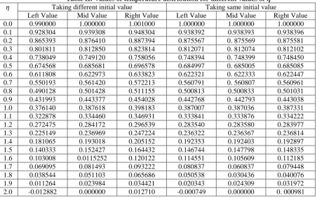
Table II: Values of temperature distribution for different values of Taking different initial value Taking same initial value

Left Value Mid Value Right Value Left Value Mid Value Right Value 0.0 0.990000 1.000000 1.001000 1.000000 1.000000 1.000000 0.1 0.928304 0.939308 0.948304 0.938392 0.938393 0.938396 0.2 0.865393 0.876410 0.887394 0.875567 0. 875569 0.875581 0.3 0.801811 0.812850 0.823814 0.812071 0. 812074 0.812102 0.4 0.738049 0.749120 0.758056 0.748394 0. 748399 0.748450 0.5 0.674568 0.685681 0.696578 0.684997 0. 685005 0.685085 0.6 0.611808 0.622973 0.633823 0.622321 0. 622333 0.622447 0.7 0.550193 0.561420 0.572213 0.560791 0. 560807 0.560961 0.8 0.490128 0.501428 0.511155 0.500813 0.500833 0.501031 0.9 0.431993 0.443377 0.454028 0.442768 0. 442793 0.443038 1.0 0.376140 0.387618 0.398183 0.387007 0.387036 0.387331 1.1 0.322878 0.334460 0.346931 0.333841 0.333876 0.334222 1.2 0.272475 0.284172 0.296539 0.283540 0.283580 0.283977 1.3 0.225149 0.236969 0.247224 0.236322 0.236367 0.236814 1.4 0.181065 0.193018 0.205152 0.192353 0.192403 0.192897 1.5 0.140333 0.152427 0.164432 0.146744 0.147798 0.148335 1.6 0.103008 0.0115252 0.120122 0.114551 0.105609 0.112185 1.7 0.069095 0.081493 0.093222 0.080837 0.060837 0.079448 1.8 0.038544 0.051103 0.065686 0.050538 0.030436 0.040076 1.9 0.011264 0.023984 0.034421 0.020343 0.024309 0.031972 2.0 -0.012882 0.000000 0.012710 -0.000749 0.000000 0. 000981

6. CONCLUSION

The initial right value, left value and the mid values are taken from the given boundary

conditions. As the velocity and temperature progresses from the initial point computations give the

(9)

IJSRR, 7(4) Oct. – Dec., 2018 Page 2464 So, from the above observations, we can conclude that the mid value of a triangular fuzzy number

coincides with the crisp value of the original problem.

7. REFERENCES

1. Sakiadis B C, AIChE J, 1961; 7: 26.

2. Crane L J, Z Angew Math Phys, 1970; 21: 645. 3. Wang C Y, Phys Fluids 1984; 27: 1915.

4. Troy W C, Overman E A X, Ermentrout H G B & Keener J P, Q Appl Math, 1987; 44:753. 5. Vajravelu K & Nayfeh J, ActaMech, 1993; 96: 47.

6. Mukhopadhyay S & Andersson H I, Heat Mass Transfer, 2009; 45:1447. 7. Jat R N & Chaudhury S, Z Angew Math Phys, 2010; 61: 1151.

8. Makinde O D & Aziz A, Int J Therm Sci, 2011; 50: 1326.

9. Mahapatra T R, Nandy S K, Vajravelu K & Gorder R A V, Mecanica, 2012; 47: 1623. 10.Chaudhury S, Chaudhury M K & Sharma R, Mechanica, 2015; 50: 1977.

11.Hiemenz K, Dingl Polytech J, 1911; 326: 321. 12.Homann F, Z Angew Math Mech, 1936; 16: 153.

13.Sparrow E M, Eckert E R & Minkowcz W J, ApplSci Res Sec A, 1962; 11:125. 14.Chiam T C, J Phys Soc Japan, 1994; 63: 2443.

15.Amin N & Riley N, J Fluid Mech, 1996; 314: 105.

16.Mahapatra T R & Gupta A S, Heat Mass Transfer, 2002; 38: 517. 17.Wang C Y, Int J Non-Lin Mech, 2008; 43: 377.

18.Rosali H, Ishak A & Pop I, Int Commun Heat Mass Transfer, 2011; 38: 1029. 19.Mahapatra T R & Nandy S K, Mechanica, 2013; 48: 23.

20.Lok Y Y & Pop I, Mechanica, 2014; 49: 1479.

21.Ingham D B & Pop I, Transport phenomena in porous media (Elsevier, U K), 1998. 22.Schlichting H & Gersten K, Boundary Layer Theory (Springer, Berlin), 2000. 23.Vafai K, Handbook of porous media- 2nd ed, (Taylor & Francis, New York), 2005. 24.Nield D A & Bejan A, Convection in porous media, 4th ed, (Springer, New York), 2012. 25.Vafai K & Kim S j, Int J Heat Fluid Flow, 1990; 11: 254.

26.Andersson H I, Acta Mech, 1992; 95: 227.

27.Mahapatra T R & Gupta A S, Acta Mech, 2001; 152: 191. 28.Abel M s & Mahesha N, Appl Math Model,2008; 32: 1965.

29.Ramesh G K, Gireesha B J & Bagewadi C S, Int J Heat Mass Tranfer, 2012; 55: 4900. 30.Singh R K & Singh A K, Appl Math Mech, 2012; 33 1207.

(10)

32.Olajuwon B I & Oahimire J I, Afrika Mathematika, 2014; 25: 911. 33.Chaudhury S & Kumar P, Indian J Pure Appl Phys, 2015; 53: 291.

34.de Barros L C, Bassanezi R C & Lodwick W A, A First Course in Fuzzy Logic, Fuzzy Dynamical Systems, and Biomathematics, (Springer), 2017.

35.Chakravarty S, Tapaswini S & Behera D, Fuzzy Arbitrary Order System Fuzzy Fractional Differential Equations and Applications, (Wiley), 2016.

36.Kaleva O, Fuzzy Sets and Systems, 1987; 24: 301.

37.Gomes L T, Barros L C de & Bede B, Fuzzy Differential Equations in Various Approaches, (Springer), 2015.

38.Kermani M A & Saburi F, Applied Mathematical Sciences, 2007; 1(27) : 1299.