www.nat-hazards-earth-syst-sci.net/10/773/2010/ © Author(s) 2010. This work is distributed under the Creative Commons Attribution 3.0 License.
Natural Hazards
and Earth
System Sciences
Abnormal storm waves in the winter East/Japan Sea:
generation process and hindcasting using an
atmosphere-wind wave modelling system
H. S. Lee1, K. O. Kim2, T. Yamashita1, T. Komaguchi3, and T. Mishima4
1Graduate School for International Development and Cooperation, Hiroshima University, Higashi-Hiroshima, Japan 2Korea Ocean Research & Development Institute, Ansan, Korea
3Blue Wave Institute of Technology Co., Ltd, Tokyo, Japan
4Blue Wave Institute of Technology Co., Ltd, Higashi-Hiroshima, Japan
Received: 3 August 2009 – Revised: 7 April 2010 – Accepted: 12 April 2010 – Published: 15 April 2010
Abstract. Abnormal storm waves cause coastal disasters
along the coasts of Korean Peninsula and Japan in the East/Japan Sea (EJS) in winter, arising due to developed low pressures during the East Asia winter monsoon. The gener-ation of these abnormal storm waves during rough sea states were studied and hindcast using an atmosphere-wave cou-pled modelling system. Wind waves and swell due to devel-oped low pressures were found to be the main components of abnormal storm waves. The meteorological conditions that generate these waves are classified into three patterns based on past literature that describes historical events as well as on numerical modelling. In hindcasting the abnormal storm waves, a bogussing scheme originally designed to simulate a tropical storm in a mesoscale meteorological model was in-troduced into the modelling system to enhance the resolution of developed low pressures. The modelling results with a bo-gussing scheme showed improvements in terms of resolved low pressure, surface wind field, and wave characteristics ob-tained with the wind field as an input.
1 Introduction
The surface winds over the East/Japan Sea (EJS) vary dis-tinctively with the seasons, blowing mild or moderate and variable in summer and very strong due to the East Asian monsoon and storms in winter. In winter atmospheric low pressures reacting with and passing through the EJS can sometimes cause abnormal storm waves on the Korean and Japanese coasts of the EJS.
Correspondence to: H. S. Lee (lee.hansoo@gmail.com)
In February 2008, abnormal storm waves due to a de-veloped atmospheric low pressure system propagating from the west off Hokkaido, Japan, to the south and southwest throughout the EJS caused extensive damage along the cen-tral coast of Japan on the EJS side and along the east coast of Korea. The accompanying high waves were mainly swells that developed with sufficient fetch over the EJS and lasted more than a day (Lee et al., 2008). The observed maximum wave heights and periods along the central coast of Japan are described in Table 1, while the observed maximum wave height and peak wave period at Anmok on the central east coast of Korea were 5.5 m and 14.17 s at 11:00:00 UTC on 24 February 2008. During February of that year, the abnor-mal storm waves at Toyama Bay, which are called “Yori-mawari Waves” in Japan, caused some of the most severe coastal damage ever induced by such conditions.
Many studies have examined the generation process and prediction of abnormal storm waves in the EJS. Some of the studies have been conducted in Japan, such as those described below. According to Kitaide (1952), the Yori-mawari Waves in Toyama Bay are long-period wind waves or swell generated due to the strong north and northeast-erly winds formed by a quasi-stationary developed atmo-spheric low-pressure area. Isozaki (1971) and Isozaki and Yoshio (1972) studied the characteristics of Yorimawari Waves and described their predictability based on meteo-rological observations and weather charts of past events. Yoshida et al. (1985) numerically studied an event of abnor-mal storm waves in the EJS using a simple spectral wave model based on an energy balance equation and showed that the wave heights were predictable to some extent, whereas the wave periods were not well coordinated with observa-tions. Yamaguchi et al. (1994) estimated extreme wave
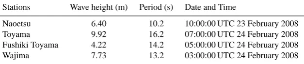
Table 1. Observed maximum values of wave characteristics in February 2008 (from Nationwide Ocean Wave information network for Port and HArbourS (NOWPHAS) of The Port and Airport Research Institute (PARI), Japan).
Stations Wave height (m) Period (s) Date and Time
Naoetsu 6.40 10.2 10:00:00 UTC 23 February 2008 Toyama 9.92 16.2 07:00:00 UTC 24 February 2008 Fushiki Toyama 4.22 14.2 05:00:00 UTC 24 February 2008 Wajima 7.73 13.2 03:00:00 UTC 24 February 2008
heights including Yorimawari Waves in the EJS by statisti-cal analysis of a number of wave hindcasting data obtained from spectral wave model simulations. In one study, Hatada and Yamaguchi (1998) suggested a method to predict the ab-normal storm waves quantitatively as they propagated toward the central coast of Japan in the EJS using a precise wave ray method and a shallow water prediction model. Recently, third-generation spectral wave models have been widely used to estimate wave characteristics not only in the EJS but in other seas as well.
In Korea, Choi and Joung (1979) studied abnormal storm waves that occurred in October 1976 using Wilson’s method of forcing by gradient wind and showed that the significant wave heights agreed fairly well with observations, while the corresponding wave periods needed to be improved. The wind field created by an extratropical cyclone was called a twister in their study. Joung et al. (1984) studied the gen-eration mechanism of a low-pressure system developed over the EJS on 2 January 1981 by analysing available data and using results from an adiabatic inviscid quasi-geostrophic model. To simulate meteorological conditions realistically, the authors considered required physical mechanisms such as a cold air outbreak, the topographical effects of the Ko-rean Peninsula, and a mesoscale convective complex. Jeong et al. (2007) studied abnormal storm waves of October 2006 based on wave and wind observations and found that the abnormal storm waves were a consequence of strong wind waves that propagated over swell to the east coast of Korea at the same time. Kim and Lee (2008) also studied the same abnormally high waves of October 2006 as well as those of October 2005 using a third-generation spectral wave model, SWAN, and showed that the results from numerical simula-tion were not satisfactory compared to observasimula-tions. One of the principal explanations proposed for their results was inac-curate wind forcing, imposed after linear interpolation of the simulation results from Regional Data Assimilation and Pre-diction System (RDAPS) of Korean Meteorological Agency (KMA).
Summarising the literature, abnormal storm waves in the EJS are mainly due to swells propagating from the west off Hokkaido caused by quasi-stationary developed atmospheric low pressures located to the east of or near Hokkaido, which can be categorised as an extratropical cyclone. When this
swell is propagated to the coasts around the EJS, either si-multaneously or consecutively accompanied by strong wind waves created by a tornado, abnormal storm waves are ob-served along the coasts and can cause damage or even disas-ter. The recent abnormal storm waves on 24 February 2008 and related coastal damage in Anmok, Korea, and in Toyama Bay, Japan, were typical of the phenomenon.
model and a third-generation spectral wave model. More-over, Yamashita et al. (2009) studied the possibility of more intense and frequent occurrence of extratropical cyclones in La Ni˜na (i.e., a forthcoming warm phase in terms of Pacific Decadal Oscillation) periods in the north-west Pacific, con-sidering climate change based on historical climate indices.
Since the abnormal storm waves are a key factor not only in coastal damage and disaster, but also in the design of coastal structures, it is critical to estimate these waves accu-rately, taking into account the meteorological conditions and topographical and bathymetric effects. Therefore, the objec-tives of this study are to improve wave field estimation using an atmosphere-wave coupled modelling system by introduc-ing a bogussintroduc-ing scheme to resolve the developed low pres-sure correctly and to study the generation mechanisms and characteristics of abnormal storm waves in the EJS in terms of meteorological conditions and numerical simulations.
This paper consists of six sections, as follows: In Sect. 2, the atmosphere-wave modelling system is described briefly. In Sect. 3, the bogussing scheme and its effects on meteo-rological modelling in the case of abnormal storm waves in December 2003 are described. The applications of the mod-elling system to two additional events, in February 1991 and February 2008, are described in Sect. 4. Discussions of the bogussing scheme and meteorological conditions for the ab-normal storm waves are presented in Sect. 5, which is fol-lowed by a summary and conclusions in Sect. 6.
2 Atmosphere-wave modelling system
2.1 Mesoscale meteorological model
The meteorological model in an atmosphere-wave modelling system is a three-dimensional non-hydrostatic mesoscale model, MM5, developed at Pennsylvania State University (PSU)-National Center for Atmospheric Research (NCAR). This model is based on non-hydrostatic, compressible form of governing equations in spherical and sigma coordinates with physical processes such as precipitation physics, Plane-tary Boundary Layer (PBL) processes and atmospheric radi-ation processes incorporated by a number of physics param-eterisations. MM5 also considers the complex topographical effects during the calculation. For more details on MM5, re-fer to Grell et al. (1995).
2.2 Wind wave model
The third generation wave model WaveWatchIII (WW3) was used in this study. The WW3 is based on the energy bal-ance equation and simulates wave propagation through geo-graphic, frequency and directional space. The wave refrac-tion, diffraction and shoaling due to spatial variances in wa-ter depth and currents are considered in WW3 simulation. Wave generation by wind input (Sin), energy dissipation by
whitecapping (Sds)and bottom friction (Sbot)and non-linear
wave-wave interactions (Snl)are taken into account in the
energy balance equation for source and sink terms. With the calculation of the energy balance equation in WW3, the two-dimensional directional spectrum,F (k,θ ), as well as the fur-ther action density spectrumN (k,θ )≡F (k,θ )/ω, can be ob-tained. Then, after integrating the two-dimensional spectrum over directions, an one-dimensional spectrum,F (k), can be generated, whereas total variation or wave energy,E, can be obtained by integrating over the whole spectrum. For more details of WW3 v2.22 used in this study, the interested reader is referred to Tolman (2002). The parameterisation of wave generation by wind input using the source term package by Tolman and Chalikov (1996) is described in the following paragraph. The frequency increment factor (Xω), first
fre-quency (ω0), number of frequencies and directions for all
simulations in the wave model were set to 1.1, 0.0412 Hz, 25 and 24, respectively.
How the energy is transferred from atmosphere to waves is of importance in an atmosphere-wave coupled modelling system. In WW3, the wind-wave interaction parameter,β, is introduced and approximated using the non-dimensional ap-parent wave frequency,ω˜aand drag coefficient,Cλ. The
sur-face drag coefficient and the actual wind input source term, Sin, to waves are a function of the two way interactions
be-tween atmosphere and waves and are calculated by iterative computation (Chalikov and Belevich, 1993; Chalikov, 1995).
3 Depression bogussing
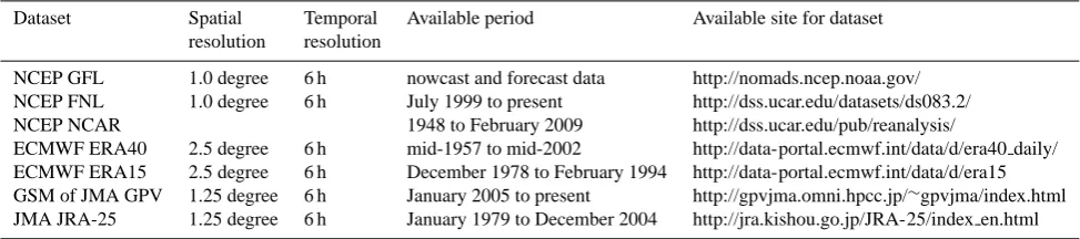
The available global meteorological data from atmospheric general circulation models (AGCMs) are used for short-term (hours or a few days), medium-range (up to 10 days), and seasonal forecasts and also for long-term climatic purposes. Depending on the range, AGCMs are coupled to different models for waves or ocean circulation. However, extreme weather events such as tropical cyclones, typhoons, hurri-canes and gales, as simulated by global AGCMs, are not ap-propriate for simulation of abnormal storm waves and ex-treme wave analysis. This is due to the coarse resolution of temporal and spatial dimensions in these models (see Ta-ble 2). For example, the global dataset of Japan Meteoro-logical Agency’s Grid Point Values (JMA GPV) shows only 60% to 70% of the magnitude of the observed wind speed (Fig. 5). Therefore, we introduced a bogussing scheme to improve our estimation of meteorological conditions such as wind and pressure field, which are the main driving forces of abnormal storm waves in the EJS, by resolving the developed low pressure more accurately in a mesoscale model. The bo-gussing scheme was first developed to improve the numerical simulation of tropical cyclones in a mesoscale model (Low-Nam and Davis, 2001); details are in Appendix A.
Table 2. Examples of freely available global meteorological dataset for background data of mesoscale model.
Dataset Spatial Temporal Available period Available site for dataset resolution resolution
NCEP GFL 1.0 degree 6 h nowcast and forecast data http://nomads.ncep.noaa.gov/ NCEP FNL 1.0 degree 6 h July 1999 to present http://dss.ucar.edu/datasets/ds083.2/ NCEP NCAR 1948 to February 2009 http://dss.ucar.edu/pub/reanalysis/
ECMWF ERA40 2.5 degree 6 h mid-1957 to mid-2002 http://data-portal.ecmwf.int/data/d/era40 daily/ ECMWF ERA15 2.5 degree 6 h December 1978 to February 1994 http://data-portal.ecmwf.int/data/d/era15 GSM of JMA GPV 1.25 degree 6 h January 2005 to present http://gpvjma.omni.hpcc.jp/∼gpvjma/index.html
JMA JRA-25 1.25 degree 6 h January 1979 to December 2004 http://jra.kishou.go.jp/JRA-25/index en.html
3.1 Effect of depression bogussing
As first guess, the bogussing scheme was performed on a wide range of grids in first guess to ensure that storms were completely removed from the background in the global model. If storms and vortices are not completely removed in the background data, the bogussing scheme generates a new storm or vortex wind over the background data. There-fore, there would be two or more storms and vortices in the initial state of the meteorological model run. For evaluation of the effect of a bogussing scheme on a low-pressure sys-tem, the method was applied to abnormal storm events in De-cember 2003, which had observed maximum wave heights of about 13 m at Naoetsu and caused coastal damage along the central coast of Japan on the EJS side.
For all applications in this study, high-resolution Black-adar PBL scheme (BlackBlack-adar, 1979), Reisner’s graupel mois-ture scheme (Reisner et al., 1998) and Grell cumulus scheme (Grell, 1993) were used because of the grid resolutions of 27 km for domain 1 and 9 km for domain 2. Four-dimensional data assimilation (FDDA) (Stauffer and Sea-man, 1990) was applied to the first and second domains in wind, temperature and mixing ratio fields. The other details of model configuration such as set-up of domains and initial and background data are described in their respective appli-cation subsections below.
3.2 Event in December 2003
3.2.1 Data
The meteorological conditions during the abnormal storm waves are shown in weather charts every twelve hours from 00:00:00 UTC 19 December to 12:00:00 UTC 20 Decem-ber 2003 (Fig. 1). An atmospheric low-pressure system with a minimum of 1000 hPa developed near Korean Peninsula was moving towards the east over the EJS at 00:00:00 UTC 19 December. Subsequently, this low-pressure system rapidly strengthened within a day in its central pressure from 1000 hPa to 972 hPa at 00:00:00 UTC 20 December while staying east off Aomori Prefecture for more than 12 h.
Dur-ing this movement, another atmospheric low-pressure system of 996 hPa was developing south of Hokkaido. This weaker low-pressure system also retained its strength for more than 12 h. During this development and the quasi-stationary states of two low-pressure zones, the winds were consistently blow-ing southward from the north and northeast. The observed winds at Ogata Wave Observatory (OWO) of Kyoto Univer-sity ranged from 18 to 22 m/s at 06:00:00 UTC 20 Decem-ber 2003 (Fig. 5a).
The bogussing scheme was applied to the two atmospheric low-pressure systems in Fig. 1, one with the lowest central pressure of 992 hPa, the maximum tangential wind (Vmax)
of 30 m/s, and the maximum radii (Rm) of 90 km located
in the EJS near the Aomori Prefecture, and the other with 972 hPa, 40 m/s, and 300 km located in the Pacific Ocean at 00:00:00 UTC 20 December 2003. These information of po-sitions and estimated maximum wind speeds and pressures were obtained from the JMA weather chart. The area of background data used for the bogussing scheme was in a 22×22 grids range of Global Spectral Model (GSM) data, because the search radius was fixed to 400 km and the radius of maximum wind speed was 90 km due to the resolution of GSM data. The Rankine vortex was used for wind profiles of the vortices.
Numerical simulations for this study had been conducted for conditions of abnormal storm waves observed at Naoetsu Harbour, Nigata Prefecture, Japan, at 07:00:00 UTC 20 De-cember in 2003. The recorded maximum and significant wave heights were 12.93 m and 9.24 m, respectively and the corresponding wave periods were 16.8 s and 12.9 s, respec-tively (Fig. 2). The abnormal high waves were also observed at OWO; however, the observed wave heights at OWO were limited and not credible because the water depth of measure-ment site at OWO was 7 m within a range of surf zone in rough sea.
3.2.2 Model set-up
H. S. Lee et al.: Abnormal storm waves in the winter East/Japan Sea 777
31
Figures
1 2
3
Fig. 1. Weather charts for 12 hour increments from 00:00 UTC 19 December to 12:00 UTC 20 December 2003 4
(from JMA). 5
6 7
(a) (b)
(c) (d)
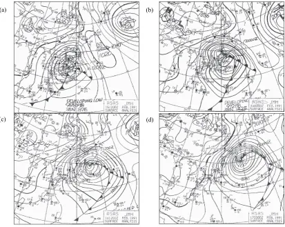
Fig. 1. Weather charts for 12 h increments from 00:00 UTC 19 December to 12:00 UTC 20 December 2003 (from JMA).
32 1
2
Fig. 2. Observed maximum wave height (○) and significant wave height (●) at Naoetsu and significant wave 3
height (+) from the Ogata Wave Observatory (OWO) of Kyoto University. 4
5
6
Fig. 2. Observed maximum wave height (◦) and significant wave height (•) at Naoetsu and significant wave height (+) from the Ogata Wave Observatory (OWO) of Kyoto University.
including both low-pressure systems (Fig. 3), whereas the domain D2 (with 9 km intervals) covers only the EJS and includes one of the developed lows located to the west of Aomori Prefecture. In addition, twenty-three vertical sigma layers from the surface up to 100 hPa level for both domains 2 and 3 plus 60×69 horizontal grids for domain 2 were set up for MM5 simulation with a 60 s time step. Computation of MM5 was carried out for six days from 00:00:00 UTC 17 to 00:00:00 UTC 23 December in 2003 with Real-time Global sea surface temperature (RTG SST) data (Gemmill et al., 2007).
Numerical simulations of wave model were performed for the two domains corresponding to those of MM5 with water depth taken from a general bathymetric chart of the oceans (Monahan, 2008) for domain 1 and 1 min regional digital bathymetry (Choi et al., 2002) for domain 2. The lateral and surface boundary conditions for the meteorological model were imposed every six hours from the GSM of JMA GPV dataset (Table 2). Three numerical computations were made under various conditions as shown in Table 3.
33 2
Fig. 3. Computational domains of the mesoscale model for the event of December 2003 and locations of OWO 3
of Kyoto University, Naoetsu Harbour, and P1 (at a point off Sado Island). 4
5 6
Fig. 3. Computational domains of the mesoscale model for the event of December 2003 and locations of OWO of Kyoto Univer-sity, Naoetsu Harbour, and P1 (a point off Sado Island).
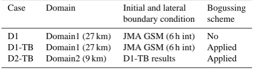
Table 3. Simulation conditions of WW3 for the event of December 2003.
Case Domain Initial and lateral Bogussing boundary condition scheme D1 Domain1 (27 km) JMA GSM (6 h int) No D1-TB Domain1 (27 km) JMA GSM (6 h int) Applied D2-TB Domain2 (9 km) D1-TB results Applied
3.2.3 Simulation results
Figure 4 shows the sea level pressure distribution of GSM data and simulation results of three simulation cases. The two atmospheric lows of GSM data were resolved, but some-what weaker than those in the JMA weather chart. The result of the D1 case did not show good resolution for the two lows, whereas with the bogussing scheme applied, the D1-TB and D2-TB cases yielded better results for sea level pressure dis-tribution, resolving the area of low pressure well.
The observed time-series data of wind speed at 10 m above sea surface at OWO and computed time-series data of three simulation cases at Naoetsu are compared in Fig. 5a. The observed and computed time-series data of significant wave
34 1
Fig. 4. Sea level pressure of (a) the operational GSM of the JMA GPV, (b) D1 case, (c) D1-TB case, and (d) 2
D2-TB case at 00:00 UTC 20 December 2003. 3
(a)
(b)
(c)
(d)
Fig. 4. Sea level pressure of (a) the operational GSM of the JMA GPV, (b) D1 case, (c) D1-TB case, and (d) D2-TB case at 00:00 UTC 20 December 2003.
H. S. Lee et al.: Abnormal storm waves in the winter East/Japan Sea 779
35 1
2
3
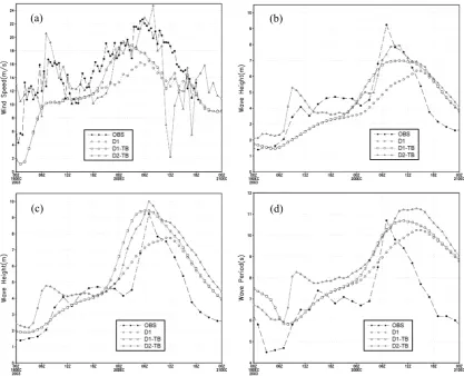
Fig. 5. Comparisons between observed and computed values from the abnormal storm wave event in December
4
2003. (a) Observed (propeller anemometer) U10 wind speed at OWO and computed (D1, D1-TB, D2-TB cases) 5
wind speed at Naoetsu, (b) observed (JMA) and computed (D1, D1-TB, D2-TB cases) significant wave heights 6
at Naoetsu, (c) observed (JMA) and computed (D1, D1-TB, D2-TB cases) significant wave heights at P1 (see 7
Fig. 4 for its position), and (d) observed (JMA) and computed (D1, D1-TB, D2-TB cases) significant wave 8
periods at Naoetsu. 9
10
11
(a) (b)
(c) (d)
Fig. 5. Comparisons between observed and computed values from the abnormal storm wave event in December 2003. (a) Observed (propeller anemometer)U10wind speed at OWO and computed (D1, D1-TB, D2-TB cases) wind speed at Naoetsu, (b) observed (JMA) and computed
(D1, D1-TB, D2-TB cases) significant wave heights at Naoetsu, (c) observed (JMA) and computed (D1, D1-TB, D2-TB cases) significant wave heights at P1 (see Fig. 4 for its location), and (d) observed (JMA) and computed (D1, D1-TB, D2-TB cases) significant wave periods at Naoetsu.
Fig. 4 are higher than the GSM data and D1 case, and they reproduce the changes of wind speed patterns as shown in Fig. 5a. The significant wave height at Naoetsu was some-what underestimated in all the cases. The best agreement among them is provided by the D2-TB case. In Fig. 5b and c, when compared to the other cases, the significant wave heights of the D1 case show a time delay of about six hours. The simulation results of the D1 case using GSM data in Fig. 5b to d show that neither the reproduction of the wind fields nor the hindcasting of abnormal storm waves using the modelled wind data were accurate. This is primarily due to the coarse spatial and temporal resolution of the global back-ground data.
4 Hindcasts of abnormal storm waves
Two additional simulations of abnormal storm waves, in February 1991 and February 2008, were performed to inves-tigate the generation process and the characteristics of abnor-mal storm waves in the EJS. The two events caused coastal damage along the east coast of Korea and the central coast of Japan in the EJS. These two events were selected because the abnormal storm waves in February 2008 caused some of the most severe coastal damage ever recorded, and fairly good observations were made during the event, whereas the waves in February 1991 caused less coastal damage, al-though higher values of wave characteristics were observed than in the 2008 event. The observed data, model configu-ration and the results are described in the following subsec-tions.
36
2
Fig. 6. Weather charts for twelve hour increments from 12:00 UTC 15 February to 00:00 UTC 17 February 1991 3
(from JMA). 4
5
6
(a) (b)
(c) (d)
Fig. 6. Weather charts for twelve hour increments from 12:00 UTC 15 February to 00:00 UTC 17 February 1991 (from JMA).
4.1 Event in February 1991
4.1.1 Data
The meteorological conditions during the abnormal storm waves in February 1991 are presented in Fig. 6. An area of low pressure was well developed to the west of Kyushu, Japan, in the East China Sea at 00:00:00 UTC 14 Febru-ary 1991 and moved slowly eastward. While the low pres-sure area was moving eastward, another low-prespres-sure system developed very nearby, and the two systems strengthened, with a central pressure dropping to 990 hPa and 988 hPa, re-spectively, at 12:00:00 UTC 15 February 1991. Then the two pressure systems merged into one developed low-pressure system while moving northeast over Honshu, Japan. When the low-pressure system approached the area east of Aomori, it kept its quasi-stationary state and strengthened continuously as its central pressure dropped to 960 hPa at 00:00:00 UTC 17 February 1991.
4.1.2 Model set-up
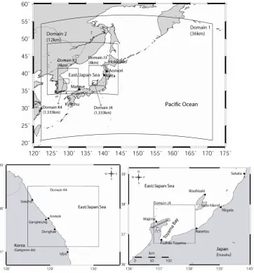
Figure 7 shows the computational domains for the meteo-rological and wave models. A four-level nesting was per-formed throughout the simulations with grid intervals of 36 km, 12 km, 4 km, and 1.333 km for each domain both in atmosphere and in wave modelling. The largest domain cov-ers the entire Korean Peninsula, Japan, the EJS, and parts of the north-west Pacific Ocean, allowing correct simulation of the large-scale meteorological features while reducing the boundary effects on the focus area.
37 1
2 3
4 5
Fig. 7. Computational domains of meteorological and wave models for the events of February 1991 and
6
February 2008 and locations of wave and weather observation stations along the coasts of Korea and Japan. In 7
the event of February 1991, only the domains 1, 2, J3 and J4 were used while all domains including K3 and K4 8
were used for the event of February 2008. 9
10
11
Fig. 7. Computational domains of meteorological and wave models for the events of February 1991 and February 2008 and locations of wave and weather observation stations along the coasts of Korea and Japan. In the event of February 1991, only the domains 1, 2, J3 and J4 were used while all domains including K3 and K4 were used for the event of February 2008.
The water depths for wave modelling were taken from a general bathymetric chart of the oceans (Monahan, 2008) for domain 1, 1 min regional digital bathymetry (Choi et al., 2002) for domain 2 and Japan Oceanographic Data Center (JODC) bathymetry for domains 3 and 4.
4.1.3 Simulation results
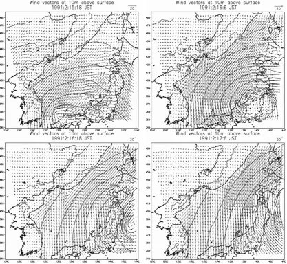
The calculated wind fields using the JRA-25 dataset for initial and boundary conditions every twelve hours from 09:00:00 UTC 15 February to 21:00:00 UTC 16 Febru-ary 1991 are shown in Fig. 8. The low pressure generated off west Kyushu was located west of Honshu, Japan, and was moving to the northeast at 09:00:00 UTC 15 February 1991. The low pressure continued to move northeast and was po-sitioned east of Aomori with strong winds over the EJS at 09:00:00 UTC 16 February 1991, as shown in Fig. 8. While
the developed low pressure maintained a quasi-stationary state east of Aomori, starting from noon of 16 February the strong winds of about 20 m/s in the north and northeast direc-tion continued for more than a day. These wind field results agreed well with the weather charts during the simulations.
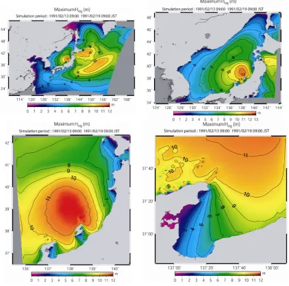
The spatial distributions of calculated maximum signifi-cant wave heights using the JRA-25 dataset for initial and boundary conditions are presented during the simulation pe-riod from all domains in Fig. 9. The growth of surface waves in the EJS is rather limited since it is a semi-enclosed water mass; this is indicated in the results from domains 1 and 2. The contour of 5 m significant wave height extended to the east coast of Korea. The barrier effect of Sado Island and the bathymetric effects at Toyama Bay can also be seen in the spatial distributions of significant wave heights of domains 3 and 4.
38 1
2 3
Fig. 8. Calculated wind vectors and isobars from domain 2 for twelve 12 hour increments from 09:00 UTC 15 4
February to 21:00 UTC 16 February 1991 using JRA-25 for initial and boundary conditions of MM5. 5
6 7
Fig. 8. Calculated wind vectors and isobars from domain 2 for twelve hour increments from 09:00 UTC 15 February to 21:00 UTC 16 Febru-ary 1991 using JRA-25 for initial and boundFebru-ary conditions of MM5.
Calculated significant wave heights and periods using the ERA40, JRA-25, and NCEP NCAR datasets at Fushiki Toyama, Naoetsu, Wajima, and Sakata are presented at Fig. 10. The calculated results at Wajima and Sakata only are compared with the available observations. From all loca-tions, the results using the ERA40 dataset showed the largest values for significant wave periods with sharp increase, while the results using the JRA-25 dataset depicted rather small values for wave periods with mild gradients. The results with the JRA-25 dataset also show the smallest values for signif-icant wave heights at all locations. At Wajima and Sakata, the results in wave periods using the JRA-25 dataset showed better agreement with the observations than the other results. In significant wave heights, the results with JRA-25 showed better agreement with the observations than the other results at Sakata, while those at Wajima were somewhat underesti-mated during the peak of observed significant wave heights
from 04:00:00 UTC 16 to 04:00:00 UTC 17 February 1991 compared to the observations.
4.2 Event in February 2008
4.2.1 Data
39 1
2 3
Fig. 9. Distribution of calculated maximum significant wave heights for domain 1, 2, 3, and 4 for the event of 4
February 1991 using JRA-25 for initial and boundary conditions of MM5. 5
6 7
Fig. 9. Distribution of calculated maximum significant wave heights for domain 1, 2, 3, and 4 for the event of February 1991 using JRA-25 for initial and boundary conditions of MM5.
further. Another low-pressure system also developed south-east of Honshu and moved northsouth-eastward until it neared the other low-pressure system. Due to these meteorologi-cal conditions, westerly and northwesterly winds were dom-inant during the slow movement of low pressure over the EJS on 22 February while strong north and northeasterly winds of around 20 m/s were blowing dominantly on 23 and 24 February. The observed winds from JMA Auto-mated Meteorological Data Acquisition System (AMEDAS) at Washizaki, Sado Island, were 18 m/s in a northwest direc-tion at 13:30:00 UTC 23 February and 20 m/s in the same di-rection at 20:40:00 UTC 23 February. The observed wind at Fushiki, Toyama, was 7.6 m/s in the northwest direction and 6 m/s in the north direction at 12:00:00 UTC 23 February and at 09:00:00 UTC 24 February, respectively. Therefore, we
determined that the high waves that caused the coastal dam-age in Toyama Bay were not under the influence of strong winds.
The observed wave characteristics are presented in Ta-ble 1. The maximum values of wave height and period at Naoetsu were observed at 10:00:00 UTC 23 February, whereas those at Toyama, Fushiki Toyama, and Wajima were observed in the afternoon on 24 February. Moreover, the observed maximum value of wave period at Naoetsu was smaller than the others. From the meteorological condi-tions and wave observacondi-tions, it can be determined that the peak values of the wave characteristics at Naoetsu were due to high waves caused by the slowly moving low pressure through the EJS, while the values at the other locations were due to the swell caused by the quasi-stationary low-pressure
40 1
2
3
4 5
Fig. 10. Comparisons of observations and calculations of wave characteristics at Fushiki Toyama, Naoetsu,
6
Wajima, and Sakata in Japan for the event of February 1991. The observations were available only from Wajima 7
and Sakata. 8
9
Fig. 10. Comparisons of observations and calculations of wave characteristics at Fushiki Toyama, Naoetsu, Wajima, and Sakata in Japan for the event of February 1991. The observations were avail-able only from Wajima and Sakata.
systems east of Hokkaido. Sado Island also played a role as a barrier against the swell that was propagating towards Naoetsu. The observed maximum values of wave height and wave period at Anmok in the central east coast of Korea were 5.5 m and 14.17 s at 11:00:00 UTC 24 February 2008. These waves were also due to the swell caused by the quasi-stationary low-pressure systems.
4.2.2 Model set-up
Figure 7 shows the computational domains for the mete-orological and wave models. Four level nesting was per-formed throughout the simulations with grid intervals of 36 km, 12 km, 4 km, and 1.333 km for each domain. The domains 1, 2, J3 and J4 were the same as the domains used in the simulation for February 1991, with domains 1 and 2 covering the EJS and parts of the northwest Pacific Ocean. In this case, two more domains were added to the case of 1991 to cover the east coast of Korea including Anmok, Gangwon-do (Fig. 7), where abnormal storm waves were ob-served. The simulation was carried out over a period of 78 h from 00:00:00 UTC 22 February to 06:00:00 UTC 25 Febru-ary 2008. The initial condition and lateral and surface bound-ary conditions for the meteorological model were imposed every six hours from NCEP FNL (Final) Operational Global Analysis data (Table 2). FDDA was also applied to the first domain in wind, temperature and mixing ratio fields every six hours with NCEP FNL data. The water depths of wave modelling for domains 1, 2, J3, and J4 were the same as those of the 1991 case, while the water depths for domain K3 and K4 were taken from the 1 min regional digital bathymetry (Choi et al., 2002).
4.2.3 Simulation results
The calculated wind vectors from domain 2 were recorded every six hours from 21:00:00 UTC 22 February to 15:00:00 UTC 23 February 2008 are shown in Fig. 12. Coun-terclockwise wind vectors are clearly presented in the figure at 21:00:00 UTC 22 and 03:00:00 UTC 23 February as the low-pressure area moved eastward. The winds strengthened as the low pressure neared Aomori and joined the other de-veloped low pressure. After the low pressure passed over the EJS, the strong north and northwesterly winds were pre-dominant; these calculated wind patterns agree well with the weather charts in Fig. 11. The calculated wind speeds and directions were compared with observations at Matsue, Ni-igata, Sakata, and Akita from JMA AMEDAS (see Fig. 7 for their locations). These four stations are located along the Japanese coast on the EJS side. The calculated wind speeds and directions showed good accordance with the observa-tions, while the estimated wind speed at Niigata was a bit higher than the observation (see Fig. 13).
The results in Fig. 14 are similar to those shown in Fig. 9 in terms of characteristics of surface wave growth in the EJS from domains 1 and 2 and the barrier effect of Sado Island and the bathymetric effects at Toyama Bay from domains 3 and 4.
41 1
2
Fig. 11. Weather charts for twelve hour increments from 12:00 UTC 22 February to 00:00 UTC 24 February 3
2008 (from JMA). 4
5
6
(a) (b)
(c) (d)
Fig. 11. Weather charts for twelve hour increments from 12:00 UTC 22 February to 00:00 UTC 24 February 2008 (from JMA).
were under the influence of developed wind waves from the west or northwest direction due to the moving low pressure and swell from the north and northeast due to the sequen-tial quasi-stationary low-pressure systems occurring from around noontime on 23 February. The Fushiki Toyama sta-tion was affected only by the swell propagated from north and northeast direction due to the Noto Peninsula (Fig. 7).
The simulation results at Anmok, Korea, show good agree-ment with observations of significant wave height, as shown in Fig. 16. However, the corresponding wave period was somewhat underestimated in the simulation. Due to the movement of the low-pressure area eastward from the Ko-rean Peninsula, Anmok station was under the influence of developed wind waves beginning early in the morning on 23 February, and these high waves continued for more than two days due to the ensuing swell after the developed wind waves.
In Figs. 17 and 18, the two-dimensional wave spectra at Fushiki Toyama and Anmok are presented for 6-h and 12-h periods respectively during the simulation. Wave energy has a wide range of frequencies and directions, whereas swell
en-ergy is distributed over a narrow range of frequencies and di-rections. It is important to note that wave direction is shown in terms of propagating away from the grid point; in other words, it propagates toward the edge of the plot, following the oceanographic convention, which is contrary to the at-mospheric convention for wind direction.
In Fig. 17, at 05:00:00 UTC 23 February, the relatively young wind waves with a period of 4 to 5 s dominate due to the slow-moving low pressure from the north to northeast direction. Then a relatively young swell appeared that was moving in the north-east-north direction at 11:00:00 UTC 23 February, but the wind waves were still dominant in wave energy. Six hours later, the swell was more developed and became dominant, but still the wind waves coexisted with the swell at 17:00:00 UTC 23 February. The double-peaked frequency spectrum in the northeast direction became a one-peak spectrum with a dominant swell in the northeast at 23:00:00 UTC 23 February, and the energy of wind waves disappeared. Subsequently, the wave energy in a narrow fre-quency band in the northeast direction caused by the devel-oped swell from the quasi-stationary low-pressure systems
42 2
Fig. 12. Calculated wind vectors and isobars from domain 2 for six hour increments from 21:00 UTC 22 3
February to 15:00 UTC 23 February 2008. 4
5
6
Fig. 12. Calculated wind vectors and isobars from domain 2 for six hour increments from 21:00 UTC 22 February to 15:00 UTC 23 Febru-ary 2008.
occupied the spectral plots, even though the winds became weak in a different direction from 07:00:00 UTC 24 Febru-ary at Fushiki Toyama, as shown in Fig. 17.
At Anmok, Korea, the wave energy group in the top right at 21:00:00 UTC 22 February due to wind waves caused by moving the dominating low pressure, and the dominant pe-riod was about 7 to 8 s. Then the wind waves became more developed with a dominant period of around 10 s, showing the wave energy in a wide range of frequency and direc-tion until 21:00:00 UTC 23 February. The dominant wave energy, then, became narrow in frequency at 09:00:00 UTC 24 February due to the incoming swell, even though the wave energy still varied in direction due to the open location of a wave measurement instrument at Anmok. When the local wind was very weak, the high wave energy due to the swell existed in the northeast direction, showing that the dominant wave energy became narrow in both frequency and
direc-tion at 21:00:00 UTC 24 February. Because the wave peri-ods were somewhat underestimated in simulation at Anmok, the frequency spectrum from observed data is expected to be more centre-biased than the calculated one.
5 Discussion
Since the main reason for abnormal storm waves in the EJS is the wind field input due to low pressures in winter, we classified three patterns of meteorological conditions for the generation process based on the literature reviews mentioned in Sect. 1, which dealt with various events of abnormal storm waves in the EJS and the numerical simulations performed in this study.
43 1
2
3
4 5
Fig. 13. Comparisons of observations and calculations of winds at Matsue, Niigata, Sakata and Akita in Japan 6
for the event of February 2008. 7
8
Fig. 13. Comparisons of observations and calculations of winds at Matsue, Niigata, Sakata and Akita in Japan for the event of Febru-ary 2008.
becomes a quasi-stationary low-pressure system east of or near Hokkaido, Japan. Under this condition, the wind waves caused by the moving low pressure are followed by the swell resulting from the quasi-stationary state of the low pressure. The abnormal storm waves in December 2003 and Febru-ary 2008 were examples of this pattern.
Second, an area of low pressure develops in East China Sea or south of Honshu, the main island of Japan, moves northeast or north to near Hokkaido, and then becomes a quasi-stationary low-pressure system causing the swell in the EJS. The abnormal storm waves in February 1991 were an example of this second pattern.
Third, a low-pressure system generated over the continent of East Asia or near the Korean Peninsula moves southeast-ward over the EJS and the Japanese islands or becomes weak and disappears in the EJS. The abnormal storm waves in Oc-tober 2006 were in this third category (see Fig. 19 for meteo-rological conditions of a slowly moving low pressure toward the southeast). In this kind of meteorological pattern, the east coast of Korea is under the strong influence of wind waves. Kim and Lee (2008) reported details of the event in Octo-ber 2006.
In any of the conditions above, it is important to note that there was another second low-pressure system that was gen-erated and developed in the Pacific Ocean. This second pressure system caused the quasi-stationary state of the low-pressure system from the EJS by somehow blocking east-ward movement as a part of the wintertime meteorological conditions over East Asia and the northwest Pacific. There-fore, it is desirable to consider all these meteorological con-ditions in meteorological modelling to account for the exter-nal forces on surface waves in wave modelling. The moving speed of low-pressure systems and the sea surface temper-ature are also important factors that decide the intensity of wind fields caused by low pressure, similar to storm waves created by tropical cyclones. Table 4 shows the classifica-tion of past events based on the above three patterns of me-teorological conditions. The term “Unknown” in the pattern column indicates that no data is available to determine the pattern, while the mark,∗, indicate a guess based on avail-able data in Tavail-able 4.
Although the bogussing scheme is a very effective method to resolve and describe the developed low-pressure systems in this study, care should be taken when applying it to a low-pressure system. Because the horizontal wind profile in the bogussing scheme is produced by the Rankine vortex, the radii of maximum wind (Rm)and maximum wind speed
(Vmax) are essential information to include on the vortex
wind profile (see Eq. A2). However, theRmis not normally
available even for low-pressure systems on weather charts. Therefore, this information is assumed based on available information of tropical storms of a similar scale. Moreover, due to the grid intervals of the computational domains of the meteorological model, theRm is inevitably pre-determined.
Hence, it is difficult to apply these data in wave forecasting.
6 Summary and conclusions
In this study we described the results of long-term continu-ous researches on the abnormal storm waves caused by de-veloped low pressures evolving and moving over the EJS in winter. It focuses on the generation process and hind-cast based on literature review and numerical modelling us-ing an atmosphere-wave modellus-ing system. The simulations were performed for three recorded events of abnormal storm waves in the order of the events in 2003, 1991 and 2008. In
44 1
2 3
Fig. 14. Distribution of calculated maximum significant wave heights for domains 1, 2, 3, and 4 for the event of
4
February 2008. 5
6
7
Fig. 14. Distribution of calculated maximum significant wave heights for domains 1, 2, 3, and 4 for the event of February 2008.
Table 4. Classification of past events in terms of meteorological conditions.
Date Patterns based on the Related coastal damages Reference track of low pressure
2 January 1929 Pattern 2 Toyama Bay, Japan Kitaide (1952) 9 December 1943 Pattern 1 Toyama Bay, Japan Kitaide (1952) 16 February 1949 Pattern 2 Toyama Bay, Japan Kitaide (1952) 6 January 1963 Pattern 1∗ Toyama Bay, Japan Isozaki and Yoshio (1972)
31 December 1965 Unknown Toyama Bay, Japan Isozaki and Yoshio (1972) 23 February 1966 Pattern 2 Toyama Bay, Japan Isozaki (1971) 28 October 1967 Pattern 2 (Typhoon) Toyama Bay, Japan Isozaki and Yoshio (1972) 31 January 1970 Pattern 2 Toyama Bay, Japan Isozaki and Yoshio (1972) 28 December 1976 Pattern 2 Toyama Bay, Japan Hatada and Yamaguchi (1998) 26 October 1976 Pattern 1 Dae Wha Bank in the EJS Choi and Joung (1979)
2 January 1981 Pattern 1 Joung et al. (1984)
16 January 1984 Unknown Toyama Bay, Japan Yoshida et al. (1985) 16 February 1991 Pattern 2 Toyama Bay, Japan This study 20 December 2003 Pattern 1 Toyama Bay, Japan This study 23 October 2005 Pattern 1 East coast of Korea Kim and Lee (2008)
12 October 2006 Pattern 3 East coast of Korea Jeong et al. (2007) and Kim and Lee (2008) 23 February 2008 Pattern 1 Anmok, Korean and Toayama Bay, Japan Lee et al. (2008)
45 1
2
3
4 5
Fig. 15. Comparisons of observations and calculations of wave characteristics at Wajima, Sakata, Naoetsu and 6
Fushiki Toyama in Japan for the event of February 2008. 7
Fig. 15. Comparisons of observations and calculations of wave characteristics at Wajima, Sakata, Naoetsu and Fushiki Toyama in Japan for the event of February 2008.
the case of 2003 event, one of the objectives of the study was to evaluate the applicability of bogussing scheme to extra-tropical cyclones with available GSM data in addition to the investigation of the generation process of abnormal storm waves. In the case of 1991, the objective was to compare the freely available dataset (ECMWF ERA40, NCEP NCAR data, and JMA JRA-25) for wave modelling in addition to the original purpose. NCEP FNL dataset is not available for the year of 1991. In the case of 2008, the NCEP FNL dataset was chosen for the simulation of the abnormal storm waves.
46 1
2
Fig. 16. Comparisons of observations and calculations of wave characteristics at Anmok in Korea for the event 3
of February 2008. 4
5
6
Fig. 16. Comparisons of observations and calculations of wave characteristics at Anmok in Korea for the event of February 2008.
The performance of the numerical simulations of a mete-orological model when using a bogussing scheme was im-proved for both the resolved low-pressure system and sur-face wind field (U10)in the events of December 2003 with
respect to those from the GSM of JMA GPV and the model run without a bogussing scheme. The abnormal storm waves recorded at Naoetsu Harbour and OWO on 20 December in 2003 were reproduced by the modelling system, deriving simulation results that were close to the observed values of a significant wave height of 9.24 m and significant wave period of 12.9 s.
In addition to the bogussing scheme to improve meteoro-logical modelling, three kinds of available global datasets, ERA40, JRA-25, and NCEP NCAR, were used for back-ground data of the meteorological model to investigate the characteristics and effect of the grid resolution of the dataset. In comparison with available wave observations at Wajima and Sakata, Japan, the results with JRA-25 showed closer agreement with observations. The grid resolution of JRA-25 (1.25 deg) may be the main reason for the results, since the horizontal wind profile by the bogussing scheme is some-what pre-determined by the grid resolution of background data and computational domains. In the case of the Febru-ary 2008 event, the calculated wind and wave field were com-pared with observations and showed good agreement. The swell components in surface waves were clearly identified from wave spectral plots at Anmok and Fushiki Toyama.
The meteorological conditions that cause abnormal storm waves in the EJS are classified into three patterns based on the literature of historical events and numerical modelling. The speed and track of a low-pressure system and the in-teraction with another pressure system in the East Asia and north Pacific regions are the main factors in the classifica-tion, although some important physical parameters are not considered in this study.
In air-sea interaction, the transfer of heat, mass and mo-mentum between air and sea depends on conditions such as sea surface temperature, the temperature difference be-tween air and underlying sea, and wind waves. In particular, the wind waves are considered the most important factor in
47 1
2 3
Fig. 17. Calculated 2-D wave spectral plots at Fushiki Toyama, Japan, for the event of February 2008. Time and 4
significant wave height are shown above each panel, while wind speed and direction are shown below and in the 5
centre of each panel, respectively. The 16-level shaded colours represent wave energy density (m2/Hz) being
6
doubled in each level, with dark blue indicating the absence of wave energy (1.61238e-04) and light purple 7
indicating a local maximum (10.56695). Wave direction is toward the edge of the plot. 8
Fig. 17. Calculated 2-D wave spectral plots at Fushiki Toyama, Japan, for the event of February 2008. Time and significant wave height are shown above each panel, while wind speed and direction are shown below and in the centre of each panel, respectively. The 16-level shaded colours represent wave energy density (m2/Hz) be-ing doubled in each level, with dark blue indicatbe-ing the absence of wave energy (1.61238e-04) and light purple indicating a local max-imum (10.56695). Wave direction is toward the edge of the plot.
understanding air-sea interaction. Although air-sea interac-tion has been a subject of discussion for a long time, the most useful observations covering all wind regimes from weak and mild to very strong ones under tropical cyclones have only recently become available (Edson et al., 2007). In a low-wind regime, turbulence and turbulent mixing have low in-tensity in the marine atmospheric boundary layer. The sur-face wave modulation is clearly observable in wind veloci-ties, static pressure and humidity. In moderate winds, turbu-lence has the dominant influence on water vapour and flow velocities, while the pressure field is organised and coher-ent with the waves (Hristov, 2005). In high winds such as
48 1
2
Fig. 18. Calculated 2-D wave spectral plots Anmok, Korea, for the event of February 2008. Time and significant 3
wave height are shown above each panel, while wind speed and direction are shown below and in the centre of 4
each panel, respectively. The 16-level shaded colours represent wave energy density (m2/Hz) being doubled in
5
each level, with dark blue indicating the absence of wave energy (1.61238e-04) and light purple indicating a 6
local maximum (10.56695). Wave direction is toward the edge of the plot. 7
8
Fig. 18. As in Fig. 17, but at Anmok, Korea.
in tropical cyclones, the interaction processes are influenced by sea spray, spume and air flow separation due to break-ing of surface waves (Doyle, 2002). The effect of waves on ocean surface currents and the ocean mixed layer is also a complex phenomenon in air-sea interaction. These effects of surface waves on the marine atmospheric boundary layer, however, are not considered in the atmosphere-wave coupled modelling system in this study and remain a subject and a guide for further study.
49 1
2
Fig. 19. Weather charts at 00:00 UTC 22, at 12:00 UTC 22, at 06:00 UTC 23 and at 00:00 UTC 24 October 2006 3
(from JMA). 4
5
(a) (b)
(c) (d)
Fig. 19. Weather charts at 00:00 UTC 22, at 12:00 UTC 22, at 06:00 UTC 23 and at 00:00 UTC 24 October 2006 (from JMA).
Appendix A
The bogussing scheme is performed in two steps in the RE-GRID process of MM5 as follows.
A1 Detection and removal of cyclones
1. Searching for the storm centre in first guess within the searching radius (fixed to 400 km) according to the given Best Track position.
2. Removal of first guess vortices and divergence within 300 km of first guess storm and recomputed velocity. 3. Removal of geostrophic vortices within 300 km of first
guess storm and associated geopotential heights. 4. Removal of the temperature anomaly from the
hydro-static relation using calculated geopotential anomaly. 5. Removal of enhanced relative humidity within 600 km
of first guess storm.
6. Specifying bogus storm velocity and stream function centred on Best Track position.
7. Solving of the non-linear balance equation for geopo-tential heights.
8. Calculation of the bogus temperature from the balanced height field.
9. Modification of relative humidity to be nearly saturated out to a radius of maximum wind (Rm)and mixing it
with the background at 1200 km radius.
A2 Generation and blending with modified first guess
The bogus vortex wind profile was generated using the Rank-ine vortex model below based on several assumptions,
v=A(z)F (r) (A1)
F (r)=
Vmax
Rm r if r≤Rm Vmax
Rα
m r
α if r > R m
(A2)
whereα= −0.75 is a parameter for wind profiles at large radii (r > Rm),Rmis the maximum radius, andVmaxis the
maximum tangential wind speed. The assumptions are given as follows:
1. axi-symmetry
2. fixed radius of maximum wind field (discussed in detail in Sect. 5)
3. nearly saturated bogus vortex field 4. mass and wind field in nonlinear balance
5. maximum bogus winds as a pre-determined fraction of maximum winds provided
Because insufficient data are available on asymmetry for tropical cyclones, the bogus vortex is assumed to be axi-symmetric; therefore, the simulated maximum wind speed is somewhat lower than the observed maximum wind speed. A new bogus vortex or modified wind profile with respect to the asymmetry of real tropical storms is needed to improve the horizontal wind profile.
Acknowledgements. We thank the anonymous reviewers, whose
comments helped us improve the quality of this paper. This study was supported by the Global Environment Leader Education Program for Designing a Low-Carbon Society under the auspices of MEXT Special Coordination Funds for Promotion of Science and Technology in the Graduate School for International Development and Cooperation, Hiroshima University. The second author was supported by Korea Ocean Research & Development Institute (PE9842H) and Korea Institute of Marine Science & Technology Promotion (PM55210).
Edited by: A. Mugnai
Reviewed by: three anonymous referees
References
Blackadar, A. K.: High-resolution models of the planetary bound-ary layer, in: Adv. Environ. Sci. Eng., edited by: Pfafflin, I. J. R. and Ziegler, E. N., 1, Gordon and Breach Science Publishers, 50–85, 1979.
Cavaleri, L. and Bertotti, L.: Accuracy of the modelled wind and wave fields in enclosed seas, Tellus A, 56, 167–175, 2004. Cavaleri, L. and Bertotti, L.: The improvement of modelled wind
and wave fields with increasing resolution, Ocean Eng., 33, 553– 565, 2006.
Chalikov, D.: The parameterization of the wave boundary layer, J. Phys. Oceanogr., 25, 1333–1349, 1995.
Chalikov, D. V. and Belevich, M. Y.: One-dimensional theory of the wave boundary layer, Bound.-Lay. Meteorol., 63, 65–96, 1993. Choi, B. H., Kim, K. O., and Eum, H. M.: Digital bathymetric
and topographic data for neighboring seas of Korea (in Korean with English abstract), J. Korean Society of Coastal and Ocean Engineers, 14, 41–50, 2002.
Choi, H. and Joung, C. H.: A study on the numerical calculation for wind waves generated by extratropical cyclones developed rapidly in the Sea of Japan (in Korean with English abstract), J. Korean Met. Soc., 15, 35–43, 1979.
Doyle, J. D.: Coupled Atmosphere-Ocean Wave Simulations under High Wind Conditions, Mon. Wea. Rev., 130, 3087–3099, 2002. Edson, J., Crawford, T., Crescenti, J., Farrar, T., Frew, N., Gerbi, G., Helmis, C., Hristov, T., Khelif, D., Jessup, A., Jonsson, H., Li, M., Mahrt, L., McGillis, W., Plueddemann, A., Shen, L., Skyllingstad, E., Stanton, T., Sullivan, P., Sun, J., Trowbridge, J., Vickers, D., Wang, S., Wang, Q., Weller, R., Wilkin, J., Williams, A. J., Yue, D. K. P., and Zappa, C.: The Coupled Boundary Lay-ers and Air-Sea Transfer Experiment in Low Winds, B. Am. Me-teorol. Soc. , 88, 341–356, 2007.
Gemmill, W., Katz, B., and Li, X.: Daily Real-Time Global Sea Sur-face Temperature – High Resolution Analysis at NOAA/NCEP, NOAA/NWS/NCEP/MMAB Office Note Nr. 260, 39, 2007. Grell, G. A.: Prognostic Evaluation of Assumptions Used by
Cu-mulus Parameterizations, Mon. Wea. Rev., 121, 764–787, 1993. Grell, G. A., Dudhia, J., and Stauffer, D. R.: A description of
the fifth-generation Penn State/NCAR Mesoscale Model (MM5), National Center for Atmospheric Research, NCAR Tech. Note, NCAR/TN-398 + STR, 1995.
Hatada, Y. and Yamaguchi, M.: Preliminary study on a prediction method of large swell-like waves in Toyama Bay ‘Yorimawari-Nami’ , Memoirs of the Faculty of Eng., Ehime Univ., 17, 261– 271, 1998 (in Japanese with English abstract).
Hristov, T.: Wave-driven scalar ?elds in marine atmospheric bound-ary layer, Geophys. Res. Abstr., 7, 02863, 2005.
Isozaki, I.: On the characteristics of coastal waves on the coast of Toyama Bay (Report I) (in Japanese with English abstract), Notes of Cooperative Research for Disaster Prevention, 25, 3– 15, 1971.
Isozaki, I. and Yoshio, O.: On the characteristics of coastal waves on the coast of Toyama Bay (Report II), Notes of Cooperative Research for Disaster Prevention, 28, 3–17, 1972 (in Japanese with English abstract).
Jeong, W. M., Oh, S.-H., and Lee, D. Y.: Abnormally high waves on the East Coast, J. Korean Society of Coastal and Ocean Engi-neers, 19, 295–302, 2007 (in Korean with English abstract).
Joung, C.-H., Kim, S. S., Park, S.-U., Min, K. D., and An, H.-S.: A case study on the extratropical cyclone development on the East Sea (in Korean with English abstract), J. Korean Met. Soc., 20, 1–21, 1984.
Kim, T.-R. and Lee, K.-H.: Examinations on the Wave Hindcast-ing of the Abnormal Swells in the East Coast, J. Korean Society of Ocean Engineers, 22, 13–19, 2008 (in Korean with English abstract).
Kitaide, M.: On the mechanism and forecasting of the so-called “Yorimawari” Wave, Marine Report of the Central Meteorolog-ical Observatory, 2, 125–151, 1952 (in Japanese with English abstract).
Lee, H. S., Yamashita, T., Komaguchi, T., and Mishima, T.: Numer-ical Simulation of so-called ‘Yorimawari-Waves’ caused by the Low Pressures on Feb. 2008 Using a Meso-scale Meteorological Model and the Wave Model, Annual Journal of Coastal Engi-neering (JSCE), 55, 161–165, 2008 (in Japanese with English abstract).
Low-Nam, S. and Davis, C.: Development of a tropical cyclone bo-gussing scheme for the MM5 system, The Eleventh PSU/NCAR Mesoscale Model User’s Workshop, Boulder, Colorado, 130– 134, 2001.
Mase, H., Yasuda, T., Tracey, T. H., and Tsujio, D.: Forecast and hindcast simulations of wind waves which caused disasters along Toyama Coastas on February 2008 (in Japanese with English ab-stract), Annual Journal of Coastal Engineering (JSCE), 55, 156– 160, 2008.
Monahan, D.: Mapping the floor of the entire world ocean: the Gen-eral Bathymetric Chart of the Oceans, Journal of Ocean Technol-ogy, 3, 108 pp., 2008.
Ponce de Le´on, S. and Guedes Soares, C.: Sensitivity of wave model predictions to wind fields in the Western Mediterranean sea, Coast. Eng., 55, 920–929, 2008.
Reisner, J., Rasmussen, R. M., and Bruintjes, R. T.: Explicit fore-casting of supercooled liquid water in winter storms using the MM5 mesoscale model, Q. J. Roy. Meteor. Soc., 124, 1071– 1107, 1998.
Stauffer, D. R. and Seaman, N. L.: Use of Four-Dimensional Data Assimilation in a Limited-Area Mesoscale Model. Part I: Exper-iments with Synoptic-Scale Data, Mon. Wea. Rev., 118, 1250– 1277, 1990.
Tolman, H. L. and Chalikov, D. V.: Source terms in a third-generation wind-wave model, J. Phys. Oceanogr., 26, 2497– 2518, 1996.
Tolman, H. L.: User manual and system documentation of WAVEWATCH-III version 2.22, NOAA/NCEP/MMAB, 139 pp., 2002.
Yamaguchi, M., Hatada, Y., and Nakamura, Y.: Estimation of ex-treme waves along the coast of the Japan Sea based on wave hindcasting, J. Japan Society for Natural Disaster Science, 13, 173–191, 1994 (in Japanese with English abstract).
Yamashita, T., Mishima, T., and Lee, H. S.: Adaptive measures for coastal preservation with consideration of fluctuation of climate change, Proc. of the 15th Pacific-Asian Marginal Seas (PAMS), Busan, Korea, 314–316, 2009.