Use Of GPS With Road Mapping For Traffic Analysis

120

Use of GPS With Road Mapping For Traffic

Analysis

Obuhuma, J. I., Moturi, C. A.

Abstract:- Traffic control and management requires high-tech computerized solutions as opposed to the manual methods that commonly involve the use of traffic policemen, traffic lights and safety cameras. Collection and analysis of road traffic data is a key requirement towards establishment of traffic conditions on any given road segments. This paper explores the use of the Global Positioning System (GPS) technology incorporated with road mapping focused at traffic data collection and analysis of traffic conditions. A GPS data receiver application and traffic analysis system was developed that collects GPS traffic data and provides the ability for monitoring and analyzing traffic scenarios on the roads, for instance the speed of traffic. It also provides planners on the road usage patterns for decision making. All these aspects can be analysed both in real-time and historically basing on the fact that historical data is captured and stored for future use. The system has an addition ability to trigger email alerts on speeding vehicles. The results show that there is great need for real-time traffic information analysis due to the tremendous variability in traffic scenarios in major cities like Nairobi, Kenya. The system has been used to show changes in position, speed and directions of vehicles travelling on the Kenyan roads with the speed of traffic algorithm developed and effectively put in place. The established centralized GPS server database provides a means of various kinds of analysis. Using the geographic components in the collected GPS data, and visualizing by mapping, provides a clearer view of the traffic conditions for any given region. Challenges facing the existing systems could be mitigated through the adoption of the GPS based system.

Index Terms:- GPS, Traffic Analysis, Road Usage Pattern, Road Mapping, Traffic Speed Analysis

————————————————————

1. INTRODUCTION

THERE is growing need for practical methods involving use of Global Positioning Systems (GPS) data from GPS trackers for traffic analysis. In recent decades, activity-based analysis using GPS equipment as data collectors has been a major issue. Most of these kinds of research focus on data from wearable GPS recorders because of easy detailed activity logging and interactive validation with users [6]. As data needs have increased, more sophisticated methods of data collection have been developed, represented at first by the shift from travel to activity diaries, and continuing on to the development of GPS enabled activity surveying [1]. Traffic analysis is part of key aspects in developing nations that require better and efficient monitoring. For instance, in an effort to control and manage traffic on the Kenyan roads, the Government relies heavily on traffic policemen strategically positioned on major roads. Traffic lights on major roundabouts and roads are often replaced by the traffic police due to the lack of intelligence in the traffic lighting systems. Despite the fact that several companies exist in Kenya offering vehicle satellite tracking solutions using the GPS technology, none of these companies can willingly avail digital data in the current open data world for reasons commonly attributed to security and privacy. Furthermore, none of these companies is tracking the public service vehicles and/or undertaking statistical analysis relating to traffic and road usage hence the Government does not hold digital historical data on road users. An open data world GPS server offers the best solution to these ever existing problems. The Government needs to setup rules that will govern digital real-time data capture and storage to help in traffic analysis.

The Government will be required to setup a policy for all vehicle owners to fit their vehicles with tracking devices and be configuration to log their periodic position data to a centralized GPS server. Moreover, based on the fact that this will be an open GPS data bank, different applications can be optionally developed to query the data for different viable purposes. This paper explored the development of a GPS TCP Server that listens to GPS trackers’ data and routes it to a centralized database. In addition, a client-side application that retrieves and displays the raw GPS data in a user-friendly and human readable format was also explored. Furthermore, a road mapping concept for different analytical purposes relating to traffic analysis on the Kenyan roads is incorporated. The study aims at streamlining the transport industry by analyzing the operation patterns on the roads and the general road usage patterns including speed of traffic with email alerts on speeding. Owusu et al. [9] concludes that, vehicular traffic speeds in the urban environment can effectively be managed by the application of GPS and GIS.

2. LITERATURE

REVIEW

GPS Technology in Tracking Systems

According to [8], many vehicle systems that are currently in use are some form of Automatic Vehicle Location (AVL), which is a concept for determining the geographic location of a vehicle and transmitting this information to a remotely located server. To achieve vehicle tracking in real time, an in-vehicle unit and a tracking server is used. The information is transmitted to a tracking server using GSM/GPRS modem on GSM network by using mobile phone text message or using direct TCP/IP connection with tracking server through GPRS. The tracking server also has GSM/GPRS modem that receives vehicle location information via GSM network and stores this information in a database. Hasan et al. [4] presents a system that allows a user to view the present and the past positions recorded of a target object on Google Map through the internet. The system reads the current position of the object using GPS and the data sent via GPRS service from the GSM network towards a web server using the POST method of the HTTP protocol. The object’s position data is then stored in the database for live and past tracking. A web ————————————————

• Obuhuma, J. I. recently completed a Masters in Computer Science at the University of Nairobi, Kenya, E-mail: [email protected]

121

application is developed with MySQL and the Google Map embedded. Hasan et al. [4] used the GPRS service which made their system a low cost tracking solution for localizing an object’s position and status.

GPS Technology in Traffic Analysis

According to [5], due to the complicated traffic networks, traffic speed and the huge number of the traffic participants, the safety cameras and other existing traffic management methods are not good enough for controlling and managing traffic in any situation and in any location. Kardashyan [5] describes a new traffic management solution based on the automatically individual control to any traffic user anywhere and anytime. The principle of the method is as follows: any registered vehicle periodically sends information about itself, which is being decoded and analyzed by the central traffic management unit. As a result the central traffic management unit knows the location, speed and condition for every single registered vehicle. The system can establish traffic management due to the traffic management algorithm. Yoon et al. [13] proposes a simple yet very effective method that can capture traffic states in complex urban areas. For evaluation, they applied their system to two different GPS trace data sets collected in the Ann Arbor in Michigan. The results showed that accuracy of higher than 90% can be achieved if ten or more traversal traces are collected on each road. Moreover, traffic patterns turned out to be fairly consistent over time, which allowed the use a larger history in classifying traffic conditions. Thianniwet et al. [10], proposed a technique to identify road traffic congestion levels from velocity of mobile sensors with high accuracy and consistent with motorists’ judgments. The data collection utilized a GPS device, a webcam, and an opinion survey. Human perceptions were used to rate the traffic congestion levels into three levels: light, heavy, and jam. The ratings and velocity were fed into a decision tree learning model. They successfully extracted vehicle movement patterns to feed into the learning model using a sliding windows technique. The model achieved accuracy as high as 91.29%. Biem et al. [2] describes some of their recent work in supporting real-time Traffic Information Management using a stream computing approach. They used GPS data from some taxis and trucks to highlight some of their findings on traffic variability in the city of Stockholm. Their customized analyses include continuously updated speed and traffic flow measurements for all the different streets in a city, traffic volume measurements by region, estimates of travel times between different points of the city, stochastic shortest-path routes based on current traffic conditions, etc. In order to benefit from telematics based data collection, time-dependent travel time estimates have to be integrated into time-dependent vehicle routing frameworks. Ehmke and Mattfeld [3] discusses data collection and the conversion from raw empirical traffic data into information models, an application example compare several information models based on real traffic data regarding its benefits for time-dependent route planning. The integration of information models into time-dependent vehicle routing frameworks is discussed. The data mining approach as in [3] provides time-dependent travel times in a memory efficient way without a significant reduction of the itineraries’ reliability and robustness. Tripathi [11] presents an algorithm for detection of hot spots of traffic through analysis of GPS data by analyzing two data clustering algorithms: the K-Means Clustering, and the Fuzzy C-Means

Clustering. After the clustering process stops, a cluster center can be selected, which will display the membership grades of all data points toward the selected cluster center. They justify the fact that they use clustering algorithm for the detection of the hot-spots, where each cluster represents the group of GPS data points having latitude and longitude as their co-ordinate and very small distance between them. To measure the distance between two points on the earth surface, [11] derived a formula for calculating geodesic distance between a pair of latitude/longitude points on the earth‘s surface, using the WGS-84 ellipsoidal. A move to try to understand, manage and predict the traffic phenomenon in a city is both interesting and useful. For instance, city authorities, by studying the traffic flow, would be able to improve traffic conditions, to react effectively in case of some traffic problems and to arrange the construction of new roads, the extension of existing ones, and the placement of traffic lights [7]. Marketos [7] proposed framework for efficient and effective Mobility Data Warehousing and Mining shown in fig. 1. They proposed a trajectory reconstruction algorithm that employs the idea of a filter based on appropriate parameters.

Fig. 1: The Proposed framework for Mobility Data Warehousing and Mining [7].

Ye et al. [12] presents a mining system that was developed to find the continuous route patterns of personal past trips. Fig. 2 depicts the data flow of the mining system. The mining system employs the adaptive GPS data recording and five data filters to guarantee the clean trips data. The mining system uses client/server architecture to protect personal privacy and to reduce the computational load. In order to improve the scalability of sequential pattern mining, a novel pattern mining algorithm, Continuous Route Pattern Mining (CRPM), is proposed that can tolerate the different disturbances in real routes and extract the frequent patterns. The data collecting, data filtering, and construction of interested regions are done at the client part. The server only gets regional temporal sequences and is responsible for CRPM.

The Conceptual Framework

122 Fig. 2: The conceptual model [2].

The model has two main components: the GPS Server, and the Client-Side Applications. GPS trackers fitted in vehicles on the roads acquire position information continuously from GPS satellites. The tracker sends the acquired information to the nearest GSM network access point via GPRS. This occurs periodically based on the specified time interval, IP address and port configured in the GPS tracker. The GSM network bases on the SIM installed in the tracker. The GSM network access point transmits the data to the Control Room’s receiver at the server side.

Communication Framework between the GPS Tracker and the GPS Server

Socket communication was used to facilitate connection establishment and final receipt of data from the GPS tracker to the GPS server. The GPS server must be running on a machine with a static IP address. A GPS Data Receiver application opens a specific port over which the server listens to data from the GPS tracker. This port must also be opened on the router within which network the server is setup. A GPS tracker configured with the server IP address and port transmits data over the IP layer using either UDP or TCP through a connection request to the server. The GPS Data Receiver accepts the connection request, receives the packets, validates it against authenticated devices using a specific unique unit identifier and then stores in a database of the corresponding device as per a specific unique database identifier.

3. METHODOLOGY

Sources of Data: The study relied on GPS data collected by the GPS server system developed as part of the study deliverables. The test vehicles were entirely within the City of Nairobi, Kenya and its environs.

Data Analysis Methods: The data analysis method adopted in the study is both descriptive and analytical.

Data Mining Algorithm:The K-Nearest Neighbor Algorithm, a supervised learning algorithm was employed towards the determination of congestions and road usage patterns. The purpose of this algorithm was to classify new vehicles based on the position of the initial point. Its operation was based on minimum distance from the query instance to the GPS position data samples to determine the K-nearest neighbors. After we gather K nearest neighbors, we take simple majority of these K-nearest neighbors to be the prediction of the query instance. Depending on the GPS data points that are detected to be close together, the K-Means Clustering algorithm was applied

at certain points to establish clusters of vehicles with a given k centroid. This was useful in determination of the road usage patterns.

Computing the Nearest Location: The Spherical Law of Cosines was used towards the determination of the nearest location i.e. the distance through SQL statements.

distance=acos(sin(latitude1).sin(latitude2)+

cos(latitude1).cos(latitude2).cos(longitude2−longitude1)). radius

Where: the radius is the earth’s radius (mean radius = 6,371km). The angles to be passed to the trigonometric functions need to be in radians. The Spherical Law of Cosines was used because it incorporates six trigonometric functions in its computation hence results in a more accurate distance value that can be as small as 1 metre as opposed to the Haversine and Equirectangular Approximation formulas.

The GPS Server Design

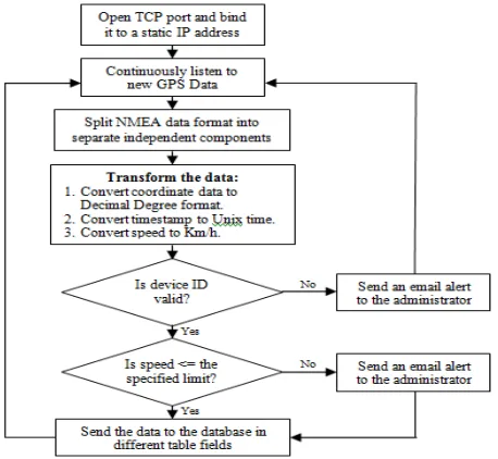
A GPS Data Receiver was developed to receive data that is in $GPRMC sentence format with a MySQL database was used for data storage. Fig. 3 summarizes the functionality of the GPS Data Receiver application that is required to be running all the times.

Fig. 3: The GPS Data Receiver’s functionality

Data interpretation and transformation involves the following:-

1. The data sentence is first split into independent attributes each assigned to a variable based on separators that may include “&” “,” or “#” depending on device manufacturers.

2. Variables holding coordinates data are transformed from Decimal Minute to Decimal Degree format.

3. The two different variables holding date and time data are combined to form a timestamp (dd-mm-yy hh:mm:ss). The timestamp is converted to a Unix time format.

123 Client-Side Applications’ Design

Road Mapping - A Road Mapping table interface was setup to facilitate the mapping of road segments. It functions as per the steps the following two steps:-

1. Determine the length of a road segment to map.

2. Determine the coordinates for a central point for the segment.

3. Update the data in the road map table by filling the road map form. Note that a unique segment name has to be defined for identification of the road segments.

The road map table has the following fields:-

1. Address Code – A unique ID for the road segment.

2. Address – The road mapped segment name.

3. Longitude – The Longitude value for a central point for the road segment.

4. Latitude – The Latitude value for a central point for the road segment.

5. Direction – The direction of movement within the road segment.

6. Length – The length of the road segment.

Algorithm Design

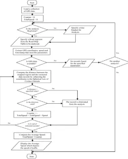
Analyzing data with respect to the road mapped region is key to the determination of the speed of traffic which is a form of data mining targeted at the analysis of status of roads. The flowchart in fig. 4 outlines a speed of traffic analysis algorithm developed in this respect. A road usage pattern analysis algorithm outlined in form of a flowchart in fig. 5 was also developed and implemented for better planning and analysis by the users for instance city planners planning for renovation on a specific road.

Fig. 4: Speed of Traffic analysis algorithm

Fig. 5: Road Usage Pattern algorithm

4. RESULTS

AND

DISCUSSION

GPS Server – Data Format Results

The GPS trackers sends data as one sentence starting with $$ and ending with ##. Sample data sentences received by the GPS Data Receiver are as follows:

$$1000000001???&A9955&B051304.000,A,0116.8618,S, 03645.5808,E,0.00,202.38,280412,,,A*79|0.9|&C0000011 111&D0026:164&E10000000&Y00180000##

124 Table 1: An interpretation of the GPS data sentence

Data Description Parameter

1000000001 Device unique

identifier

Maximum of 15 characters

A9955 Device board ID Manufacturer _specific

051304.000 Time hhmmss.ddd

A Validity of the fix A = Valid

0116.8618 Latitude ddmm.mmmm

S Latitude

hemisphere S = Southern

03645.5808 Longitude dddmm.mmmm

E Longitude

hemisphere E = Eastern

0.00 Speed, knots. s.s

202.38 Course in

degrees h.h

280412 Date ddmmyy

‘$’ ‘,’ ‘?’ ‘&’ and ‘#’

Separator to the various data parameters

The string “A*79|0.9|&C0000011111&D0026:164&E1000 0000&Y00180000” represents proprietary data that the device tracked along the way. This data is usually secreted by the device manufacturers with *79 representing the checksum.

Speed of Traffic Analysis Results

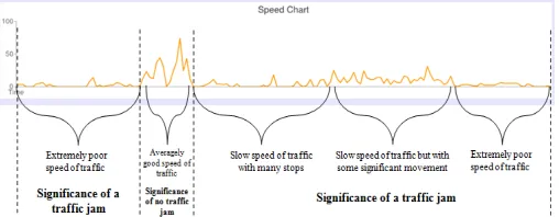
A special algorithm depicted in fig. 4 was developed to determine the speed of traffic whose output is depicted in form of speed charts and a computation of average speed for any given road segment. Fig. 6 shows a sample speed chart.

Fig. 6: Sample speed chart

Using this information from many different vehicles, system users can predict the speed of traffic for any given road segment. Fig. 7 shows a sample traffic speed analysis where vehicle registration numbers Demo and Demo 2 represent the test vehicle with a road mapped segment set to “Langata rd Btw 748 Plaza and Kungu Karumba rd Jct”.

Fig. 7: Output and Speed

The speed charts provided in fig. 6 portray a true picture of an individual vehicle’s movement trend. Based on the detected speed, the Google Chart API incorporated in the application automatically generates a speed chart (a line graph) to summaries the speeding trend. A speed violation email alert is triggered by a higher value speed compared to the set limit. This provides a clear speeding behavior for any given driver hence vital information to the Traffic Police Department and other analysts. Fig. 8 outlines an interpretation and analysis of a sample where two major divisions were detected: traffic jam and no traffic jam. The regions with traffic jam can also be divided based on the wave formed by the chart. This leads to three minor divisions for areas with traffic jam i.e. slow speed of traffic with many stops, slow speed of traffic with some significant movement, and extremely poor speed of traffic.

Fig. 8: An outline of a sample speed chart

The speed data for a group of vehicles subjected to the Speed of Traffic algorithm outlined in fig. 4 leads to the determination of the speed of traffic for any given road mapped segment within a specified time interval. The output of the speed of traffic analysis as illustrated in fig. 7 indicates the following aspects:-

1. The individual vehicle details (the vehicle’s registration number, position coordinates, speed, distance from the mapped region, timestamp for the update, option to view on Google maps).

2. The total number of updates.

3. The total speed.

4. The speed of traffic which is the average speed i.e. the total speed divided by the number of vehicle updates involved.

125

Using the summary of the speed of traffic data, one tell the congestion level by checking on the number of vehicles involved and the speed of traffic by checking on the average speed. The vehicles involved depend on the data points detected within the specified road mapped segment. The distance from the point to the vehicle’s data point is set in the Road Map table depending on the given segment’s distance in Kilometers. This helps to appropriately narrow down on the point of interest. The Spherical Law of Cosines is heavily used in this analysis.

Road Usage Analysis Results

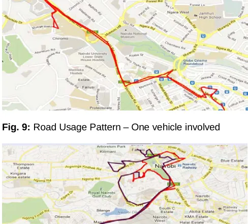
A special algorithm depicted in fig. 5 was developed to determine the road usage pattern which is depicted in form of Google maps for any give point on the map with a specific radius for analysis. Fig. 9 and fig. 10 show sample road usage patterns where the distance from the central point is computed using the Spherical Law of Cosines.

Fig. 9: Road Usage Pattern – One vehicle involved

Fig. 10: Road Usage Pattern – Two vehicles involved

A road usage pattern is generated as waypoints for all vehicles found in a given region determined by a specified centroid point, time interval and radius for analysis. The selected data points are plotted on Google Maps Overlays using polylines. Overlays are objects on the map that are tied to latitude/longitude coordinates, so they move when you drag or zoom the map. Overlays reflect objects that you add to the map to designate points, lines, areas, or collections of objects. The output of the road usage pattern as portrayed in fig. 9 and fig. 10 indicates the waypoint joined by polylines per vehicle. Different colors as depicted in fig. 10 indicate the route used by the different vehicles found within the specified parameters. This is achieved by a random color generator algorithm incorporated in the road usage algorithm. Fig. 9 outlines an analysis done between 2012-6-13 09:50:00 and 2012-6-13 15:00:00. The trace in red outlines two lines that are almost parallel. This is an indicator that the same route was used

from Luthuli Avenue, Nairobi Central Business District to Chiromo Campus and back. Furthermore, fig. 10 depicts a road usage pattern for an analysis involving two vehicles done between 2012-06-20 04:00:00 and 2012-06-22 04:00:00. The trace on the map indicated in red and purple represent two different vehicles that were using the region under analysis within the time interval. Subjecting the analysis to a region with heavy traffic with all vehicles fit with GPS tracking devices would result in as many traces as the vehicles found in that region. This will be a very useful pattern to planners and road users among other analysts. The distance attribute that is required for both the Speed of Traffic and Road Usage analysis is computed using the Spherical Law of Cosines as earlier described. The law uses the specified coordinates and the coordinates in the database to get the distance over a sphere with the Earths radius used. The K-Means algorithm is used in this case where the distance is being subjected to the given centroid. The KNN algorithm is in some way applied in the determination of speed of traffic as follows:-

1. Determine the parameter k = number of nearest neighbors beforehand. In this case, k can range between 0 to n vehicles.

2. Calculate the distance between the query-instance and all the training samples. In this case, we use the Spherical Law of Cosines to calculate the distance.

3. Sort the distances for all the training samples and determine the nearest neighbors based on the K-th minimum distance. In this case, we determine the minimum distance per vehicle based on the data point detected among the k parameter.

4. Since this is supervised learning, we get all the categories of the training data for the sorted value which fall under k.

5. Use the majority of nearest neighbors as the prediction value where in this case we are determining the speed of traffic as our prediction.

The K-Means algorithm is also in some way applied in the determination of road usage patterns in a clustering mode as follows:-

1. Determine the centroid coordinates – We specify the coordinates of our centre of interest for analysis.

2. Determine the distances of each data point to the centroids – We subject the centroid to the Spherical Law of Cosines with respect to all vehicles update data point in question to get the distance between them.

3. Group the data points based on minimum distance – We group the data points based on the radius initially supplied whereby we are only interested in data points less with a distance less than or equal to the radius. At this point, the Google Maps Overlays are then involved for generating the road usage patterns.

Discussion of Results

126

security reasons thus preventing illegal vehicle movement for instance, stolen vehicles or vehicles violating traffic rules.

Algorithms Design and Development

Developing a correct algorithm can be a significant intellectual challenge. Flowcharts which are the most widely used notations for developing algorithms were employed in the development of the two algorithms. This was done independent of the programming language that was used to implement them. Fig. 4 and fig. 5 outlines the two algorithms where the Stepwise Refinement Methodology was used to generate the pseudo-codes for both algorithms. The design of the algorithms considered the preciseness of the algorithms, the algorithms are executable, all possible circumstances are handled and termination of the algorithms. A discussion on the two algorithms is as follows:-

a) The Speed of Traffic Algorithm

The speed of traffic algorithm outlined in fig. 4 works well by utilizing the captured data parameters where it detects the number of vehicles in any given road segment, their direction of movement, the total speed. It then computes the average speed which serves as the speed of traffic. This gives traffic flow information for the road. The algorithm is potential for use if subjected to a set of GPS data containing coordinates, speed, direction and timestamp parameter. In this project, the algorithm was subjected to both historical data and the test data collected after the development of the GPS server.

b) The Road Usage Algorithm

The Road Usage pattern algorithm outlined in fig. 5 works well by utilizing the captured data parameters whereby it detects the vehicles within a given radius and plots the routes the vehicles used in form of polylines. Different colors in each case portray different vehicles. This is termed as a route player that depicts the road usage pattern on Google maps. The algorithm is potential for use if subjected to a set of GPS data containing coordinates and timestamp parameter.

The Model for the System

Fig. 11: The model for the system

The model in fig. 11 has three main sections i.e. the vehicle, the GPS server, and Client-side applications. The GPS server encompasses the GPS Data Receiver and the SQL database while client-side applications encompass the speed of traffic,

road mapping and road usage patterns. The GPS Data Receiver Application was developed to capture the following essential information per vehicle (installed with a GPS tracker) per update which is the source of the data for analysis:-

1. Vehicle registration number

2. Vehicle unique identifier

3. Vehicle current location (GPS coordinates)

4. Vehicle speed received from the tracker’s speed sensors

5. Direction of movement computed as the data streams in

Performance analysis

To rate the performance of the system, predictive and model accuracy tests and analysis were subjected to sample data with conclusions made as follows:

a) Predictive Accuracy

Traffic speed and jams can be termed as dynamic attributes. They can be predictable and also unpredictable based on the situation at hand. A traffic status (speed of traffic) change for a period of 10 minutes can be so magnificent that predicting it may pose a challenge. In Kenya for example, it has been noted that there is a high possibility of heavy traffic jams whenever it rains hence the model may not predict the traffic under such natural circumstances. Peak and off-peak hours can be predicted since this depends on the hour of the day. The system will permit users to analyse and generate reports for traffic flow for instance speeds of traffic.

b) Predictive case for Speed of Traffic

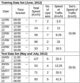
Table 2 and 3 analyses the speed of traffic for the selected road segment (Uhuru Highway between Baricho and Haile Selassie Roundabouts). GPS traffic data gathered in the month of June, 2012 was used as training data sets while May and July, 2012 data sets were used as test data.

Table 2: Uhuru Highway between Baricho and Haile Selassie Roundabouts heading NW

Training Data Set (June, 2012)

Date Time

bracket

Total Speed (Km/h)

No. of Updat

es

Speed of Traffic (Km/h)

Set’s Speed of

Traffic (Km/h)

11/06/12 09:00 –

10:00 36 3 12

7 12/06/12 09:00 –

10:00 61 6 10.17

13/06/12 09:00 –

10:00 15 3 5

22/06/12 13:00 –

14:00 15 18 0.83

Test Data Set (May and July, 2012)

16/05/12 08:00 –

09:00 27 16 6.63

6.51 05/07/12 09:00 –

10:00 27 5 5.4

06/07/12 16:00 –

17:00 72 8 9

12/07/12 14:00 –

127

The analysis from table 2 indicates slow speeds of traffic ranging between 0 and 12 Km/h per given analysis time bracket. The speed of traffic for the test data set resulted to 6.51 Km/h which was very close to 7 Km/h value for the training data set. Under normal circumstances getting into Nairobi town via Uhuru Highway is a common heavy traffic prone area. Traffic speeds ranging between 0 and 12 Km/h can be concluded to be a true picture on the ground for Uhuru Highway between Baricho and Haile Selassie Roundabouts heading NW (i.e. getting into town).

Table 3: Uhuru Highway between Baricho and Haile Selassie Roundabouts heading SE

Training Data Set (June, 2012)

Date Time

bracket

Total Speed (Km/h)

No. of Upd ates

Speed of Traffic (Km/h)

Set’s Speed of

Traffic (Km/h) 12/06/

12

09:00 –

10:00 7 2 3.5

16.66 12/06/

12

17:00 –

18:00 24 2 12

13/06/ 12

18:00 –

19:00 58 7 8.29

21/06/ 12

14:00 –

15:00 66 2 33

23/06/ 12

15:00 –

16:00 53 2 26.5

Test Data Set (May and July, 2012)

16/05/ 12

11:00 –

12:00 127 5 25.4

28.91 30/05/

12

14:00 –

15:00 53 4 13.25

04/07/ 12

09:00 –

10:00 71 2 35.5

06/07/ 12

07:00 –

08:00 83 5 41.5

The analysis from table 3 indicates slightly high speeds of traffic ranging between 12 and 50 Km/h per given analysis time bracket. The speed of traffic for the test data set resulted to 28.91 Km/h which was very close to 16.66 Km/h for the training data set. Under normal circumstances getting out of Nairobi town via Uhuru Highway is a region that experiences fairly good speeds of traffic with minimal stops as compared to the scenario of getting into Nairobi town. Traffic speeds ranging between 12 and 50 Km/h can be concluded to be a true picture on the ground for Uhuru Highway between Baricho and Haile Selassie Roundabouts heading SE (i.e. getting out of town).

Fig. 12: Uhuru Highway between Baricho and Haile Selassie Roundabouts

Fig. 12 depicts a predictive speed of traffic summary for the sample case of Uhuru Highway between Baricho and Haile Selassie Roundabouts. The chart has two main sections i.e. Getting into Town and Getting out of Town with a clear comparison of the training and test data sets used. The data sets used was the similar to the data set used for the analysis in table 2 and 3. It can be evident that getting into town is much slower than getting out of town. A similar convention can be applied to any given road segment with the data gathered by the GPS server developed in this project. It should be noted that the probability of experiencing faster speeds while getting out of town as summarized by chart 1 may not always be true basing on other factors that are unpredictable. Some of these factors may include: accidents, weather conditions, state functions, driver behaviors, state of roads among others.

c) Model Accuracy

The accuracy of the model relies on a number of factors that include: the available GPS signal, the update interval set for the GPS, the time bracket for analysis, the GSM network coverage among others.

5. CONCLUSION

128

of impacts and effectiveness of the measures. For successful implementation of traffic management and control measures, not only should the technical perspectives of the measure be properly considered, but also the integration with existing infrastructure and policies. Based on the test results of the concept, it is recommended that:

1. GPS traffic management are effective, reliable and efficient, with a flexible scale of implementation at relatively small investment, which should be considered as a priority traffic management.

2. Any Nation intending to adopt the model must put in place a policy and/or law prompting all vehicle owners to fit their vehicles with GPS trackers. Furthermore the taxes on importation of the devices should be scraped with prices regulated to help make the devices affordable to the citizens.

3. Some traffic management measures use

sophisticated systems such as safety cameras which cannot be installed all over since they require substantial infrastructure support and fine tuning that is costly to implement. Furthermore, safety cameras can only serve well small parts of a city. GPS systems are less sophisticated to implement hence the better option.

Future research may lie in investigating several enhancements to the current implementation, including automatic traffic prediction with auto alerts to traffic police and drivers detected closer or heading towards congested areas. This prompts for the incorporation of mobile text message alerts as opposed to email alerts. Further research should focus on enhancing the system towards driver behavior analysis and reporting, with specific real-time warnings and advanced mapping, for instance the ability to send a real-time warning alert to the reckless and speeding drivers.

A

Our sincere gratitude goes to Prof. P. W. Wagacha, Mr. J. Ogutu, Mr. D. Orwa and Mr. L. Muchemi for their contribution in critiquing the paper.

R

[1] Auld, J., Williams, C., Mohammadian, A. and Nelson, P. (2008) ‘An automated GPS-based prompted recall survey with learning algorithms’, Journal of Transportation Letters, Chicago.

[2] Biem, A., Bouillet, E., Feng, H., Ranganathan, A., Riabov, A., Verscheure, O. (2010) ‘Real-Time Traffic Information Management using Stream Computing’, IBM TJ Watson Research Center, New York, USA.

[3] Ehmke, J. and Mattfeld, D. (2010) ‘Data allocation and application for time-dependent vehicle routing in city logistics’, European Transport n. 46, pp. 24 – 25, Germany.

[4] Hasan, K., Rahman, M., Haque, A. L., Rahman, M. A., Rahman, T. and Rasheed, M. M. (2009) ‘Cost Effective GPS-GPRS Based Object Tracking System’, Proceedings of the International MultiConference of Engineers and

Computer Scientists 2009, Vol I IMECS 2009, 18 – 20 March, Hong Kong.

[5] Kardashyan, A. (2011) ‘New Concept of the Urban and Inter-Urban Traffic’, Proceedings of the World Congress on Engineering and Computer Science 2011, Vol II, WCECS 2011, 19 – 21 October, San Francisco, USA.

[6] Kochan, B., Bellemans, T., Janssens, D. and Wets, G. (2006) ‘Dynamic activity-travel data collection using a GPS-enabled personal digital assistant’, Proceedings of the ninth International Conference on AATT, pp.319-324.

[7] Marketos, G. (2009) ‘Mobility Data Warehousing and Mining’, 09 Ph D Workshop, 24 August, Lyon, France.

[8] Mukesh, P. and Muruganandham (2010) ‘Real Time Web based Vehicle Tracking using GPS’, World Academy of Science, Engineering and Technology 61.

[9] Owusu, J., Afukaar, F. and Prah, B. E. K. (2006) ‘Urban Traffic Speed Management: The Use of GPS/GIS’, Shaping the Change, XXII FIG Congress, Munich, Germany 8-13.

[10] Thianniwet, T., Phosaard, S., member, IAENG, and Pattara-Atikom, W. (2009) ‘Classification of Road Traffic Congestion Levels from GPS Data using a Decision Tree Algorithm and Sliding Windows’, Proceedings of the World Congress on Engineering 2009, Vol I, WCE 2009, 1 – 3 July, London, U.K.

[11] Tripathi, J. (2010) Algorithm for Detection of Hot Spots of Traffic through Analysis of GPS Data. Thesis submitted in partial fulfillment of the requirement for the award of degree of Master in Engineering in Computer Science and Engineering. Thapar University, Patiala.

[12] Ye, Q., Chen, L. and Chen, G. (2009) ‘Personal Continuous Route Pattern Mining’, Journal of Zhejiang University Science A, 2009 10(2): pp. 221 – 231, Hangzhou 310027, China.