Optimization of Material Removal Rate and Surface Roughness using Grey Analysis

e-ISSN: 2278-067X, p-ISSN: 2278-800X, www.ijerd.com

Volume 12, Issue 3 (March 2016), PP.49-58

Optimization of Material Removal Rate and Surface Roughness

using Grey Analysis

Ch.Maheswara Rao

, K.Jagadeeswara Rao

, K.Suresh babu

1

Department of Mechanical Engineering, Raghu Institute of Technology, Dakamarri, Visakhapatnam, INDIA

2

Department of Mechanical Engineering, Aditya Institute of Technology and Management, Tekkali, INDIA

3

Department of Mechanical Engineering, Raghu Institute of Technology, Dakamarri, Visakhapatnam, INDIA

Abstract:- Medium carbon steel EN19 has wide range of applications in the manufacturing industries. It is used for preparing studs, high tensile bolts, riffle barrels and propeller shafts etc. The present work is to investigate the influence of machining parameters on Material Removal Rate and Surface Roughness characteristics Ra and

Rz. The experiments were conducted as per standard Taguchi‟s L9 orthogonal array. For multi objective

optimization of the responses, Taguchi based grey relational grade method was adopted. From multi objective grey analysis, the optimal combination of process parameters was found at speed: 225 m/min, feed: 0.05 mm/rev, and depth of cut: 0.6 mm.The assumptions of ANOVA like Normal distribution, constant variance and independence of residuals are verified with the residual plots drawn for the responses using MINITAB-16 software. From ANOVA results, it is clear that speed has more significance in affecting the multi responses and followed by depth of cut and feed. The mathematical models were prepared for the individual responses by using regression analysis and a close relation between the predicted values from models and experimental values was observed.

Keywords:- EN19 steel, Taguchi, Regression Analysis, Grey Analysis, Material removal rate, Surface roughness, ANOVA.

I.

INTRODUCTION

The challenge of modern machining industries is mainly focussed on achieving high quality, in terms of high production rate, surface finish and dimensional accuracy. Highproduction rate can be achieved through conventional machining methods but high production with better surface finish can be achieved through non conventional machining only. So, the use of non conventional methods has been increased in present manufacturing industries.Surface roughness most commonly refers to the variations in the height of the surface relative to a reference plane. It is usually characterised by one of the two statistical height descriptors advocated by the American National Standards Institute (ANSI) and the International Standardisation Organisation (ISO). They are one is Ra, CLA (Centre Line Average) or Arithmetic average and two is standard deviation (Rq) or

Root Mean Square (RMS). Two other statistical height descriptors are Skewness (SK) and Kurtosis (K). Other

measures of surface roughness height descriptors are, Rt-Extreme value height descriptor (Ry, Rmax, or maximum

peak to valley height), Rp -Maximum peak height or maximum peak to mean height, Rv- maximum valley depth

or mean to lowest valley height, Rz- average peak-to-valley height, and Rpm- Average peak to mean height etc.

Among all Ra, Rq and Rz are surface topology parameters which are very significant from contact stiffness,

fatigue strength and surface wear point of view. Surface roughness of the product has a significant effect on functional attributes of parts, like surface friction while contact, wearing, light reflection, ability of distributing and holding a lubricant and resistant fatigue etc. There are many factors which affect the Surface Roughness and Material Removal Rate such as cutting conditions, tool variables and work piece variables. Cutting conditions include speed, feed and depth of cut. Tool variables include tool material, nose radius, rake angle, cutting edge geometry, tool vibrations, tool overhang, tool point angle etc and work piece variable include hardness, mechanical and physical properties of material.[1-5] For improving the surface quality of parts now a day‟s Tungsten carbide tools are using because of their advantages like high speed, high surface finish, high hardness, low friction coefficient, low thermal conductivity and low thermal expansion, reduction in tool wear, reduction in built up edge formation etc.[6]

Analysis of variance was used to find the significance of the process parameters on the responses. [9-10] Regression models for the responses were prepared by using MINITAB-16 software. The models were checked for their accuracy and adequacy using normal probability, versus fits and versus order plots. Finally, predicted values calculated from the models were compared with experimental values and the Comparison graphs for the responses were drawn by using EXCEL. [11-12]

II. EXPERIMENTAL SETUP

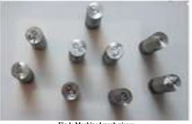
For experiment, the work piece of EN19 each of 25 mm diameter and 75 mm length has been taken. The experiment has been performed on CNC lathe (Jobber XL, 7.5Kw, 50-4000 rpm) under dry conditions using Tungsten carbide tool. The chemical composition, physical and mechanical properties of EN19 steel were given in the tables 1 and 2. Material removal rate is calculated by multiplying cutting parameters speed, feed and depth of cut is measured in cm3/min. For the finished products surface roughness values were measured by using SJ-301 (Mututoyo) gauge at three different places and the average was taken as Roughness value. The machined work pieces were shown in the Fig. 1.

Table 1:Chemical composition of EN19 material

Element C Si Mn Cr Mo S P

% Weight 0.36-0.44 0.1-0.35 0.7-1 0.9-1.2 0.25-0.35 0.035 0.040

Table 2: Mechanical properties of EN19 material Density

(g/cm3)

Tensile strength (N/mm2)

Yield strength (N/mm2)

Elongation (%)

Izod (J)

Hardness (BHN)

7.7 850-1000 680 13 50 248-302

Experimental conditions:

Material : Medium carbon steel EN19

Machine : CNC lathe (Jobber XL, 7.5Kw, 50-4000 rpm) Cutting tool : Tungsten carbide

Insert : DNMG 160404 Tool holder: PDJNL2525M16

Surface Roughness guage : SJ-301 (Mututoyo) Environment : Dry

Fig.1: Machined work pieces

III.

METHODOLOGY

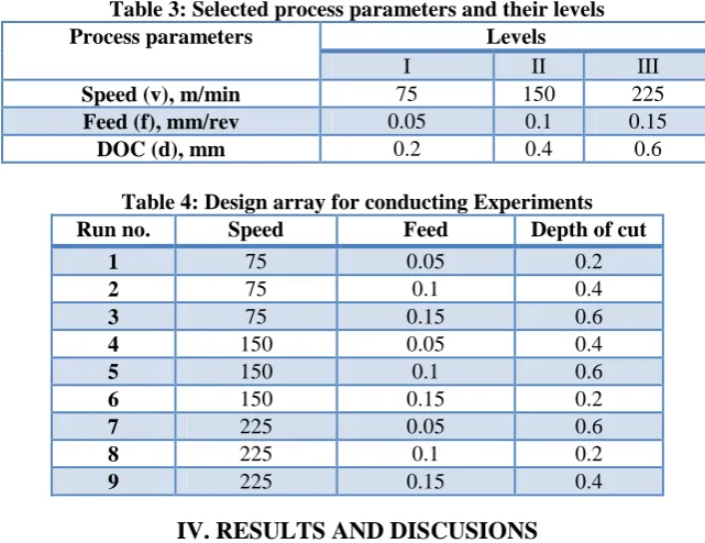
invented. Grey method deals with the systems in which part of information is known and part of information is unknown. This method converts the multi-objective problem into a single objective problem in terms of Grey relational grade. [13-16] The selected process parameters with their levels and Orthogonal Array with actual experimental values were given in the tables 3 and 4. The steps involved in Grey analysis are

1. Identification of responses (MRR, Ra and Rz) and input parameters (Speed, feed and depth of cut).

2. Determine the different levels (3) for the input parameters.

3. Selection of appropriate Orthogonal Array (L9) and assign the process parameters.

4. Carry out the experiment as per L9 Orthogonal Array.

5. Normalization of responses.

6. Finding out the grey relational generation and grey relational coefficient (GRC).

7. Calculation of Grey relational grade (GRG).

8. Analyze the grey relational grade.

9. Selection of optimal combination of process parameters.

Table 3: Selected process parameters and their levels

Process parameters Levels

I II III

Speed (v), m/min 75 150 225

Feed (f), mm/rev 0.05 0.1 0.15

DOC (d), mm 0.2 0.4 0.6

Table 4: Design array for conducting Experiments

Run no. Speed Feed Depth of cut

1 75 0.05 0.2

2 75 0.1 0.4

3 75 0.15 0.6

4 150 0.05 0.4

5 150 0.1 0.6

6 150 0.15 0.2

7 225 0.05 0.6

8 225 0.1 0.2

9 225 0.15 0.4

IV. RESULTS AND DISCUSIONS

The objective of the present work is to find the optimum combination of process parameters for which both MRR and Surface roughness characteristic values are to be optimized. The experimental results of Material Removal rate and Surface roughness parameters Ra and Rz values were calculated and given in the table 5.

Table 5: Experimental results of responses

S.No. Experimental results

MRR Ra Rz

1 0.75 2.6 12.6

2 3 3.1 14.2

3 6.75 3.7 15.3

4 3 1.8 6.4

5 9 2.3 9.8

6 4.5 2.8 12.8

7 6.75 0.9 4.1

8 4.5 1.6 7.6

9 13.5 2.1 9.7

Grey relational generation

Grey relational generation includes, normalizing the experimental values yij as Zij (0≤Zij≤1) by following

formulae to reduce variability. Grey relational generation values of responses were given in the table 6.

Zij =

Yij−min Yij,i=1,2,….,n

max Y_ij,i=1,2,….,n −min Y_ij,i=1,2,…..,n ; Used for Material Removal Rate.

Zij =

max Y_ij,i=1,2,….,n −Y_ij

max Y_ij,i=1,2,……,n −min Y_ij,i=1,2,…..,n ; Used for Surface Roughness parameters (Ra and Rz).

Table 6: Grey relation generation

S. No. Grey relational generation

MRR Ra Rz

1 0.000 0.393 0.241

2 0.176 0.214 0.098

3 0.471 0.000 0.000

4 0.176 0.679 0.795

5 0.647 0.500 0.491

6 0.294 0.321 0.223

7 0.471 1.000 1.000

8 0.294 0.750 0.688

9 1.000 0.571 0.500

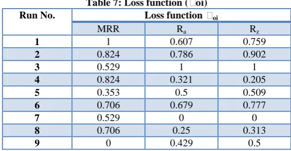
Loss function

Loss function can be calculated by using, Delta (∆) = (Quality loss) = 𝑦𝑜− 𝑦𝑖𝑗 ; the values were given in the

table 7.

Table 7: Loss function (∆oi)

Run No. Loss function ∆oi

MRR Ra Rz

1 1 0.607 0.759

2 0.824 0.786 0.902

3 0.529 1 1

4 0.824 0.321 0.205

5 0.353 0.5 0.509

6 0.706 0.679 0.777

7 0.529 0 0

8 0.706 0.25 0.313

9 0 0.429 0.5

Grey relational coefficient

GRC can be calculated using below formulae and the values were given in the table 8.

GCij=

∆min +δ∆max

∆ij+δ∆max

i = 12, … . n j = 1,2, … k

Where, GCij= grey relational coefficient for the ith replicate of jth response.

∆= quality loss │Y0-Yij│

∆min= minimum value of ∆

∆max= maximum value of ∆

δ = distinguishing coefficient which is in range of 0≤δ≤1 (normally δ=0.5)

Grey relational grade

`GRG can be calculated by using below formulae and the values were given in the table 8.

Gi=

1

m GCij; Where GC is Grey relational coefficient of responses and m is total number of responses.

Table 8:Grey relational coefficient and grade

Run No. Grey relational coefficient Grey

relational grade

S/N ratios of GRG

Rank

MRR Ra Rz

1 0.333 0.452 0.397 0.394 -8.0900 7

2 0.378 0.389 0.357 0.374 -8.5425 9

3 0.486 0.333 0.333 0.384 -8.3133 8

4 0.378 0.609 0.709 0.565 -4.9590 4

5 0.586 0.500 0.496 0.527 -5.5637 5

6 0.415 0.424 0.392 0.410 -7.7443 6

7 0.486 1 1 0.829 -1.6289 1

8 0.415 0.667 0.615 0.566 -4.9436 3

9 1.000 0.538 0.5 0.679 -3.3626 2

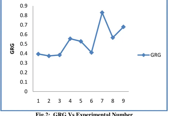
Graph is plotted by taking Experimental number on X-axis and Grey relational grade on Y-axis and shown in the Fig. 2. From the figure, it is observed that seventh experiment gives the best multi performance characteristics among the nine experiments.

Fig.2: GRG Vs Experimental Number

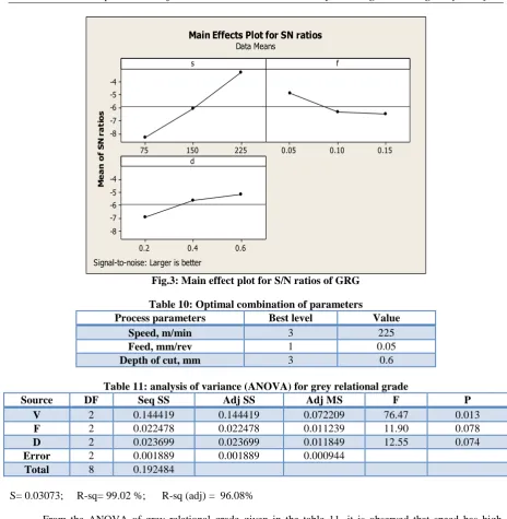
The mean S/N ratio values were calculated for Grey relational grade and given in the table 9. From, mean S/N ratio values and main effect plot for the grey relational grade was drawn and shown in the Fig. 3. From the figure a significant change in value of GRG can be observed with the change in levels of speed. Similarly, this change is less with the change in levels of feed and depth of cut. From mean S/N ratio table, it is clear that Speed is the most significant factor affecting the multiple performance characteristics followed by depth of cut and feed. The optimal combination of process parameters with their levels and values were given in the table 10.

Table 9: Response for mean grey relational grade

Factors Mean relational grade Max-min Rank

Level-1 Level-2 Level-3

v -8.315 -6.089 -3.312 5.004 1

f -4.893 -6.350 -6.473 1.581 3

d -6.926 -5.621 -5.169 1.757 2

0 0.1 0.2 0.3 0.4 0.5 0.6 0.7 0.8 0.9

1 2 3 4 5 6 7 8 9

GR

G

225 150

75 -4 -5 -6 -7 -8

0.15 0.10

0.05

0.6 0.4

0.2 -4 -5 -6 -7 -8

s

M

e

a

n

o

f

S

N

r

a

ti

o

s

f

d

Main Effects Plot for SN ratios

Data Means

Signal-to-noise: Larger is better

Fig.3: Main effect plot for S/N ratios of GRG

Table 10: Optimal combination of parameters

Process parameters Best level Value

Speed, m/min 3 225

Feed, mm/rev 1 0.05

Depth of cut, mm 3 0.6

Table 11: analysis of variance (ANOVA) for grey relational grade

Source DF Seq SS Adj SS Adj MS F P

V 2 0.144419 0.144419 0.072209 76.47 0.013

F 2 0.022478 0.022478 0.011239 11.90 0.078

D 2 0.023699 0.023699 0.011849 12.55 0.074

Error 2 0.001889 0.001889 0.000944

Total 8 0.192484

S= 0.03073; R-sq= 99.02 %; R-sq (adj) = 96.08%

From the ANOVA of grey relational grade given in the table 11, it is observed that speed has high significance (F = 76.47) for achieving the high material removal rate and low surface Equality characteristics taken together followed by depth of cut and feed.

4.1 Regression Analysis

The relation between the output and input parameters can be found by using regression analysis. The Mathematical models for the responses were prepare by using MINITAB-16 software and given below

MRR = - 8.00 + 0.0317 s + 47.5 f + 10.6 d Ra = 2.86 - 0.0107 s + 11.0 f - 0.083 d Rz = 13.5 - 0.0460 s + 49.0 f - 3.17 d

4 3 2 1 0 -1 -2 -3 -4 99 95 90 80 70 60 50 40 30 20 10 5 1 Residual P e rc e n t

Normal Probability Plot (response is MRR)

12 10 8 6 4 2 0 3 2 1 0 -1 -2 Fitted Value R e si d u a l Versus Fits (response is MRR)

Fig.4: Normal probability plot for MRR Fig.5: Versus fits plot for MRR

9 8 7 6 5 4 3 2 1 3 2 1 0 -1 -2 Observation Order Re si du al Versus Order (response is MRR)

Fig.6: Versus order plot for MRR

0.10 0.05 0.00 -0.05 -0.10 99 95 90 80 70 60 50 40 30 20 10 5 1 Residual P e rc e n t

Normal Probability Plot (response is Ra)

4.0 3.5 3.0 2.5 2.0 1.5 1.0 0.050 0.025 0.000 -0.025 -0.050 -0.075 -0.100 Fitted Value R e s id u a l Versus Fits (response is Ra)

Fig.7: Normal probability plot for Ra Fig.8: Versus fits plot for Ra

9 8 7 6 5 4 3 2 1 0.050 0.025 0.000 -0.025 -0.050 -0.075 -0.100 Observation Order Re sid ua l Versus Order (response is Ra)

1.5 1.0 0.5 0.0 -0.5 -1.0 -1.5 99

95 90 80 70 60 50 40 30 20 10 5

1

Residual

P

e

rc

e

n

t

Normal Probability Plot (response is Rz)

15.0 12.5 10.0 7.5

5.0 1.0

0.5

0.0

-0.5

-1.0

-1.5

Fitted Value

R

e

si

d

u

a

l

Versus Fits (response is Rz)

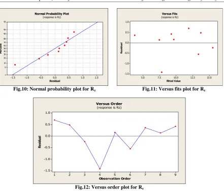
Fig.10: Normal probability plot for Rz Fig.11: Versus fits plot for Rz

9 8 7 6 5 4 3 2 1 1.0

0.5

0.0

-0.5

-1.0

-1.5

Observation Order

Re

si

du

al

Versus Order (response is Rz)

Fig.12: Versus order plot for Rz

From the Regression models, predicted values for MRR, Ra and Rz were calculated and given in the

table 12. The predicted values were compared with the experimental values and comparison graphs were drawn by taking experiment number on X- axis and response on Y-axis and shown in figures 13 to 15. From the results, it is found that both experimental and regression values are close to each other hence, regression models prepared are more accurate and adequate.

Table 12: Comparison of experimental and predicted values of responses

S.No MRR Ra Rz

Experimental predicted Experimental predicted Experimental predicted

1 0.75 -1.13 2.6 2.59 12.6 11.87

2 3 3.37 3.1 3.12 14.2 13.68

3 6.75 7.86 3.7 3.66 15.3 15.5

4 3 3.37 1.8 1.77 6.4 7.78

5 9 7.87 2.3 2.31 9.8 9.6

6 4.5 6 2.8 2.89 12.8 13.32

7 6.75 7.87 0.9 0.95 4.1 3.7

8 4.5 6 1.6 1.54 7.6 7.42

Fig.13: Comparison plot for MRR

Fig.14: Comparison plot for Ra

Fig.15: Comparison plot for Rz

-2 0 2 4 6 8 10 12 14 16

1 2 3 4 5 6 7 8 9

M

R

R Experimental

Predicted

0 0.5 1 1.5 2 2.5 3 3.5 4

1 2 3 4 5 6 7 8 9

Ra Experimental

Predicted

0 2 4 6 8 10 12 14 16 18

1 2 3 4 5 6 7 8 9

Rz Experimental

V. CONCLUSIONS

From the experimental and regression results the following conclusions can be drawn.

 From multi objective grey analysis, the optimal combination of process parameters was found at speed: 225 m/min, feed: 0.05 mm/rev, and depth of cut: 0.6 mm.

 From ANOVA results, it is clear that speed has more significance in affecting the responses and followed by depth of cut and feed.

 Mathematical models developed for the responses were more accurate and adequate and they can be used for the prediction of responses.

REFERENCES

[1]. Upinder Kumar Yadav., Deepak Narang., Pankaj Sharma Attri., “Experimental Investigation and optimization of machining parameters for surface roughness in CNC turning by Taguchi method”; IJERA; ISSN:2248-9622; Vol.2, Issue4, pp.2060-2065, 2012.

[2]. H.K.Dave et.al. “Effect of machining conditions on MRR and Surface Roughness during CNC Turning

of different materials using TiN Coated Cutting Tools by Taguchi method”, International Journal of IndustrialEngineeringComputations3,pp.925-930,2012.

[3]. Harish Kumar., mohd. Abbas., Dr. AasMohammad, Hasan Zakir Jafri.,“optimization of cutting parameters in CNC turning”; IJERA; ISSN:2248-9622; Vol.3, Issue3, pp.331-334, 2013.

[4]. M.Kaladhar et.al. “Determination of Optimal Process parameters during turning of AISI304 Austenitic Stainless Steel using Taguchi method and ANOVA”, International Journal of Lean Thinking, Volume 3, Issue 1, 2012.

[5]. Harish singh & Pradeep kumar, “optimizing feed force for turned parts through the Taguchi technique”, Sadana vol.31, part 6, pp. 671-681, 2006.

[6]. N.E. Edwin Paul, P. Marimuthu, R.Venkatesh Babu; “Machining parameter setting for facing EN 8 steel with TNMG Insert”; American International Journal of Research in Science and Technology, Engineering & Mathematics, 3(1),pp.87-92, 2013.

[7]. Bhaskar reddy. C, Divakar reddy.V, Eswar reddy.C, “Experimental Investigations on MRR and Surface roughness of EN19 & SS420 steels in wire EDM using Taguchi method”, International Journal of Engineering Science and Technology, 4(11), pp. 4603-14, 2012.

[8]. M.Kaladhar, K. Venkata Subbaiah, Ch.Srinivasa Rao and K.Narayana Rao, “Application of Taguchi Approach and utility concept in solving the Multi-objective problem when turning AISI 202 Austenitic Stainless Steel”, Journal of Engineering and technology Review (4), pp.55-61, 2011.

[9]. Huang J.T. and Lin J.L., “Optimization of Machining parameters setting of EDM process based on Grey relational analysis with L18 Orthogonal Array”, Journal of Technology, 17:pp.659-664, 2002.

[10]. Kamal Jangra, Sandeep Grover and Aman Aggarwal, “Simultaneous optimization of material removal

rate and surface roughness for WEDM of WCCo composite using grey relational analysis along with Taguchi method”, International journal of industrial engineering computations 2, pp. 479-490, 2011. [11]. Kanlayasiri , K. , Boonmung , S., „„Effects of wire- EDM machining variables on surface roughness of

newly developed DC 53 die steel: Design of experiments and re- gression model‟‟, Journal of materials Processing Technology, vol. 192–193, pp. 459–464, 2007.

[12]. Dipti Kanta Das, Ashok Kumar Sahoo, Ratnakar Das, B.C.Routara “Investigations on hard turning using coated carbide insert: Grey based Taguchi and regression methodology” Elsvier journal, procedia material science 6, pp. 1351-1358, 2014.

[13]. Mohit Tiwari, Kumar Mausam, Kamal Sharma and Ravindra Pratap Singh “Investigate the Optimal combination of process parameters for EDM by using a Grey Relational Analysis”, Elsvier journal, procedia material science5, pp. 1736-1744, 2014.

[14]. Huang J.T. and Lin J.L., “Optimization of Machining parameters setting of EDM process based on Grey relational analysis with L18 Orthogonal Array”, Journal of Technology, 17, pp. 659-664, 2002.

[15]. Vikas, Apurba Kumar Roy, Kaushik Kumar “Effect and Optimization of Machine Process Parameters

on Material Removal Rate in EDM for EN41 Material Using Taguchi”, International Journal of Mechanical Engineering and Computer Applications, vol. 1, Issue 5, pp. 35-39, 2013.