Mining Frequent Itemsets Based On CBSW Method

e-ISSN : 2278-067X, p-ISSN : 2278-800X, www.ijerd.com

Volume 2, Issue 7 (August 2012), PP. 80-84

Mining Frequent Itemsets Based On CBSW Method

K Jothimani

, Dr Antony SelvadossThanmani

PhD Research Scholar, NGM College,Pollachi, Tamilnadu,India 2

Associate Professor and Head, NGM College,Pollachi, Tamilnadu,India

Abstract—Mining data streams poses many newchallenges amongst which are the one-scan nature, the

unboundedmemory requirement and the high arrival rate of data streams.In this paper we propose a Chernoff Bound based Sliding-window approach called CBSW which is capable of mining frequent itemsets over high speed data streams.In the proposed method we design a synopsis data structure to keeptrack of the boundary between maximum and minimum window size prediction for itemsets. Conceptual drifts in a data streamare reflected by boundary movements in the data structure. The decoupling approach of simplified Chernoff bound defines the boundary limit for each transaction. Our experimental results demonstrate the efficacy of the proposed approach.

Keywords—Chernoff Bound, Data Streams, Decoupling, Mining Frequent Itemsets

I.

INTRODUCTION

Frequent itemset mining is a traditional and importantproblem in data mining. An itemset is its support is not less than a threshold specified byusers. Traditional frequent itemset mining approacheshave mainly considered the problem of mining statictransaction databases [1].Many applications generate largeamount of data streams in real time, such as sensor datagenerated from sensor networks, online transaction flowsin retail chains, Web record and click-streams in Webapplications, call records in telecommunications, and performancemeasurement in network monitoring and trafficmanagement. Data streams are continuous, unbounded, usually come with high speed and have a data distributionthat often changes with time. Hence, it is also calledstreaming data [5].

Nowadays, data streams are gaining more attention as they are one of themost used ways of managing data such as sensor data that cannot be fullysystemsupervision (e.g. web logs), require novel approaches for analysis. Somemethods have been defined to analyse this data, mainly based on sampling,for extracting relevant patterns [5, 10]. They have to tackle the problem ofhandling the high data rate, and the fact that data cannot be stored andhas thus to be treated in a one pass manner [1].

With the rapid emergence of these new application domains, it has become increasingly difficult to conduct advanced analysis and data mining over fast-arriving and large data streams in order to capture interesting trends, patterns and exceptions.From the last decade, data mining, meaning extracting useful information or knowledge from largeamounts of data, has become the key technique to analyse and understand data. Typical data miningtasks include association mining, classification, and clustering. These techniques help find interestingpatterns, regularities, and anomalies in the data. However, traditional data mining techniques cannot directly apply to data streams. This is because mining algorithms developed in the past target disk residentor in-core datasets, and usually make several passes of the data.

Unlike mining static databases, mining data streams poses many new challenges. First, itis unrealistic to keep the entire stream in the main memory or even in a secondary storagearea, since a data stream comes continuously and the amount of data is unbounded. Second, traditional methods of mining on stored datasets by multiple scans are infeasible, since thestreaming data is passed only once. Third, mining streams requires fast, real-time processingin order to keep up with the high data arrival rate and mining results are expected to be availablewithin short response times. In addition, the combinatorial explosion1 of itemsets exacerbatesmining frequent itemsets over streams in terms of both memory consumption and processingefficiency. Due to these constraints, research studies have been conducted on approximatingmining results, along with some reasonable guarantees on the quality of the approximation[6].

For the window-based approach, we regenerate frequent itemsets from the entire windowwhenever a new transaction comes into or an old transactionleaves the window and also store every itemset, frequent or not, in a traditionaldata structure such as the prefix tree, and update itssupport whenever a new transaction comes into or anold transaction leaves the window.[20]In fact, as long asthe window size is reasonable, and the conceptual drifts inthe stream is not too dramatic, most itemsets do not changetheir status (from frequent to non-frequent or from non-frequentto frequent) often. Thus, instead of regeneratingall frequent itemsets every time from the entire window, weshall adopt an incremental

approach.

II.

RELATED

WORK

In a sliding window model, knowledge discovery isperformed over a fixed number of recently generated dataelements which is the target of data mining. Two types ofsliding widow, i.e., transaction-sensitive sliding windowand time-sensitive sliding window, are used in mining datastreams. The basic processing unit of window sliding oftransaction-sensitive sliding window is an expired transactionwhile the basic unit of window sliding of time-oftransaction-sensitivesliding window is a time unit, such as a minute or 1 h.The sliding windowcan be very powerful and helpful when expressing some complicated mining tasks with a combination of simple queries[17].

For instance, the itemsets with a large frequency change can be expressed bycomparing the current windows or the last window with the entire time span. For example, the itemsetshave frequencies higher than 0.01 in the current window but are lower than 0.001 for the entire timespan. However, to apply this type of mining, mining process needs different mining algorithms fordifferent constraints and combinations.[15,18] The flexibility and power of sliding window model can makethe mining process and mining algorithms complicated and complex. To tackle this problem, wepropose to use system supports to ease the mining process, and we are focusing on query languages,system frameworks, and query optimizations for frequent itemset mining on data streams.

Continuous sliding-window queries over data streams havebeen introduced to limit the focus of a continuous query toa specific part of the incoming streamtransactions. The window-of-interest in the sliding-window querymodel includes the most-recent input transactions. In a slidingwindowquery over n input streams, S1 to Sn, a windowof size wiis defined over the input stream Si. The slidingwindowwican be defined over any ordered attribute in the stream tuple.As the window slides, the query answer is updatedto reflect both the new transactions entering the sliding-windowand the old transactions expiring from the sliding-window. Transactionsenter and expire from the sliding-window in a First-In-First-Expire (FIFE) fashion.

III.

CHERNOFFBOUND

BASED

SLIDING

WINDOW(CBSW)

ALGORITHM

In this section we present our CBSW algorithm. CBSW uses the simplified Chernoff bound concepts to calculate the appropriate window size for mining frequent itemsets. It then uses the comparison of the two window sub-range observations and itemset counts when a transition occurs within the window and then adjusts the window size appropriately.

A. Window Initialization using Binomial Sampling

CBSW is able to adapt its window size to cope with a more efficient transition detection mechanism. It viewed as an independent Bernoulli trial (i.e., a sample draw for tag i) with success probability pi,t using Equation (1) [16]. This implies

that the number of successful observations of items i in the window Wi with epochs (i.e., Wi= (t – wi, t)) is a random variable with a binomial distribution B(wi, pi,t). In the general case, assume that item i is seen only in subset of all epochs in the

window Wi. Assuming that, the item probabilities within an approximately sized window calculated using Chernoff, are relatively homogeneous, taking their average will give a valid estimate of the actual probability of tag i during window Wi

[16].

The derived binomial sampling model is then used to set the window size to ensure that there are enough epochs in the window Wi such that tag i is read if it does exist in the reader’s range. Setting the number of epochs within the smoothing

window according to Equation (3) ensures that tag i is observed within the window Wi with probability >1 – δ [16]

Wi ≥ [ ( 1/ pi avg

) ln (1/ δ)]………..(1)

B. Window Size Adjustment

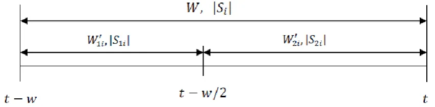
In order to balance between guaranteeing completeness and capturing tag dynamics the CBSW algorithm uses simple rules, together with statistical analysis of the underlying data stream, to adaptively adjust the cleaning window size. Assume Wi = (t - wi, t) is tag i current window, and let W1i′ = (t - wi, t - wi/2) denote the first half of window Wi and W2i′ = (t - wi/2, t) denote the second half of the window Wi. Let |S1i| and|S2i| denote the binomial sample size during W1i′ and W2i′respectively. Note that the mid value in inclusive on both range as shown in Figure 1.

Figure 1.Illustration of the transaction itemsets in the smoothing window.

The window size is increased if the computed window size using Equation (1) is greaterthan the current window size and the expected number of observation samples(|Si|>wipiavg)is less than the actual number of observed samples. Low expected observation samples indicates that the probability of detection ispi

avg

low, in this case we need to grow the window size to give more opportunity for the poor performing tag to be detected. Otherwise, if the expected observation sample is equal or greater than the actual sample size it means that, thepi

avg

bound method. Initially all new transactions are stored into windows and whenever high speed data stream arrives the window size will be automatically regenerated.

The CBSW Algorithm

Input: T = set of all observed transaction IDs δ = required data streams

Output: t = set of all present frequent itemset IDs Initialise:∀𝑖 ∈ 𝑇, 𝑤𝑖← 1

while(getNextTransaction) do for(i in T)

processWindow(Wi) →,pi,t’s, piavg ,|Si|

if(itemExist(|Si|)

outputi end if

wi* ← requiredWindowSize(piavg,δ) if(itemexists^ |S2i| = 0)

wi←max (min{wi/2,wi *

} , 3)

else if (detectTransaction(|Si|,wi,piavg)) wi← max{(wi- 2),3}

else if (wi* >wi^ |Si|<wipiavg)

wi←min{(wi+ 2),wi *

} end if

end for end while

Also we observed the variation within the windowcould also be caused by missing itemsets and it is not necessarily happened only due to transition. Hence, to reduce thenumber of false positive due to transition and the number of false negative readings, which will befurther introduced in case of wrong transition detection, the window size is reduced additively byreducing the window size.Setting the minimum window size can be balanced between maintaining thesmoothing effect of the algorithm and reducing the false positive errors. Similar to FIDS, CBSWalso slides its window per single transaction and produces output readings corresponding to themidpoint of the window after the entire window has been read.

IV.

EXPERIMENTAL

RESULTS

In this section we present our experimental evaluation of the proposed CBSW algorithm.The data sets for our experiments were generated by a synthetic data generator that simulates theoperation of mining frequent itemset readers under a wide variety of conditions using MATLAB. The generator iscomposed of two components. The first component simulates the movement of transactions and the second component simulates itemset detection.

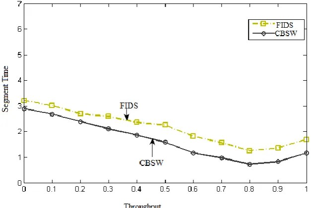
First, we compare the performance effectiveness between the CBSW algorithm and FIDSusing the generated synthetic data sets.As shown in this figure 1, the proposed algorithm has the better runtime for different minimumsupport values. As the minimum support threshold decreases, the performance gap of ouralgorithm with respect to the other methods increases. The reason is, for lower minimum supportthresholds, the number of frequent itemsets is increased.

Fig. 2 Example of an image with acceptable resolution

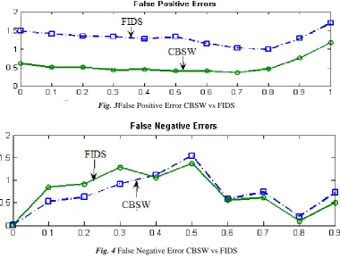
Figure 2shows the result of transaction itemsets for different window sizes. Figure 3, 4 shows their positive and negative error contributions.

Fig. 3False Positive Error CBSW vs FIDS

Fig. 4 False Negative Error CBSW vs FIDS

V.

CONCLUSIONS

REFERENCES

[1]. C.Raissi, P. Poncelet, Teisseire, “Towards a new approach for miningfrequent itemsets on data stream”, J IntellInfSyst , 2007, vol. 28, pp.23–36, 2007.

[2]. J,.Xu Yu , Z.Chong , H. Lu, Z. Zhang , A. Zhou b,” A false negativeapproach to mining frequent itemsets from high speed transactional datastreams”, Information Sciences 176, 1986–2015,2006.

[3]. G. Giannella, J. Han, J. Pei, X. Yan, P.Yu,” Mining frequent patterns indata streams at multiple time granularities”, In Next generation datamining. New York: MIT, 2003.

[4]. H. Li, F. Lee, S.Y., M. Shan,” An efficient algorithm for mining frequentitemsets over the entire history of data streams”.,In Proceedings of the1st InternationalWorkshop on Knowledge Discovery in Datastreams,2004.

[5]. R. Jin, G. Agrawal,” An Algorithm for In-Core Frequent Itemset Miningon Streaming Data”

[6]. P. Domingos , G. Hulten,” Mining high-speed data streams”,InProceedings of the ACM Conference on Knowledge and DataDiscovery (SIGKDD), 2000.

[7]. A. Cheng, Y. Ke,W. Ng, “A survey on algorithms for mining frequentitemsets over data streams”, KnowlInfSyst, 2007. [8]. M. Charikar, K. Chen, M. Farach,” Finding frequent items in datastreams”. Theory ComputSci, vol. 312, pp.3–15, 2004. [9]. R.Agrawal,T. Imielinski,A. Swami , “Mining association rules betweensets of items in large databases”, In Proceedings of the

ACM SIGMODinternational conference on management of data, Washington DC, pp207–216,1993.

[10]. H. Chernoff, A measure of asymptotic efficiency for tests of ahypothesis based on the sum of observations, The Annals ofMathematical Statistics 23 (4) 493–507, 1953.

[11]. M. Charikar, K. Chen, M. Farach,” Finding frequent items in datastreams”, in Proceedings of the International Colloquium on Automata,Languages and Programming (ICALP), pp. 693–703,2002.

[12]. T. Calders , N. Dexters , B. Goethals ,“Mining Frequent Items in aStream Using Flexible Windows” [13]. X. Sun Maria, E. Orlowska , X. Li, “Finding Frequent Itemsets in High-Speed Data Streams”.

[14]. X. Han Dong, W. Ng, K. Wong,V. Lee, “Discovering Frequent Setsfrom Data Streams with CPU Constraint”, This paper appeared at theAusDM 2007, Gold Coast, Australia. Conferences in Research andPractice in Information Technology (CRPIT), Vol.70

[15]. R. Agrawal, R. Srikant, “ Fast algorithms for mining association rules”,In Proc. Int. Conf. Very Large Data Bases (VLDB'94), 487.499, 1994

[16]. JM. Zaki, C. Hsiao,” CHARM: An efficient algorithm for closed itemsetmining”, In Proc. SIAM Int. Conf. Data Mining, 457.473, 2002.

[17]. R. Agrawal, R. Srikant,” Mining sequential patterns”, In Proc. Int. Conf.Data Engineering (ICDE'95), 3.14, 1995. [18]. M. Kuramochi, G. Karypis, “Frequent subgraph discovery”, In Proc.Int.Conf. Data Mining (ICDM'01), 313.320, 2001.

[19]. K Jothimani, Dr Antony SelvadossThanmani, “MS: Multiple Segments with Combinatorial Approach for Mining Frequent Itemsets Over Data Streams”, IJCES International Journal of Computer Engineering Science, Volume 2 Issue 2 ISSN : 2250:3439