SEMI AND NON SEMI PARAMETRIC MODELS FOR RELIABILITY ANALYSIS
Senthilkumar V1 and Sachithanantham S2
1Manonmaniam Sundaranar University, Tirunelveli – 627 012
2Department of Statistics, Arignar Anna Government Arts College, Villupuram – 605602
A R T I C L E I N F O A B S T R A C T
In this Paper, The purpose of applying the Cox-regression is mainly for comparison between the treatment regimens or comparison of dosage level of radiotherapy, their ultimate aim being identification of the prognostic factors of five-year survival probability of breast cancer patients. The Cox-Proportional hazard model most commonly used multivariable approach for analysing survival time data in medical research. Finally, a model with four covariates, namely, recurrence of the disease, age of the woman, duration of radiotheraphic treatment and stage of the disease, has been identified as the prognostic factors of breast cancer survival after the completion of treatment. It is usual to work with the survivor function for descriptive analyses and the hazard function for assessing the relationship between explanatory variables and survival time. A numerically effective way of computing the LASSO estimate, but it is useful for assessing the complexity of the fit. while one that developed from the ducts is called ductal carcinoma. The vast majority of breast cancer cases occur in females. In this paper, it is proposed study on breast cancer in women. Using hazard models based on semi and non semi parametric models. Numerical illustrations are also provided.
INTRODUCTION
The basic goals of survival analysis are to describe the survival experience of the study cohort and possibly also to assess whether survival is associated with explanatory variables refer to Dickman (2002). Statistical modelling approach is used to explore the relationship between the survival experience of a patient and the explanatory variables for detailed discussion, refer to a Collett (1994). It is usual to work with the survivor function for descriptive analyses and the hazard function for assessing the relationship between explanatory variables and survival time. Since hazard function does not involve the cumulative history of events, it is considered as the main vehicle of statistical modelling. Several statistical methods have been proposed for modelling survival analysis data. The survival methods may be divided into two broad categories such as proportional hazard approaches and accelerated failure time models, refer to Bradburn, (2003). The Cox model is the most frequently used regression model in survival analysis Bender (2005). Here the Cox regression model has been used to identify the relationship between the selected variables and the survival time after the completion of treatment.
Methodology and Data Collection
Data were collected from Dharmapuri Medical College and hospital located in Dharmapuri district of Tamilnadu.
The Government Dharmapuri Medical College was started in the year 2008, Dharmapuri district and it is located in the Northern part of India, and the college is situated on Nethaji Bye Pass Road in the centre of Dharmapuri within the limits of Dharmapuri Municipality. The population of the study is the Breast cancer patients of Dharmapuri district and the study population consist of 100 patients over a period of one year from July 2015 to May 2016 and the Samples ware selected using stratified random sampling. The sample size n is determined by the procedure suggested by Murthy.
Breast Cancer: Causes, Symptoms and Treatments
Breast cancer is a kind of cancer that develops from breast cells. Breast cancer usually starts off in the inner lining of milk ducts or the lobules that supply them with milk. A malignant tumor can spread to other parts of the body. A breast cancer that started off in the lobules is known as lobular carcinoma, while one that developed from the ducts is called ductal carcinoma. The vast majority of breast cancer cases occur in females. This article focuses on breast cancer in women. We also have an article about male breast cancer.
Breast Cancer Is The Most Common Invasive Cancer In Females Worldwide.
It accounts for 16% of all female cancers and 22.9% of invasive cancers in women. 18.2% of all cancer deaths worldwide, including both males and females, are from breast cancer. Breast cancer rates are much higher in developed
International Journal of Current Advanced Research
ISSN: O: 2319-6475, ISSN: P: 2319 – 6505, Impact Factor: SJIF: 5.995
Available Online at www.journalijcar.org
Volume 6; Issue 8; August 2017; Page No. 5151-5161
DOI: http://dx.doi.org/10.24327/ijcar.2017.5161.0662
Article History:
Received 11th May, 2017 Received in revised form 5th June, 2017 Accepted 16th July, 2017 Published online 28th August, 2017
Research Article
Copyright©2017 Senthilkumar V and Sachithanantham S. This is an open access article distributed under the Creative Commons Attribution License, which permits unrestricted use, distribution, and reproduction in any medium, provided the original work is properly cited.
Key words:
Cox-Proportional hazard model, breast cancer, explanatory variables, semi parametric models
*Corresponding author: Senthilkumar V
nations compared to developing ones. There are several reasons for this, with possibly life-expectancy being one of the key factors - breast cancer is more common in elderly women is the richest countries live much longer than those in the poorest nations. The different lifestyles and eating habits of females in rich and poor countries are also contributory factors, experts believe. According to the National Cancer Institute, 232,340 female breast cancers and 2,240 male breast cancers are reported in the USA each year, as well as about 39,620 deaths caused by the disease.
Symptoms of Breast Cancer
While these symptoms don’t automatically indicate breast cancer, it is important to speak to a doctor if you have any of these conditions, A change in the size or shape of the breast, Dimpling or puckering of the skin, A nipple turned inward Discharge from the nipple Scaly, red, or swollen skin on the breast or nipple. Breast cancer is a tumor that has become malignant - it has developed from the breast cells. Breast cancer cells are more likely to spread to certain parts of the body than others. Breast cancer cells travelling in the lymphatic system can spread to lymph nodes anywhere in the body. The main breast cancer treatment options may include: radiation therapy (radiotherapy), surgery [scalpel blades are usually made of hardened and tempered steel, stainless steel, or high carbon steel; in addition, titanium, CERAMIC, diamond and even obsidian knives are not uncommon], biological therapy (targeted drug therapy), hormone therapy and chemotherapy.
Breast cancer is the most common cause of death from cancer in women worldwide. According to the Ferromagnetic Theory of Cancer (Theory from The Old Testament), any cancer is a subtle iron disease. Any human cell should be interpreted as a society of dia-, para-, superpara-, ferri- and ferromagnetic nanoparticles. Normal breast cells are cells with NON-NUMEROUS intracellular superparamagnetic, ferrimagnetic and ferromagnetic nanoparticles (breast cancer cells - with NUMEROUS).
Breast cancer should be interpreted as intracellular superpara-ferri-ferromagnetic ‘infection’. Cancer researchers can successfully destroy breast cancer by non-complicated anti-iron methods of The Old Testament. Anti-anti-iron intratumoral injections [sulfur (2%) + olive oil (98%); 36.6C - 39.0C] (by CERAMIC needles) can suppress any tumors and large metastases. Anti-iron accurate slow blood loss (even 75%) [hemoglobin control], anti-iron goat’s milk diet and anti-iron drinking water containing hydrogen sulfide can neutralize any micro-metastases.
Cox-Proportional Hazard
The Cox-Proportional hazard moder (Cox,1972) is the most commonly used multivariable approach for analysing survival
time data in medical research (Bradburn, 2003(1)). There are two approaches to this censored data regression model, the approach originally proposed by Cox and the counting process approach. Based on the works of Cox (1972), Collett (1994), Everitt (2003), Klein and Moeschberger (1997) and Kalbflesch and Prentice (1980), a brief description of the Cox-Proportional hazard model is given below, The data based on a sample size of n, consists of (tj,j,Zj), j = 1,2,...,n
where tj is the time on study for the individual, j is the event
indicator (j = 1 if the event has occurred and j = 0 if the
lifetime is censored) and Zj is the vector of covariates or risk
factors for the individual (Zj may be a function of time) which
may affect the survival distribution of T, the time to event. The relationship between the distribution of event time and the covariates or risk factors Z (Z is 1 X p vector) can be described in terms of a model according to Cox, in which the hazard rate at time 't' for an individual is
(t;z) = o(t) exp(z) …(1)
Where o(t) is the baseline hazard rate, an unknown
(arbitrary) function giving the hazard function for the standard set of conditions z = 0 and is a p x 1 vector of unknown parameters. The factor exp (z) describes the hazard for an individual with covariates relative to the hazard at standard z = 0. The Cox model is also called a proportional hazards model, since the ratio of the hazard rates of two individuals with covariate values z and z* is (t | z) (t | z*) = exp (z-z*), an expression that does not depend on t. Estimates of the unknowns o(t) and are obtained as follows:
Let t1 < t2 <, ..., < tD denotes the ordered distinct event time
and let z(i)k be the covariate associated with the individual whose failure time is ti, k = 1,2,..., p. Further, define the risk
set at time ti, R(ti), as the set of all individuals who are still
under study at time just prior to ti. The partial likelihood
according to Cox, based on the hazard function is expressed by,
1 1
( ) exp ( ) ( )
( )
i p
D i
i
j R t
z i k L
zj
...(2)The partial maximum likelihood estimates are found by maximizing the above function and the logarithm of (L()) is
...(3) The efficient score equation are found by taking partial derivatives of LL() with respect to the ’s as follows. Let. Then n( ) LL( ) / h,h1, 2,...., .p Then,
( ) 1
1 1
( ) 1
exp ( )
( ) ( )
exp
p j R ti
D D k
p
i i
j R ti k zjk kzjk LL
n z i h
h kzjk
...(4)The information matrix is the negative of the matrix of second derivatives of the log likelihood and is given by I()=[Igh()}pxp with the (g,h) the element given by,
( ) 1
1
( ) 1
exp ( )
exp
p j R ti
D k
gh i p
j R ti k
zjgzjk kzjk
I
kzjk
…(5) The maximum likelihood estimates are found by solving the set of nonlinear equations n()= 0, h = 1, 2, …, p. As it is
not possible to perform this maximization analytically, numerical methods can be employed (Klein and Moeschberger (1997)). Algorithms for the estimation of are available in many statistical packages.
Hazard Ratio
Cox regression is the technique that provides simultaneous estimates of hazard ratios in the presence of multiple explanatory variables (Cox and Oakes, 1984). In Cox regression, the hazard ratio is assumed in dependence of the baseline hazard function, which can be of any form. This can be expressed by the formula,
Hazard ratio at time t=h0(t) h1 h2.... hk
Where h0(t) is the base line hazard function at time t and hi is
the hazard ratio associated with the observed category of the ith factor (Bull and Spiegelhalter, 1997). If a single factor is entered into a Cox regression, then unadjusted hazard ratios may be estimated and p-values calculated; these p-values will be essentially equivalent to those obtained using the log-rank procedure. The hazard ratio or simply “rate ratio” is the exponential of an estimated regression coefficient refers Symons and Moore, (2002). In general, the hazard ratio (HR) is a measure of the relative survival experience in two groups and may be estimated by
HR = 1 1
2 2 / / O E
O E
Where Oi/Ei is the estimated relative hazard in group i refer to Clark et al.( 2003).
Relationship between Relative Risk, Hazard Ratio and Odds Ratio
In a prospective study, (Symons and Moore, 2002) defines the relative risk is
0 1
0 0
1 (1 ) 1 exp{ ( ) }
1 exp{ ( )} 1 (1 )
K
K
P e
P T e
RR
P T P
... (6) Where P0 and P1 are the probability of dying during the
follow-up period, [0,t], from the kth Cause of death, for the unexposed and exposed group respectively.
The odds ratio is
0
1 1
1
0 0 0 0
(1 ) 1 / (1 ) exp{ ( ) } 1
/ (1 ) exp{ ( )} 1 / (1 ) 1
e K
K
P
P P T e
OR
P P T P P
and the hazard ratio is
( / 1) ( / 0)
k
k
t z
HR e
t z
Further
[1 { ( ) }] 1 [1 { ( )}] 1
K
K
T e
RR e HR
T
[1 { ( ) }] 1 [1 { ( )}] 1
K
K
T e
OR e HR
T
Rothman and Greenland (1998) summarize as follows: "Thus one would usually expect the rate ratio to fall between the risk ratio and odds ratio". Here "risk ratio and odds ratio" are used for relative risk and hazard rate ratio respectively. When follow-up is short, event rates are small and relative risks are close to unity and the Hazard Rate (HR) odds ratio (OR) and relative risk (RR) approximate one another (Symons and Moore, 2002). The similarity of the hazard rate ratio and relative risk has been indicated by Hosmer and Lemeshow (1999) and by Rothman and Greenland (1998). Both the relative risk and hazard ratio are interchangeably used. For example, Everitt (2003) has mentioned that the interpretation of Bj is that exp(Pj) gives the relative risk change associated
with an increase of one unit Xj and all other explanatory
variables remaining constant.
Models
The objective of model building in survival analysis is to identify a set of potential explanatory variables that contribute towards the hazard function. For identifying the contribution or association of a variable with the survival time, a lot of procedures are available. The choice of the statistical model covariates mainly depends upon the objective of the study. Generally any statistical model contains more than one covariate to predict the outcome and is called a multivariable model. Bradburn (2003) explains the three possible scenarios as to why a study may use a multivariate model. They are
1. A single factor is under investigation for its association with survival, but several other factors exist,
2. A collection of factors of known relevance is under investigation for their ability to predict survival and 3. Where a collection of factors are under investigation
for their potential association with survival, possibly with known additional factors.
The breast cancer study is a combination of (ii) and (iii) scenarios.
RESULTS
Models that are based purely on statistical significance may not be clinically meaningful, refer to Collect (1994). Hence, when a model is built, i.e. whenever a covariate is added to the model or removed from the model, proper care should be given. The above concept has been simply explained by Henderson and Velleman (1981).
Common choices for model building are:
1. "Semiautomated" methods such as forward selection backward elimination or a combination of the two known as stepwise procedure and
2. "General Strategy" or "hierarchic principle" for model selection.
1994, Bradburn, 2003 and Clark et at 2003(1)). Collect (1994) recommends the following "general strategy" for model building, which consists of four steps.
1. The first step is to fit models that contain each of the variables one at a time. The values -2 logL (-21og likelihood) for these models are then compared with those for the null model to determine which variables, on their own, significantly reduce the value of this statistic.
2. Then the variables, which appear to be important from step 1, are fitted together. In the presence of certain variable, others may cease to be important. Consequently, those variables which do not significantly increase the value of -2 logsL when they are omitted from the model can now be discarded. Once a variable has been dropped, the effect of omitting each of the remaining variables in turn should be examined.
3. Variables, which are not important as per step 1, are added one by one, with variables in step 2. If any variable is found to be significant, it is retained. The process of step 2 is repeated with each added variable. 4. A Final check is made to ensure that no significant
variable is omitted from the model and no variable is included in the model without significant contribution. The above procedure is time consuming if the number of variables is more and further the multiple testing becomes problematic. It is very rarely used in medical research on survival analysis due to its non-inclusion in many statistical software packages. Here an attempt has been made using this procedure to find out the significant prognostic factors of five years survival of breast cancer patients based on the collected data
Sample size considerations
It is implicitly assumed that the subjects in a study are representatives of a wider population, the study aims to be addressed. Any estimate based on a small number of individuals will be less reliable than the one based on a large number. Further, smaller data sets may not have sufficient power to detect a covariate that has a significant effect on survival. The power of survival analysis is related to the number of events rather than the number of participants Bradburn (2003). Simulation works have suggested that at least 10 events need to be observed for each covariate considered, and anything less will lead to problems, for example, the regression co-efficient becomes biased by Peduzzi (1995). The breast cancer data used in the present study consists of 100 deaths and 10 covariates implying approximately 15 events per covariate.
Conversion of continuous variables
When the dependence of the hazard function on a variate, which takes a wide range of value is to be modelled, it is ideal to convert the continuous variable as a categorical variable suggested by collect (1994). For this purpose, the following procedure is adopted:
1. The values of the variate are first grouped into four or five categories containing approximately equal number of observations,
2. A factor is then defined whose level corresponds to this grouping.
In this study, the continuous variables, namely, the age of the woman, tumour size and treatment duration have been converted into categorical variables based on the clinical importance and number of observations.
Survival Application of Cox PH Model to Breast Cancer Data
The fitting Cox PH model to this data, the survival time after completion of the treatment has been considered as the dependent variable and the following variables have been considered as prognostic variables, namely, age of the woman at diagnosis, place of residence at diagnosis, associated diseases, if any, stage of the disease at diagnosis, size of the tumour at diagnosis, nucleus status at diagnosis, type of the cell status, treatment provided, duration of radiotheraphic treatment and recurrence of the disease curing the follow up period. A null model has been fitted without any explanatory variable. The statistics -2 logL has been noted. The variables have been entered as explanatory variables separately. Their
-2 logL statistical value and its difference have been noted and they are shown in table 1. The regression coefficient and its corresponding Hazard ratio value with 95% confidence intervals are shown in table 1. Among the 10 variables fitted separately, the following five variables -2 logL statistics has been found be significant compared to the null model -2 log
L statistics. These include age of the woman, nucleus status of cell, stage of the disease at diagnosis, duration of radiotheraphic treatment and any recurrence during the follow up period. All the five variables have been fitted as explanatory variables simultaneously. Then one variable has been omitted and the corresponding the -2logL statistics has been noted. The results of comparison between each model with the full model of all the five significant variables in step 1 are shown in table 3. Among them the variable nucleus change in the cell has been found to be non-significant indicating that it could be omitted from the selected five variables
The next step is keeping the four variables recurrence of the disease, the stage of the disease, duration of radiotherapy treatment and age of the woman, -2 logL has been calculated. Again this -2 logL has been compared with the models of one variable omitted at a time. The results are shown in table 3.
Table 1 Values of -2log Lfor Univariate Models Analysis
Ariable -2logL
value
DifferenceDegrees of Freedom
‘P’ Value
Null Model 1769.231 - - -
Age 1664.320 13.5 3 0.001
Place of Residence 1671.640 1.206 1 0.242
Associated Disease 1645.221 2.004 1 0.051
Tumour Size 1679.023 0.143 1 0.347
Histology 1665.241 1.821 2 0.342
Change in Nucleus 1675.560 2.591 1 0.054
Stage 1638.642 36.564 3 <0.01
Type of Treatment 1678.611 0.541 1 0.321
Duration 1664.391 12.811 3 0.002
All the variables are found to be significant indicating that these four variables are important and they influence on the survival of the breast cancer patients.
The final model with the above four variables has been fitted. The results of the regression coefficient and the corresponding hazard ratio with 95% confidence limits are shown in table 4. The hazard ratio of the variable recurrence has been found to be 43, which indicates that the chance of death within five years after completion of the treatment is 4.3 times higher for a woman with the recurrence of the disease within five years compared to the woman who has no recurrence during the study period.
The chance of death is 7.1 times higher for a woman with stage IV of the disease compared to the woman with stage I. Similarly, the chance of death is 2.4 times higher for a woman in disease status of stage III level compared to the woman at stage I disease level.
The other two variables, age of the woman and duration of radiotheraphic treatment, are found to be non-significant at 5% level of significance. However, the chance of death is higher for older women compared to the younger group and for the woman with longer or shorter duration of radiotheraphic treatment compared to the normal/ideal duration of radiotheraphic treatment days.
The stage i.e. severity of the disease has been measured at four level as described by FIGO. In this data, only 5 patients have been in stage IV level i.e. disease spread to other organs of the body. Clinically, it is very severe and difficult to treat. For the above analysis, stage IV has been included, because of its clinical importance though it consists of only 5 patients.
However, statistically it is insignificant. Hence, another analysis has been performed with the above selected four variables, omitting the patients with severity of disease at level IV. This analysis is called analysis II. The total number of observations in analysis II is 473.
Analysis II
As in analysis I, all the 10 variables have been first entered as explanatory variables separately. Their corresponding -2 log
L statistics has been calculated and compared with the null model -2 logL. The results are shown in table 5. There has been no wide change in their significance level of the variables observed, compared to above fitted model. The results are shown in table 6.
In analysis II also, all the five variables that are significant in analysis I have been found to be significant at 5% level. As in
Table 2 Hazard Ratios from the Cox PH Model (Univariate Analysis-I)
Variable Parameter
Estimate
Standard Error
P<Chi Sq
Hazard Ratio
95% Hazard Ratio Upper
Limit Lower
Limit
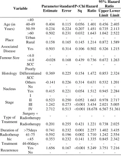
Age (in Years)
<40 - - - -
40-49 0.404 0.115 0.056 1.401 0.456 2.405
50-59 0.234 0.224 0.207 1.451 0.735 2.113
>60 0.502 0.231 0.032 1.643 1.042 2.522
Place Urban - - - -
Rural 0.158 0.165 0.145 1.214 0.872 1.589
Associated
Disease Yes 0.503 0.314 0.106 0.502 0.326 1.215
Tumour Size <4.0 - - - -
>4.0 -0.028 0.168 0.439 0.736 0.672 1.263
Histology
SCC - - - -
Poorly Differentiated
SCC
0.369 0.225 0.154 1.472 0.853 2.324
Others -0.141 0.226 0.314 0.631 0.532 1.201
Nucleus No - - - -
Yes 0.415 0.221 0.054 1.512 0.945 2.284
Stage
I - - - -
II 0.523 0.250 0.052 1.663 0.978 2.717
III 1.242 0.273 <0.001 3.434 2.021 5.005
IV 2.712 0.513 <0.001 18.678 6.567 51.361
Type of Treatment
Surgery +
Radiotherapy - - - -
Radiotherapy 0.201 0.255 0.421 1.221 0.738 2.025
Duration of Radiotherap
hic Treatment
>75days 0.741 0.232 0.001 2.257 1.402 3.435
61-75 0.592 0.196 0.002 1.710 1.242 2.554
<45 0.353 0.232 0.141 1.335 0.845 2.342
46-60days - - - -
Recurrence Yes 1.656 0.167 <0.001 5.249 3.751 7.216
No - - - -
Table 3 Values of -2logL for selected significant models in first step (Analysis I)
Variable -2logL
Value
Difference
Degrees of Freedom
P value
A+N+S+D+R 1617.585 130.443 11 <0.001
A+N+S+D 1711.542 92 - -
A+S+D+R 1643.291 2.21 1 NS
S+R+A+N 1653.361 5.39 1 <0.05
S+R+D+N 1622.819 9.031 1 <0.01
A+N+D+R 1652.932 19.141 1 <0.01
S+R+D+A 1629.695 - - -
S+R+D 1641.702 95.01 1 <0.001
S+R+A 1635.244 5.354 1 <0.05
S+D+A 1614.523 63.645 1 <0.001
R+D+A 1661.178 20.251 1 <0.001
S+R+D+A 1639.846 - - -
S+R+D+Place 1645.561 0.91 1 NS
S+R+D+ Associated
disease 1639.331 0.552 1 NS
S+R+D+
Tumoursize 1635.902 2.956 1 NS
S+R+D+ Histology 1647.276 1.498 1 NS
S+R+D+Type of
Treatment 1631.485 0.012 1 NS
Where
A-Age of the woman N-Change in nucleus S-Stage of the disease
D-Duration of the radio theraphic treatment R-Recurrence during the follow-up period
Table 4 Hazard Ratios from the Cox PH Model (Multi variable Analysis-I)
Variable Paramete
r Estimate Standar d Error
P<Chi. Sq.
Hazard Ratio
95% Confidence
Interval Lower
Limit Upper
Limit
Recurrence 1.346 0.155 <0.001 3.357 3.121 5.181
Duration of Radiotherap
hic Treatment
46-60
days - - - -
≤45 0.363 0.246 0.147 1.431 0.75 2.311
61-75 0.321 0.213 0.052 1.341 0.915 2.131
≥75 0.361 0.242 0.051 1.471 0.871 2.612
Age (in Years)
<40 - - - -
40-49 0.211 0.212 0.506 1.132 0.421 1.631
50-59 0.391 0.140 0.102 1.381 0.826 2.274
≥ 60 0.251 2.340 0.141 1.320 0.760 2.233
Stage of Diseases
I - - - -
II 0.375 0.287 0.154 1.465 0.845 2.525
III 0.871 0.281 0.001 2.532 1.401 4.432
analysis I, again all the five variables recurrence of the disease, duration of radiotherapy treatment, stage of the disease at diagnosis, age of the woman and change in nucleus of the cell have been fitted as explanatory variables. The process of omitting each variable and assessing the significance level of each variable has been done. In Analysis II also, the changes in the nucleus of the cell has been found to be insignificant. Hence, among the remaining four variables, the significance level of each variable has been tested by omitting each variable at a time. The selected four variables are confirmed for their significance. The results are show in table 7.
As in analysis I, all the remaining variables of step I have been entered one by one. No significant contribution has been assessed by the remaining variables. Hence, all the four variables, recurrence of the disease during follow-up, stage of the disease, duration of the radiotheraphic treatement and age of the woman, have been considered for the final model.
As in analysis, I the recurrence of the disease and stage of the disease have been found as significant variables. The other two variables, namely, age of the women and duration of the treatment have been found to be insignificant. This analysis II confirms that omitting of Stage IV patients has not altered the role of the other prognostic variables. The results are show in table 8.
DISCUSSION
Modelling the survival data for prognostic factors in cancer research is on the rise recently in India (Swaminathan, 2002). The main reason is the paucity of follow up information, which is so vital in survival studies. The first and for most assumption of the Cox proportional hazard model is that the censorings are at random. This has been verified. The verification of adequacy of the number of events that are being studied at all levels of factors is desirable. This has been taken care of by suitably classifying the levels of factors in such a way that at each level, there are adequate numbers of events. The stage of the disease has few sample sizes at level IV but proportion of the event is cent percent. Hence, analysis
Table 5 Values of -2 logL for univariate Models (Analysis -II)
Variable -2logL Value
Difference
Degrees of Freedom
P value
Null Model 1618.122 - - -
Age 1603.579 141.512 3 0.002
Place of Residence 1617.261 0.752 1 0.335
Associated Disease 1617.321 0.692 1 0.343
Tumour Size 1611.432 3.562 1 0.53
Histology 1618.056 0.045 1 0.725
Changes in Nucleus 1615.051 3.066 2 0.215
Stage 1629.133 2.780 1 0.084
Type of Treatment 1610.812 26.301 2 <0.001
Duration 1605.036 13.054 3 <0.003
Recurrence 1522.57 87.323 1 <0.001
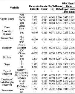
Table 6 Hazard Ratios from the Cox PH Model (Univariate Analysis-II)
Variable Parameter
Estimate
Standard Error
P<Chi Sq
Hazard Ratio
95% Hazard Ratio Upper
Limit Lower
Limit
Age (in Years)
<40 - - - -
40-49 0.372 0.216 0.062 1.380 0.945 2.231
50-59 0.352 0.246 0.130 1.320 0.871 2.242
>60 0.352 0.233 0.050 1.531 0.965 2.503
Place Urban - - - -
Rural 0.150 0.162 0.342 1.172 0.728 1.542
Associated
Disease Yes -0.546 0.326 0.071 0.542 0.251 1.062
Tumour Size <4.0 - - - -
>4.0 -0.056 0.165 0.824 0.954 0.685 1.328
Histology
SCC - - - -
Poorly Different
SCC
0.342 0.274 0.216 1.331 0.521 2.395
Others -0.252 0.224 0.234 0.755 0.466 1.239
Nucleus No - - - -
Yes 0.373 0.221 0.078 1.257 0.732 2.314
Stage
I - - - -
II 0.517 0.260 0.041 1.593 0.967 2.775
III 1.240 0.266 <0.001 3.471 2.021 5.972
Type of Treatment
Surgery +
Radiotherapy - - - -
Radiotherapy 0.226 0.245 0.378 1.271 0.738 2.112
Duration of Radiotheraphic
Treatment
>75days 0.680 0.255 0.378 1.247 0.648 2.112
61-75 0.569 0.198 0.005 1.740 1.175 2.573
<45 0.253 0.249 0.262 1.312 0.691 2.163
46-60days - - - -
Recurrence Yes 1.70 0.179 <0.001 5.416 3.948 7.667
No - - - -
Table 7 Values of -2logL for selected significant models in first step (Analysis II)
Variable -2logL
Value
Difference df P value
R+S+D+A+N 1574.861 - - -
R+S+A+N 1610.141 5.215 1 <0.05
R+S+D+A 1586.932 2.057 1 NS
R+S+D+N 1601.836 7.821 1 <0.01
R+D+A+N 1608.740 13.724 1 <0.001
S+D+A+N 1673.400 67.484 1 <0.001
R+S+D+A 1576.893 - - -
S+D+A 1676.374 68.391 1 <0.001
R+D+A 1612.378 15.355 1 <0.001
R+S+A 1602.006 5.013 1 <0.05
R+S+D 1605.571 8.578 1 <0.01
R+S+D+A 1596.993 - - -
S+R+D+Place 1596.589 0.403 1 NS
S+R+D+Associated disease 1596.032 0.951 1 NS
S+R+D+Type of Treatment 1596.773 0.221 1 NS
S+R+D+ Histology 1595.163 1.73 1 NS
S+R+D+Tumoursize 1594.386 2.601 1 NS
Where
A-Age of the woman N-Change in nucleus S-Stage of the disease
D-Duration of the radio theraphic treatment R-Recurrence during the follow-up period
Table 8 Hazard Ratios from the Cox PH Model (Multi variable Analysis-II)
Variable Parameter
Estimate
Standar d Error
P<Chi. Sq.
Hazard Ratio
95% Confidence
Interval Lower
Limit Upper Limit
Recurrence 1.44 0.175 <0.001 4.765 3.215 6.520
Duration of Radiotheraph ic Treatment
46-60
days - - - -
≤45 0.373 0.251 0.134 1.458 0.857 2.360
61-75 0.357 0.204 0.061 1.331 0.857 2.129
≥75 0.425 0.254 0.078 1.474 0.835 2.523
Age (in Years)
<40 - - - -
40-49 0.121 0.212 0.565 1.120 0.83 1.661
50-59 0.379 0.223 0.108 1.375 0.927 2.365
≥ 60 0.320 0.239 0.216 1.263 0.737 2.119
Stage of Diseases
I 0.363 0.267 0.198 1.423 0.675 2.397
II 0.867 0.238 0.001 2.630 1.395 4.525
II has been performed by omitting stage IV to ascertain the suitability of the Cox-regression model It confirms that the inclusion of the variable stage IV level would not alter the validity of the model The sample size considerations in concern, the overall sample size is 15 per variable. In general, the model with four variables is reliable to make a decision about the prognostic variables of the breast cancer survival. Here, the following four variables have been identified as significant prognostic factors of breast cancer survival for Cox-regression model:
1. Recurrence of the disease 2. Stage of the disease at diagnosis 3. Duration of radiotheraphic treatment 4. Age of the woman at diagnosis
The purpose of applying the Cox-regression is mainly for comparison between the treatment regimens or comparison of dosage level of radiotherapy, their ultimate aim being identification of the prognostic factors of five-year survival probability of breast cancer patients.
Summary
In this Paper, the Cox-regression model building strategy has been discussed. Based on this, two analyses have been done, i.e., with stage IV covariate and without stage IV covariate. Finally, a model with four covariates, namely, recurrence of the disease, age of the woman, duration of radiotheraphic treatment and stage of the disease, has been identified as the prognostic factors of breast cancer survival after the completion of treatment.
Statistical Analysis of Lung Cancer Data
The following sets of data are used for real data examples come from the Veteran’s Administration lung cancer trial, listed in Kalbfleisch and Prentice (1980) and are shown in the Table 2.1. The time variable is survival in days, and the regressors are:
1.
1,
2,
standard
Treatment
test
2.
1,
2,
3,
4,
squamous
small cell
Cell type
adeno
large
3.Karnofsky score: 100-Normal, no evidence of disease
90-Able to carry on normal activity 80-Normal activity with effort
70-Cares for self, unable to carry on normal activity or to do active work
60-Requires occasional assistance but is able to care for most needs
50-Requires considerable assistance and frequent medical care
40-Disabled, requires special care and assistance 30-Severely disabled, hospitalization indicated, although death not imminent
20-Very sick, hospitalization necessary 10-Moribund, fatal process progressing rapidly 0-Dead
1. Months from diagnosis. 2. Age in years.
3.
0,
1,
no
Prior therapy
yes
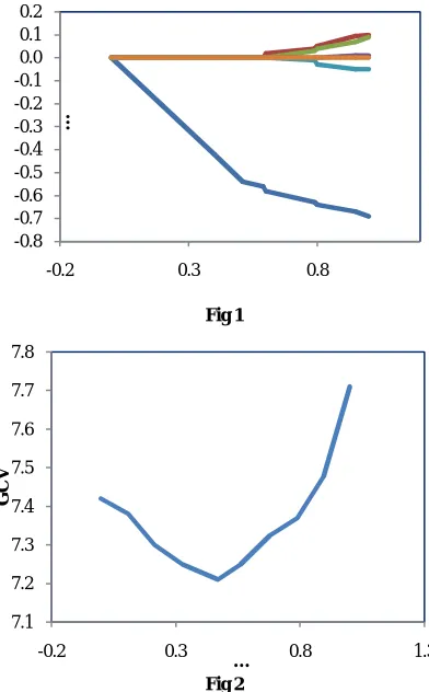
For simplicity and the categories exhibit increasing risk, cell type as a numerical variable. A standard proportional hazards analysis shows that the Karnofsky score is extremely important, while cell type is also strongly significant. The estimated coefficients from the LASSO fit as a function of the standardized constraint parameter
0
j
s
u
where j0 are the unconstrained partial likelihood estimates.
The value of u chosen by Generalized Cross-Validation (GCV) statistics suggested by Wahba (1980). To construct this statistic, we need a linear approximation to the LASSO
estimate. We write the constraint ∑ ≤ as ∑ ≤ .
This latter constraint is equivalent to adding a Lagrangian penalty ∑ to the log partial likelihood, with 0 depending on s. Intuitively, these are equivalent since they both lead to a balance between fit, as measured by the log partial likelihood, and the value of ∑ . Using standard matrix manipulations, we may write the constrained solution in step 3 in the form
1β
T TX DX
W
X Dz
… (7)
where, W = diag(Wj),
1 /
0
0
j j
i
if
W
otherwise
… (8)
This expression does not give a numerically effective way of computing the LASSO estimate, but it is useful for assessing the complexity of the fit. Therefore we may approximate the number of effective parameters in the constrained fit by
T
1 Tp s
tr X X DX
W
X D
Letting ‘ls’ be the log-partial likelihood for the constrained fit
with constraint s, we construct the GCV statistic
21
1
/
s
l
GCV s
N N
p s
N
… (9)Use approximation of equ. (7) to yield an approximate method for obtaining standard errors for the LASSO estimates. In the notation of equ. (7), using standard partial likelihood theory that the variance of z is approximately D-1. Letting M denote the matrix that multiplies z in equ. (7), then the variance of = is approximately MD-1MT. Hence we can obtain the approximate standard errors of from the square root of the diagonal of MD-1MT. The resulting coefficient estimates for backward stepwise selection in the standard Cox model yields the same single variable model, but with a coefficient of -0.56 (0.10) or a relative risk 0.55. The stepwise method refers to backward-forward stepwise selection as implemented in Scott Emerson’s S language function ‘coxrgrss’ with the default P-values to enter and remove of 0.05 and 0.10, respectively. Schwarz’s criterions also known as BIC to these data, this has the form minus log partial likelihood plus ‘k log(n)’ where k is the number of regressors in the model considered and n is the sample size. Searching over all subsets, the model that minimizes Schwarz’s criterion again contained only the Karnofsky score. Coefficient estimates for lung cancer example, as a function of the standardized constraint parameter
u
s
/
|
0j| .
The generalized cross-validation score is plotted against the standardized constraint parameter
u
s
/
|
0j| .
using GCV plot is given in Fig. 1 and Fig. 2. For a detailed study refer to Wahba (1980).A Simulation Study
180 datasets each with 50 observations has been simulated from the exponential hazard model
t x
|
exp
Tx
… (10)where = (-0.33, -0.33, 0, 0, 0, -0.33, 0, 0, 0)T.
The xi were each marginally standard normal, and the
correlation between xi and xj was |i-j| with = 0.5 and gave
moderate to strong effects for the three regressors with
non-zero coefficients. Letting Σ be the population covariance
matrix of the regressors. To investigate the accuracy of the
procedure, with βj = 0.1 for all j and the median of the mean
squared errors
T
β β
β β
over 100 simulations forthe model in equ. (10) and the results were shown in table 10, table 11 and table 12.
Fig 1
Fig 2
-0.8 -0.7 -0.6 -0.5 -0.4 -0.3 -0.2 -0.1 0.0 0.1 0.2
-0.2 0.3 0.8
…
7.1 7.2 7.3 7.4 7.5 7.6 7.7 7.8
-0.2 0.3 0.8 1.3
G
C
V
…
Table 9 Lung Cancer Data*
Tr CT t x1 x2 x3 x4
1 1 71 60 7 68 0
1 1 410 71 4 62 10
1 1 225 62 3 35 0
1 1 125 62 9 62 10
1 1 119 68 11 63 10
1 1 10 19 5 48 0
1 1 81 40 10 68 10
1 1 111 81 28 69 0
1 1 315 50 16 42 0
1 1 100 78 5 70 0
1 1 43 62 4 80 0
1 1 8 39 57 62 10
1 1 145 30 4 64 0
1 1 26 81 9 54 10
1 1 11 70 11 48 11
1 2 30 60 3 62 0
1 2 383 61 9 44 0
1 2 3 41 2 34 0
1 2 54 80 4 63 10
1 2 13 61 4 55 0
1 2 123 41 3 56 0
1 2 97 60 5 68 0
1 2 154 60 14 62 10
1 2 60 30 2 65 0
1 2 117 80 3 46 0
1 2 16 30 4 53 10
1 2 151 50 12 69 0
1 2 22 60 4 67 0
1 2 56 80 12 42 10
1 2 21 40 2 54 10
1 2 18 20 15 41 0
1 2 139 80 2 63 0
1 2 20 31 5 66 0
1 2 31 74 3 65 0
1 2 51 71 2 55 0
1 2 286 60 25 66 10
1 2 18 30 4 60 0
1 2 51 60 1 67 0
1 2 122 80 28 53 0
1 2 27 60 8 62 0
1 2 54 70 1 67 0
1 2 7 50 7 72 0
1 2 63 50 11 48 0
1 2 392 40 4 68 0
1 2 10 40 23 67 10
1 3 8 20 19 61 10
1 3 92 70 10 60 0
1 3 35 40 6 62 0
1 3 117 80 2 38 0
1 3 132 80 5 50 0
1 3 12 50 4 63 10
1 3 162 80 5 64 0
1 3 3 30 3 43 0
1 3 95 80 4 34 0
1 4 177 50 16 66 10
1 4 162 80 5 62 0
1 4 216 50 15 52 0
1 4 553 70 2 47 0
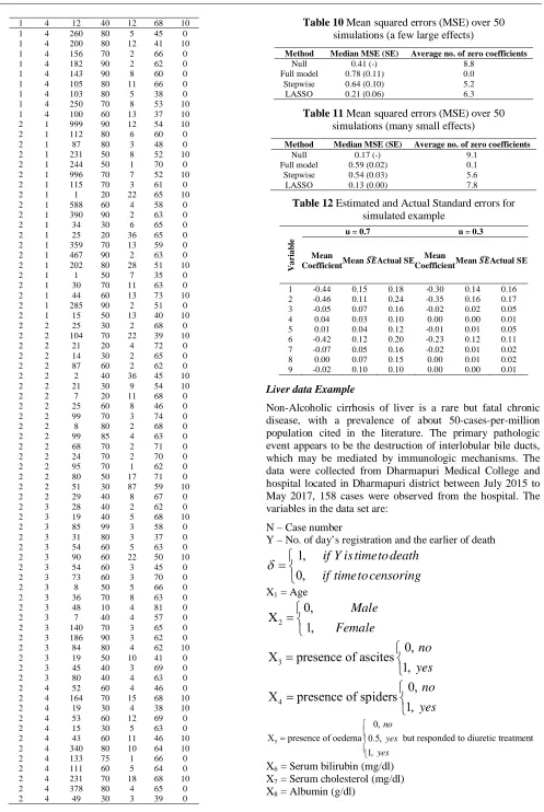
Liver data Example
Non-Alcoholic cirrhosis of liver is a rare but fatal chronic disease, with a prevalence of about 50-cases-per-million population cited in the literature. The primary pathologic event appears to be the destruction of interlobular bile ducts, which may be mediated by immunologic mechanisms. The data were collected from Dharmapuri Medical College and hospital located in Dharmapuri district between July 2015 to May 2017, 158 cases were observed from the hospital. The variables in the data set are:
N – Case number
Y – No. of day’s registration and the earlier of death
1,
0,
if Y is timeto death
if timeto censoring
X1 = Age
2
0,
X
1,
Male
Female
3
0,
X
presence of ascites
1,
no
yes
4
0,
X
presence of spiders
1,
no
yes
5
0,
X presence of oedema 0.5, but responded to diuretic treatment
1,
no yes yes
X6 = Serum bilirubin (mg/dl)
X7 = Serum cholesterol (mg/dl)
X8 = Albumin (g/dl)
1 4 12 40 12 68 10
1 4 260 80 5 45 0
1 4 200 80 12 41 10
1 4 156 70 2 66 0
1 4 182 90 2 62 0
1 4 143 90 8 60 0
1 4 105 80 11 66 0
1 4 103 80 5 38 0
1 4 250 70 8 53 10
1 4 100 60 13 37 10
2 1 999 90 12 54 10
2 1 112 80 6 60 0
2 1 87 80 3 48 0
2 1 231 50 8 52 10
2 1 244 50 1 70 0
2 1 996 70 7 52 10
2 1 115 70 3 61 0
2 1 1 20 22 65 10
2 1 588 60 4 58 0
2 1 390 90 2 63 0
2 1 34 30 6 65 0
2 1 25 20 36 65 0
2 1 359 70 13 59 0
2 1 467 90 2 63 0
2 1 202 80 28 51 10
2 1 1 50 7 35 0
2 1 30 70 11 63 0
2 1 44 60 13 73 10
2 1 285 90 2 51 0
2 1 15 50 13 40 10
2 2 25 30 2 68 0
2 2 104 70 22 39 10
2 2 21 20 4 72 0
2 2 14 30 2 65 0
2 2 87 60 2 62 0
2 2 2 40 36 45 10
2 2 21 30 9 54 10
2 2 7 20 11 68 0
2 2 25 60 8 46 0
2 2 99 70 3 74 0
2 2 8 80 2 68 0
2 2 99 85 4 63 0
2 2 68 70 2 71 0
2 2 24 70 2 70 0
2 2 95 70 1 62 0
2 2 80 50 17 71 0
2 2 51 30 87 59 10
2 2 29 40 8 67 0
2 3 28 40 2 62 0
2 3 19 40 5 68 10
2 3 85 99 3 58 0
2 3 31 80 3 37 0
2 3 54 60 5 63 0
2 3 90 60 22 50 10
2 3 54 60 3 45 0
2 3 73 60 3 70 0
2 3 8 50 5 66 0
2 3 36 70 8 63 0
2 3 48 10 4 81 0
2 3 7 40 4 57 0
2 3 140 70 3 65 0
2 3 186 90 3 62 0
2 3 84 80 4 62 10
2 3 19 50 10 41 0
2 3 45 40 3 69 0
2 3 80 40 4 63 0
2 4 52 60 4 46 0
2 4 164 70 15 68 10
2 4 19 30 4 38 10
2 4 53 60 12 69 0
2 4 15 30 5 63 0
2 4 43 60 11 46 10
2 4 340 80 10 64 10
2 4 133 75 1 66 0
2 4 111 60 5 64 0
2 4 231 70 18 68 10
2 4 378 80 4 65 0
2 4 49 30 3 39 0
Table 10 Mean squared errors (MSE) over 50 simulations (a few large effects)
Method Median MSE (SE) Average no. of zero coefficients
Null 0.41 (-) 8.8
Full model 0.78 (0.11) 0.0
Stepwise 0.64 (0.10) 5.2
LASSO 0.21 (0.06) 6.3
Table 11 Mean squared errors (MSE) over 50 simulations (many small effects)
Method Median MSE (SE) Average no. of zero coefficients
Null 0.17 (-) 9.1
Full model 0.59 (0.02) 0.1
Stepwise 0.54 (0.03) 5.6
LASSO 0.13 (0.00) 7.8
Table 12 Estimated and Actual Standard errors for simulated example
V
a
r
ia
b
le
u = 0.7 u = 0.3
Mean
Coefficient Mean Actual SE Mean
Coefficient Mean Actual SE
1 -0.44 0.15 0.18 -0.30 0.14 0.16
2 -0.46 0.11 0.24 -0.35 0.16 0.17
3 -0.05 0.07 0.16 -0.02 0.02 0.05
4 0.04 0.03 0.10 0.00 0.00 0.01
5 0.01 0.04 0.12 -0.01 0.01 0.05
6 -0.42 0.12 0.20 -0.23 0.12 0.11
7 -0.07 0.05 0.16 -0.02 0.01 0.02
8 0.00 0.07 0.15 0.00 0.01 0.02
5160
X9 = Alkaline phosphate (IU/liter)
X10 = SGOT (IU/ml)
X11 = Triglycerides (mg/dl)
X12 = Platelet count; coded value is number of platelets per
cubic meter (mg/dl)
X13 = Prothrombin time (in sec.)
X14 = Histological state of disease, graded 1, 2, 3 or 4.
The result appears in table 5.5, for the full model, stepwise and LASSO. The stepwise method is implemented for using the Scott Emerson’s S language function ‘coxgrss’ (refer to the website: lib.stat.cmu.edu). the model is fitted with 14 variables.
The estimated regression coefficients together with GCV statistics is computed from equ. (7) and equ. (8). The standard error for the LASSO estimates can be obtained by using the approximately given in the equ. (7). The approximation can be done using standard partial likelihood theory that the variance of z is approximately D-1. Letting M denote the matrix that multiplies z in equ. (7), then the variance of
= is approximately MD-1MT. Hence we can obtain the approximate standard errors of from the square root of the diagonal of MD-1MT. For data simulation, the procedure given in section 2 can be used. From the table 10, table 11 and table 12; the LASSO outperforms the full and stepwise models by shrinking the coefficients almost all of the way to zero. From the analysis of liver data shown in table 13, the GCV procedure gave = 0.59 for the standardized LASSO parameter and the resulting model from the lasso looks similar to the stepwise model and full model.
The LASSO technique for variable selection in the Cox model seems a worthy competitor to stepwise selection. It is less variable than the stepwise approach and still yields interpretable models. The LASSO method requires initial standardization of the regressors, so that the penalization scheme is fair to all regressors. The LASSO clearly outperforms stepwise selection, and picks approximately the correct number of zero coefficients. The proposed methodology cited in this paper has focused on fixed covariates analysis. But one can incorporate time dependent covariate without any new difficulty.
CONCLUSION
In this Paper, Semi and non semi parametric models for reliability analysis has been discussed
.
Based on this, the analyses has been carried out. Further it is evident that, a model with four covariates, namely, recurrence of the disease, age of the woman, duration of radiotheraphic treatment and stage of the disease, has been identified as the prognostic factors of breast cancer survival after the completion of treatment.Reference
1. Breslow, N. (1975). Analysis of survival data under the proportional hazards model. Int. Statist. Rev., 43, 45-57.
2. Bunea, F. and McKeague, I.W. (2005). Covariate Selection for Semiparametric Hazard Function Regression Models. Jour. of Multivariate Analysis, 92, 186-204
3. Fan, J. and Li, R. (2002). Variable Selection for Cox’s Proportional Hazards Model and Frailty Model. The Anns. of Stat., 30(1), 74-99.
4. Finkelstein, D.M. (1986). A Proportional Hazards Model for Interval-Censored Failure Time Data.
Biometrics, 42, 845-854.
5. Androulakis, E., Koukouvinos, C., Mylona, K. and Vonta, F. (2010), A real survival analysis application via variable selection methods for Cox´s proportional hazards model, Journal of Applied Statistics ,47, No 8, 1399-1406
Table 13 Results for Liver data
Variables
Full Stepwise LASSO
Co- efficient SE
Z- score
Co- efficient SE
Z- score
Co- efficient SE
Z- Score
1 0.27 0.13 2.41 0.30 0.08 3.11 0.18 0.80 1.80
2 -0.13 0.10 -0.11 - - - -0.02 0.01 -0.31
3 0.02 0.11 0.20 - - - 0.02 0.07 0.53
4 0.06 0.10 0.43 - - - 0.03 0.04 0.36
5 0.28 0.11 2.56 0.20 0.06 3.50 0.12 0.10 1.56
6 0.31 0.12 3.20 0.32 0.06 4.20 0.30 0.12 2.81
7 0.11 0.11 1.05 - - - 0.01 0.02 0.25
8 -0.30 0.12 -2.45 -0.24 0.10 -2.51 -0.30 0.12 -2.30
9 0.00 0.09 0.02 - - - 0.00 0.00 0.00
10 0.24 0.10 2.17 0.22 0.11 2.29 0.10 0.09 1.09
11 -0.08 0.06 -0.70 - - - 0.01 0.00 0.00
12 0.07 0.11 0.70 - - - 0.01 0.00 0.00
13 0.21 0.11 2.10 0.20 0.14 2.35 0.07 0.12 1.02
14 0.35 0.13 2.61 0.35 0.16 3.05 0.21 0.08 2.34
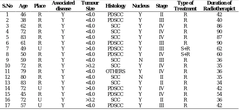
Appendix
S.No Age Place Associated disease
Tumour
Size Histology Nucleus Stage
Type of Treatment
Duration of Radiotherapict
1 46 R Y <4.0 PDSCC Y II R 42
2 38 R Y <4.0 PDSCC Y III R 40
3 62 R Y <4.0 SCC Y IV R 86
4 72 R Y <4.0 SCC Y IV R 90
5 83 R Y <4.0 SCC Y IV R 87
6 61 R Y <4.0 PDSCC Y III R 90
7 49 U Y >4.0 PDSCC Y III S+R 62
8 50 R Y <4.0 PDSCC Y IV S+R 60
9 59 R Y <4.0 SCC N III R 36
10 72 R Y >3.2 SCC Y IV R 35
11 79 R Y <4.0 OTHERS Y IV R 36
12 80 R Y <4.0 SCC N II R 35
13 83 R Y <4.0 SCC Y II R 34
14 72 U Y >4.0 PDSCC Y IV R 42
15 45 R Y <4.0 PDSCC Y IV R 54
16 72 U Y >3.2 SCC Y II R 36
5161
Appendix
S.No Age Place Associated disease
Tumour
Size Histology Nucleus Stage
Type of Treatment
Duration of Radiotherapict
18 58 U Y <4.0 PDSCC Y III R 40
19 60 U Y <4.0 OTHERS Y III S+R 46
20 59 R Y <4.0 SCC Y II R 52
21 72 R Y >4.0 SCC Y IV R 59
22 48 R Y >4.0 OTHERS Y III R 63
23 53 R Y <4.0 SCC Y IV R 60
24 57 R Y <4.0 OTHER Y IV R 63
25 69 R Y <4.0 OTHER Y IV R 55
26 67 R N <4.0 SCC Y III R 45
27 63 R Y >4.0 OTHER Y I R 76
28 52 U Y >4.0 SCC Y II R 79
29 45 R Y <4.0 SCC Y IV R 33
30 39 U Y <4.0 OTHER Y IV R 40
31 42 U Y <4.0 SCC Y IV R 29
32 40 R Y <4.0 SCC Y III R 26
33 32 R Y <4.0 SCC Y II R 37
34 59 U Y <4.0 OTHER Y III R+S 22
35 58 R Y <4.0 OTHER Y II R 32
36 61 R Y <4.0 OTHER Y III R 45
37 69 R Y >4.0 SCC Y II R 67
38 67 R Y <4.0 SCC Y III R 56
39 55 R Y <4.0 SCC Y II R 43
40 46 R Y <4.0 OTHER Y III R 55
41 56 R Y <4.0 SCC Y IV R 35
42 46 R Y <4.0 PDSCC Y II R 42
43 38 R Y <4.0 PDSCC Y III R 40
44 62 R Y <4.0 SCC Y IV R 86
45 72 R Y <4.0 SCC Y IV R 90
46 83 R Y <4.0 SCC Y IV R 87
47 61 R Y <4.0 PDSCC Y III R 90
48 49 U Y >4.0 PDSCC Y III S+R 62
49 50 R Y <4.0 PDSCC Y IV S+R 60
50 59 R Y <4.0 SCC N III R 36
51 72 R Y >3.2 SCC Y IV R 35
52 79 R Y <4.0 OTHERS Y IV R 36
53 80 R Y <4.0 SCC N II R 35
54 83 R Y <4.0 SCC Y II R 34
55 72 U Y >4.0 PDSCC Y IV R 42
56 45 R Y <4.0 PDSCC Y IV R 54
57 72 U Y >3.2 SCC Y II R 36
58 57 U Y <4.0 PDSCC Y III R 42
59 58 U Y <4.0 PDSCC Y III R 40
60 60 U Y <4.0 OTHERS Y III S+R 46
61 59 R Y <4.0 SCC Y II R 52
62 72 R Y >4.0 SCC Y IV R 59
63 48 R Y >4.0 OTHERS Y III R 63
64 53 R Y <4.0 SCC Y IV R 60
65 57 R Y <4.0 OTHER Y IV R 63
66 69 R Y <4.0 OTHER Y IV R 55
67 59 U Y <4.0 OTHER Y III R+S 22
68 58 R Y <4.0 OTHER Y II R 32
69 61 R Y <4.0 OTHER Y III R 45
70 69 R Y >4.0 SCC Y II R 67
71 67 R Y <4.0 SCC Y III R 56
72 55 R Y <4.0 SCC Y II R 43
73 46 R Y <4.0 OTHER Y III R 55
74 56 R Y <4.0 SCC Y IV R 35
75 50 R Y <4.0 OTHER Y II R 45
76 45 R Y <4.0 SCC Y II R 39
77 59 R Y <4.0 OTHER Y III R 27
78 63 R Y <4.0 SCC Y II R 65
79 34 R Y <4.0 OTHER Y III R 55
80 30 U Y >4.0 SCC Y II R 50
81 45 R Y <4.0 SCC Y II R 65
82 54 R Y <4.0 SCC Y III R 60
83 59 U Y <4.0 SCC Y IV R 54
84 67 R N <4.0 SCC Y III R 45
85 63 R Y >4.0 OTHER Y I R 76
86 52 U Y >4.0 SCC Y II R 79
87 45 R Y <4.0 SCC Y IV R 33
88 39 U Y <4.0 OTHER Y IV R 40
89 42 U Y <4.0 SCC Y IV R 29
90 40 R Y <4.0 SCC Y III R 26
91 32 R Y <4.0 SCC Y II R 37
92 72 R Y >3.2 SCC Y IV R 35
93 79 R Y <4.0 OTHERS Y IV R 36
94 80 R Y <4.0 SCC N II R 35
95 83 R Y <4.0 SCC Y II R 34
96 72 U Y >4.0 PDSCC Y IV R 42
97 45 R Y <4.0 PDSCC Y IV R 54
98 72 U Y >3.2 SCC Y II R 36
99 57 U Y <4.0 PDSCC Y III R 42