Abstract—Preparations for possible disasters should be made to minimize the damage caused by events such as fires and earthquakes. Several kinds of disaster simulations have been developed for this reason. Many evacuation simulation methods are based on multi-agent systems. These are considered to be useful and powerful methods of dealing with complex systems containing several elements, and have been proposed for safely guiding evacuees. The social force model is one approach that considers the influences and interactions between evacuees. When aiming to improve the precision of social force model simulations, the model parameters should be appropriately determined. In this paper, a method for determining the parameters used in the social force model is proposed by applying an evolutionary computing method to collect evacuee flow data.
Index Terms—Evacuation simulation, social force model, pedestrian model, genetic algorithm.
I. INTRODUCTION
To ensure the structural reliability and safety of architecture, not only should structural performance be considered during events such as earthquakes, but also other elements of the system such as software and human occupants. In recent years, buildings have been designed with multiple floors and with greater underground area with the aim of using urban space more efficiently. However, as a result of this, evacuation from buildings with more complicated layouts can take more time in the event of a disaster. A range of options have been discussed to reduce the danger posed by disasters from various viewpoints. It is thought that huge disasters in tectonically unstable areas, such as the Nankai Trough in the south of Japan, will occur with a high probability in near future. Therefore, preparatory planning for large natural disasters is an urgent and important issue.
Considering the many victims of disasters such as fires and earthquakes that have already occurred, the importance of evacuation countermeasures has been highlighted in addition to that of structural building resilience. Computer simulations are powerful and efficient tools for estimating the temporal and spatial patterns of events that occur during a disaster, a many simulation models of pedestrian behavior have been proposed to identify the laws underlying crowd dynamics and to predict the level of danger and confusion that occurs during s evacuation [1]–[6]. In addition, these evacuation simulation are carried out at the building design stage with the aim of
Manuscript received November 5, 2018; revised May 2, 2019. This work was supported by JSPS KAKENHI Grant Number 16K01295.
T. Miyoshi is with Hannan University, Osaka, 558-8502, Japan (e-mail: [email protected]).
improving evacuation efficiency of, for example, underground shopping areas.
Several kinds of disaster simulations have been developed to determine the effect of damage using assumed situations such as influence of smoke and passage blockage. In particular, evacuation simulation methods using multi-agent systems have been proposed for guiding evacuees, in which multiple evacuees are represented using autonomous agents, and the temporal and spatial dynamics of evacuation are estimated by the simulation. The social force model is one evacuation simulation model that considers the influence of multiple evacuees [2], [4], [5].
It is pointed out that there is no International standard on the methods and tests to assess the verification and validation (V&V) of building fire evacuation models and the uncertainties associated with evacuation modelling are discussed [7]. Some methods to decide a set of parameters appropriately have been proposed to guarantee the accuracy and reliability of the simulation results. Johansson et al. have proposed an evolutionary optimization algorithm to determine optimal parameter specifications for the social force model using the suitable video recordings of interactive pedestrian [8]. Nonaka et al. have proposed a walking velocity model for accurate pedestrian simulations, in which presents the relation between pedestrian density and velocity distribution that was generated through analyzing flows observed from actual pedestrian movement in evacuation [9]. In aiming to improve the precision of the simulation, the parameters included in this model should be appropriately determined.
In this paper, we propose a method for determining the parameters of the social force evacuation model using the evolutionary computation. The method is used to represent the flow of evacuees during an emergency, which is evaluated through a comparison with actual evacuees. For this purpose, we carried out several experiments to gather flow data for real subjects under several walking conditions and applied the proposed method to determine the parameters of the model from the flow data. We discuss the performance of the method and compare group flow dynamics in the experiments with corresponding real-life evacuation simulations.
Section II summarizes the construction method of the evacuation simulation. In Section III, we summarize the experimental methods used for the model evaluation, and summarize the experimental results in Section IV. In Section V, we propose a method for estimating the parameters of the simulation model from the measurement data using an evolutionary computation algorithm, and we evaluate the estimation result. Finally, Section VI summarizes the key findings of the research.
Identification of Parameters for a Social Force Model in
Evacuation Simulation Using Evolutionary Computation
Target
1
2
3
4
i
fi1Counterforce
fi4
fi3
Friction
fi4
Counterforce
fiw
i
Friction
fiw
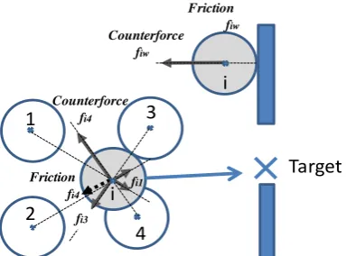
Fig. 1. Forces acting on each agent from the model configuration.
(a) Single direction (b) Opposite direction Fig. 2. Configuration of walking experiments.
II. EVACUATION SIMULATION MODEL
A. Experiment Configuration
Firstly, this section describes a model for carrying out the evacuation simulation, in which evacuees are represented by autonomous and interrelated agents. The original dynamic model of the agents is defined by assuming a range of socio-psychological and physical forces that influence crowd behavior according to the literature [2]. In crowds, pedestrians’ movements depend on various external influences and internal motivations. In this model, agents tend to keep a velocity-dependent distance from other agents, walls, and other obstructions such as display shelves and desks, and these repulsive forces are defined as the interaction forces between elements [2]:
𝑚𝑖
d𝒗𝑖
d𝑡 =𝑚𝑖
𝒗𝑖0 𝑡 𝑒𝑖0 𝑡 − 𝒗𝑖 𝑡
𝜏𝑖
+ 𝒇𝑖𝑗
𝑗 ≠𝑖
+ 𝒇𝑖𝑤
𝑤
+ 𝒇𝑖𝑜
o (1) where mi is the mass of agents, v0
i is a certain desired velocity
and vi(t) is a current velocity vector of agent I, respectively,
and e0
i is a desired direction vector. The second term in Eq.
(1) is the applied force, defined from the repulsive force and the frictional force acting between agents I and j, which is called the interaction force fij. The third term fiw represents the reaction force from the walls (see Fig. 1).
During an evacuation, evacuees interact with each other; they keep a distance (personal space) and furthermore they may be pushed by others when they are stranded in closed range. Thus, agent I in the evacuation simulation experiences several interaction forces from agent j,as follows:
𝑓𝑖𝑗 = 𝑎1𝑖 exp 𝑟𝑖𝑗− 𝑑𝑖𝑗
𝑏1𝑖
+𝑘𝑔 𝑟𝑖𝑗− 𝑑𝑖𝑗 𝒏𝑖𝑗
+𝑢𝑔 𝑟𝑖𝑗 − 𝑑𝑖𝑗 ∆𝑣𝑖𝑗𝑡 𝒕𝑖𝑗 (2)
The total interaction force from other agents can be summarized as the second term in Eq. (1).
In calculating the reaction force from walls and obstacles (expressed by the third term of Eq. (1)), several nodes are set on walls and obstacles at intervals that are smaller than the size of the agent. Then, the magnitude of the applied force to the agent was determined by the positional relationship of the nearest neighbor node to the agent. The reaction force from the wall [2]was defined as follow:
𝑓𝑖𝑤= 𝑎2𝑖 exp
𝑟𝑖𝑤− 𝑑𝑖𝑤
𝑏2𝑖
𝑘𝑔 𝑟𝑖𝑤− 𝑑𝑖𝑤 𝒏𝑖𝑤
+𝑢𝑔 𝑟𝑖𝑤− 𝑑𝑖𝑤 ∆𝑣𝑖𝑤𝑡 𝒕𝑖𝑤 (3)
The time sequence of the flow of agents was defined by the dynamic system of Eq. (1), Eq. (2), and Eq. (3), which depended on the parameters in the model.
III. MEASUREMENT OF PEDESTRIAN FLOW
A. Procedure of Experiments
In this research, the two kinds of experiments were carried out to measure the flow of real subjects to generate the dataset from which the model parameters were estimated. The first experiment was conducted to specify the walking speed of the subjects. For this, all subjects were asked to walk in a clockwise direction along a passage in a lecture room, as shown as Fig. 2. The width of the passage was 1 m. In the second experiment, half of subjects walked in a clockwise direction and the other half walked in an anti-clockwise direction, using the same room configuration as the first experiment. We recorded the flow of the subjects in both experiments using a 360-degree omnidirectional camera (SP 360, Kodak Ltd.). As the subjects walked in opposite directions in the second experiment, they sometimes met and, as a result, walked with stronger interaction force than subjects in the first experiment.
B. Condition of Agent Movement
In each experiment, to control the speed at which each subject moved, we played a double-beat sound using metronome. According to [6], it is reported that a correlation is generally observed between the speed of played sound and the walking speed of healthy listeners; in the case of 100 steps per minutes, walking speed is approximately 4 km per hour. In this research, it was assumed that during an emergency evacuation, walking speed would be much faster; experiments were carried out by setting the metronome at three different speeds: (1) 120 steps per min; (2) 150 steps per min; and (3) 180 steps per min. In addition, even if congestion occurred (due to an evacuation route becoming a bottleneck, for example). We ensured that the walking pace of the subjects was maintained relatively constant.
C. Subjects
experimental procedure to the subjects, and their approval to take part was then confirmed.
D. Experimental Configuration
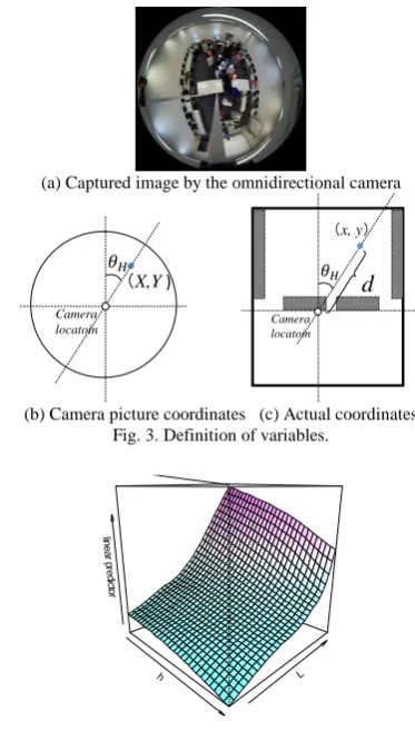
The flow of subjects along the passage were recorded under the different walking speeds. From this video stream, we captured images and computed the positions of the subjects in the room during the experiments using the convenient method of calculating physical coordinates. A sample captured image from the video recording is shown in Fig. 3(a).
Fig. 3(b) indicates a subject’s spatial position (X, Y) and angle (θH) relative to a line of origin from the position of the video camera. The position of the subject (x, y) in the room as computed from the image is indicated in Fig. 3(c). However, the coordinate position of a subject on the floor could not be directly estimated from the captured images because the subjects’ legs were obscured. The recorded positions in the images (X, Y) therefore reflected the tops of the subject’s heads and actual standing positions were calculated based on subject height.
Prior to the evacuation gait experiment, in order to specify the numerical relationship among the pixel coordinates (X, Y) on the camera images, the heights of the subjects, and the room position coordinates (x, y), the spatial coordinates of sampling points in the physical experimental were gathered. These coordinates consisted of horizontal and vertical coordinates representing the position in the room and height within the physical space. Specifically, we select the sampling points at every 0.5 m above the radiation centering on the position of the camera and measured the pixel coordinates (X,
Y) at the every 0.1m vertical height. Due to the physical limitations of the experiment space, the number of measurement points was 170. The mapping function from both the camera coordinates and the coordinates for the vertical upper from the floor were obtained by nonlinear regression based on the gathered dataset. The obtained mapping function is shown in Fig. 4. The error in the coordinates for the experiment space as converted by this mapping function was 1.03% on average. In the 360-degree omnidirectional images, each study object was radially taken from the center of the camera, but the shooting distortion to the depth was close to zero by the radiation angle θH.
IV. RESULT OF EXPERIMENT
A. Result of the First Experiment
In the first experiment, the subjects were instructed to walk all in a clockwise direction at a pace of 120, 150, and 180 steps per minute. The flow of subjects walking along the passage was recorded and images were then captured at each 500 ms intervals from the video stream. The positions of subjects were specified on the captured image and the position of the real environment was calculated by the method described in Section III D. Fig. 5 shows the movement trajectory of subject 1 under the first speed condition (120 steps per minute) and the third condition (180 steps per minute). The origin for the room coordinates was set to the bottom left point as shown in Fig. 2. The average velocities of five subjects randomly selected for speed conditions 1 and 3 were 0.91 m/s and 1.02 m/s, respectively. Nevertheless the
subjects were instructed to keep walking pace, the averages of velocities with two conditions are different from the expected value. This result is because there was a strong tendency to keep a certain distance between the subjects, and when the length of the row became long, the first subject followed the last subject of the row. In these cases, walking pace was restricted and the subjects could not walk at the designated pace.
(a) Captured image by the omnidirectional camera
(X,Y )
Camera locatoin
(x, y)
d
Camera locatoin
(b) Camera picture coordinates (c) Actual coordinates Fig. 3. Definition of variables.
h L
line
a
r p re dic to
r
Fig. 4. Relationship between captured distance on the experimental pictures and actual distance.
a) Speed configuration 1 b) Speed configuration 3 (120 steps/s) (180 steps/s)
Fig. 5. Trajectory of subject 1 during Experiment 1 (sampling time was 500 ms).
-70
0
-60
0
-50
0
-40
0
-30
0
-20
0
-10
0
0
1
0
0
2
0
0 -20
0
0
2
0
0
4
0
0
-70
0
-60
0
-50
0
-40
0
-30
0
-20
0
-10
0
0
1
0
0
2
0
0 -20
0
0
2
0
0
4
0
0
0 2 4 6 8(m) 6
4
2
6
4
2
0 2 4 6 8(m)
Fig. 6. Trajectory of subject 1 and 2 during Experiment 2 (sampling time is 500 ms).
B. Result of Second Experiment
other 14 subjects walking in an anti-clockwise direction. The subjects were instructed to walk on the left-hand side of the passage. Therefore, the subjects walking in the clockwise direct walked on the inside of the passage and the others walked on the outside. Fig. 6 shows the movement trajectories of subject 1 and subject 2 under velocity condition 1. It can be seen from this figure that the subjects walked on the left side of passage as instructed. The average speed by speed condition was 1.01 m/s and 1.33 m/s, and the average speed is the ratio of the number of steps. Since the number of subjects in both groups was not large (unlike the first experiment), the subjects could maintain their walking speed.
V. ESTIMATION OF AGENT MODEL PARAMETERS USING EC
A. Procedure of Parameter Estimation Using EC
The simulation model consists of the following parameters: the target speed used in the evacuee model; the reaction force and the frictional force acting between the agents; the reaction force with fixtures such as a wall; and the frictional force used the evacuee model. All of these parameters need to be set correctly. In order to express the flow of subjects in the experiments using the simulation model (as calculated from the captured images described in the previous section), appropriate parameters should be included in the agent model.
We describe the estimation procedure for parameters included in the evacuee model from measured agent flow data. Considering the differences in personal characteristics such as sex, age, and physical characteristics of agents in general, the parameters included in the evacuee model are not homogeneous but vary. In the evacuation simulations, it is difficult to optimize each parameter at the same time since the position of an agent is determined as the time integration of the evacuee model with the interaction among evacuees. Therefore, considering that evacuation models are represented by combinations of individual parameters for multiple agents, the determination of appropriate parameters is a problem involving the approximation of human flow data.
B. Evaluation Function and Genetic Structure in
Evolutionary Optimization
Assuming that I is the number of agents included in the simulation, the actual measured position and the position in the simulation at time t of agent i(i = 1,...,I) is xe
i(t) = (xe1i(t), xe
2i(t)) and xs1i(t) = (xs1i(t), xs2i(t)), respectively. The average
distance of each agent (at each time step) between the experimental data and the simulated data is defined as an index of appropriateness of the parameters (I.A.):
𝐸= 𝒙𝑖𝑠 𝑗∆𝑡 − 𝒙 𝑖 𝑒 𝑗∆𝑡 𝐽
𝑗 𝐼
𝑖
(4) In calculating I.A., however, both the measured position of the agent and the position in the simulation were discretized into errors for each sampling time Δt and tabulated. The distance between two points was defined with the Euclidean norm. J represents the sampling number at this time. The I.A. value calculated using Eq. (4) indicates the degree of
conformity of the evacuation simulation to the actual data; the smaller the evaluation function value, the better the simulation model was parameterized to represent the experimental flow data.
TABLE I: PARAMETER VALUES
Parameter Values
v0 Integer from 7 to 23
a1 50, 100, 200, 300, 400, 500, 600, 700, 800
b1 0.2, 0.3, 0.4,0.5,0.6,0.7
a2 50, 100, 200, 300, 400, 500, 600, 700, 800
b2 0.2, 0.3, 0.4, 0.5, 0.6, 0.7
TABLE II: MINIMUM VALUES OF EVALUATION FUNCTION FOR EACH
CONDITION
(A)FIRST EXPERIMENT
Walking speed
Number of generation
Minimum value of I.A.
Reference value
Condition 1 12 1.197 1.204
Condition 2 17 0.586 0.929
Condition 3 14 0.881 0.860
(B)SECOND EXPERIMENT
Walking speed
Number of generation
Minimum value of I.A.
Reference value
Condition 1 42 0.755 3.79
Condition 2 46 0.732 2.01
Condition 3 47 1.193 3.27
The parameter vectors included in the simulation model, the target velocity, saliency, and range parameters that define the reaction force between the agents or between agents and walls and other obstructions, were denoted respectively by: v0 = {v01, v02,…, v0I}, a1 = {a11, a12,…, a1I}, b1 = {b11, b12,…, b1I}, a2 = {a21, a22,…, a2I}, and b2 = {b21, b22,…,b2I}. In the flow
experiments conducted as described in previous sections, because the number of subjects was relatively small and the subjects were not so close together, the parameters ge = {v0,a1,b1,a2,b2} would be optimized omitting the parameter to specify the friction. Since the position of an agent in the simulation xs
i(t) is determined by the value of each agent
parameter, the parameters for each agent are optimized by an evolutionary computation algorithm that expresses these parameters in terms of genes. The gene structure used was a vector connecting the parameters.
C. Evolutionary Optimization Algorithm
A representative example of an evolutionary optimization algorithm is the genetic algorithm (GA). This efficiently searches for many combinations by the following procedure:
1)Coding of a target problem into a gene; 2)Calculation of evaluation value for a gene; 3)Selection of genes with good evaluation values; 4)Crossover between selected genes;
5)Mutation to avoid local search.
After step (1), (2) to (5) are repeated as one generation until the desired evaluation value is reached. By overlapping generations, combinations of parameters that make the evaluation function better are passed on to the next generation and, as a result, a better combination of parameters can be calculated.
0 0.5 1 1.5 2 2.5 3
1 6 11 16 21 26 31 36 41 46
d
iff
erence(
m
)
time(sec)
Exp.2 Cond.1 Exp.2 Cond.2 Exp.2 Cond.3
Exp.1 Cond.1 Exp.1 Cond.2 Exp.1 Cond.3
Fig. 7. Values (I.A.) of the evaluation function with three conditions of walking speed in each generation.
Various modification methods have been proposed for gene selection in step (3), step (4), and step (5), but in this research, gene selection was via a basic elite strategy and gene crossover was via a single point crossover. However, since genes are composed of many kinds of parameters, gene crossing should be performed in each of v0, a1, b1, a2, and b2, so that crossover between v0 and a1, or a1 and b1, is not conducted.
Before the optimization process using EC, the range of parameters were determined as follows. The experimental flow data were applied to the simulation model without a subject, and the corresponding parameters for the subject were estimated to minimize the mean of the difference between their actual position and simulated position. This optimization process was carried out for each subject. In the results, variation of the parameters was confirmed and summarized in Table II. We selected the initial parameter values from the range of those of the GA optimization process.
D. Results of Parameter Estimation Using EC
1) Parameter estimation for experimental (actual) flow
data
It is described the estimation results for the evacuation agent model parameters for the flow of 27 subjects as measured in the first and second experiments using GA. The size of each parameter vector v0, a1, b1, a2, and b2 was 27, and the size of the gene that is a combination of these was 135. Initial values for parameters that were elements of genes were randomly set from Table I. For gene selection, crossover operations were performed on 10 genes in total, with six genes each {3, 2, 2, 1, 1, 1} in descending order of the value of the evaluation function. 87 new genes were generated as a result of all combinations of 10 genes, and the elements after crossover were varied with a mutation probability of 1%. The whole optimization was done by using the GA. The update time of one generation was 10 min and 20 s (Windows 10, CPU: Intel Core i7-4770, 3.4 GHz, memory 8 GB).
2) Results of parameter estimation
The results of the model parameter estimation for the flow data of the 27 subjects in the second experiment (opposing movement) are shown in this section. The estimation method was the same as that used for the flow data of the first experiment. The calculation time required for one generation was also the same. The parameters of the evacuation model were estimated for the data under walking speed conditions 1, 2, and 3 in the second experiment. The minimum values of the evaluation function (I.A.) used for the optimization process
using GA, and the generation to minimize the I.A. are shown in Table II.
0 1 2 3 4 5 6
0 2 4 6 8 10 12 0
1 2 3 4 5 6
0 2 4 6 8 10 12
(a) In 10 s and 35 s after start (walking condition 1)
0 1 2 3 4 5 6
0 2 4 6 8 10 12
0 1 2 3 4 5 6
0 2 4 6 8 10 12
(b) In 10 s and 35 s after start (walking condition 2)
0 1 2 3 4 5 6
0 2 4 6 8 10 12
0 1 2 3 4 5 6
0 2 4 6 8 10 12
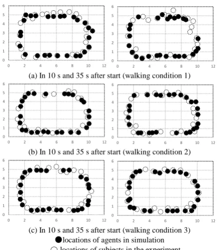
(c) In 10 s and 35 s after start (walking condition 3) ●locations of agents in simulation 〇 locations of subjects in the experiment
Fig. 8. Comparisons of locations of between agent in simulation and subjects in the experiments in three conditions (1st experiment).
The results of the estimation procedure are summarized in Table II, in which the generation number and the minimum value of the evaluation function Eq. (4) were shown. The minimum evaluation values calculated using Eq. (4) are shown in the last column of Table II as the reference value, assuming that the parameters v0, a1, b1, a2, and b2 have the same values for all agents, i.e., the parameters were set to a common value among all agents. Since the evaluation values were smaller than the reference values, the models with the optimized parameters were able to reproduce the observations well.
Fig. 7 shows the change in the value of the evaluation function for each generation for the three walking speeds in the two experiments. It can be seen that the evaluation function values converge. Comparing the parameter estimation time (number of generations) for the flow data of Experiment 1 and Experiment 2, it took a longer time to estimate the parameters of Experiment 2.
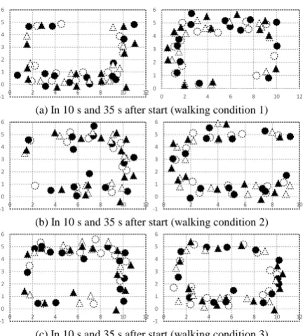
In order to compare the flow in the simulation with experimental flow data, plots of the positions of all subjects and agents in 10s and 35s from the start are shown in Fig. 8 and Fig. 9, respectively. In Fig. 8, the agent position in the simulation is indicated by ●, and the subject position is indicated by ○. Also in Fig. 9, the agent positions moving in a clockwise direction and anti-clockwise direction are indicated by ● and ▲, respectively. The positions of the subjects are indicated by ○ and △. These plots show that the positions of agents in the simulations approximate the experimental data.
This indicates that the global flow characteristics of pedestrians can be represented by the obtained parameters. On the other hand, it is suggested that the dynamic characteristics of human flow may change with time, but it is necessary to continue verifying change in the degree of divergence over time.
-1 0 1 2 3 4 5 6
0 2 4 6 8 10 120
1 2 3 4 5 6
0 2 4 6 8 10 12
(a) In 10 s and 35 s after start (walking condition 1)
-1 0 1 2 3 4 5 6
0 2 4 6 8 10 12
-1 0 1 2 3 4 5 6
0 2 4 6 8 10
(b) In 10 s and 35 s after start (walking condition 2)
-1 0 1 2 3 4 5 6
0 2 4 6 8 10 12
-1 0 1 2 3 4 5 6
0 2 4 6 8 10 12
(c) In 10 s and 35 s after start (walking condition 3) ●clockwise, ▲anti-clockwise location of agent in simulation 〇 clockwise, △anti-clockwise location of subjects in the experiment
Fig. 9. Comparisons of location of agent between experiments and evacuation simulations.in three conditions (1st experiment).
0 0.2 0.4 0.6 0.8 1 1.2 1.4 1.6 1.8 2
1 6 11 16 21 26 31 36 41 46 51 56 61
d if fe re n ce (m ) time(sec)
Exp1.Cond.1 Exp.1 Cond.2 Exp.1 Cond.3
Exp.2 Cond.1 Exp.2 Cond.2 Exp.2 Cond.3
Fig. 10. Change of value of the cost function over time (first experiment).
3) Evaluation of the estimated parameters and discussion
A histogram of the target velocity v0, which is a parameter obtained by the GA method, is shown in Fig. 11. Comparing the parameters estimated for the flow data of the two experiments, the estimated values for v0 in the second experiment distributed in the larger value area than one in the first experiment, reflecting the experimental situation. As the walking speed condition increased, the speed parameter was also distributed in a larger area.
Comparing the results of the second experiment with the first, it is suggested that parameter estimation can be effectively performed by GA based on the I.A., which represents the degree of conformity of the evacuation simulation with the actual data. However, it took longer to minimize the value of the evaluation function in the case of second experiment. This result suggests that the optimization
process was more complicated in the case dealing the flow data of the second experiment.
0 2 4 6 8 10 12
8 10 12 14 16 18 20 22
Fr equenc y parameter V0 0 2 4 6 8 10 12
8 10 12 14 16 18 20 22
Fr
equenc
y
parameter V0
Condition 1 Condition 1
0 2 4 6 8 10 12
8 10 12 14 16 18 20 22
Fr equenc y parameter V0 0 2 4 6 8 10 12
8 10 12 14 16 18 20 22
Fr
equenc
y
parameter V0
Condition 2 Condition 2
0 2 4 6 8 10 12
8 10 12 14 16 18 20 22
Fre que ncy parameter V0 0 2 4 6 8 10 12
8 10 12 14 16 18 20 22
Fr
equenc
y
parameter V0
Condition 3 Condition 3 (a) First experiment (b) Second experiment Fig. 11. Distribution of parameter v0 of the simulators for the data of 1st and
2nd experiments.
From a qualitative evaluation of the parameters obtained, and the extent of the deviation from the measured flow data of the subjects, the divergence after the lapse of time, the parameter estimation method using GA is appropriate. Whilst the model parameters could be estimated, it is necessary to continue verifying the reasons for differences between the simulation and actual measurement data.
The models with the optimized parameters were able to reproduce some of the observations well in some cases, but large divergence between the actual experimental flow and simulated flow also occurred. This result highlights the difficulty of representing crowd behaviors in one single model.
VI. CONCLUSION AND FUTURE WORK
ACKNOWLEDGMENT
This research was funded by JSPS Grant-in-Aid for Scientific Research (C) 16K01295. I express my gratitude here.
REFERENCES
[1] E. Kuligowski, R. Peacock, and B. Hoskins, “A review of building evacuation models,” 2nd Edition, NIST Technical Note 1680, 2010. [2] D. Helbing, I. Frankas, and T. Vicsek, “Simulation dynamical features
of escape panic,” Nature, vol. 407, pp. 487-490, 2000.
[3] J. Holland, “Adaptation in natural and artificial systems,” University of Michigan Press, second edition, 1992.
[4] M. Moussaïd, M. Kapadia, T. Thrash, R. W. Sumner, M. Gross, D. Helbing and C.Hölscher, “Crowd behavior during high-stress evacuations in an immersive virtual environment,” Journal of Royal Society Interface, 2016.
[5] M. Moussaıd, D. Helbing, and G. Theraulaz, “How simple rules determine pedestrian behavior and crowd disasters,” in Proc. National
Academy of Sciences, pp. 6884–6888, 2011.
[6] K. Yasufuku, "Representation of high-density crowd walking using ellipse-based RVO model," AIJ J. Technol. Des, vol. 17, no. 35, pp. 187-190, 2011.
[7] E. Ronchi, E. D. Kuligowski, P. A. Reneke, R. D. Peacock, and D. Nilsson, “The process of verification and validation of building fire evacuation models,” NIST Technical Note 1822, 2013.
[8] A. Johansson, D. Helbing, and P. K. Shukla, “Specification of a microscopic pedestrian model by evolutionary adjustment to video tracking data,” Advances in Complex Systems, vol. 10, pp. 271-288, 2008.
[9] Y. Nonaka, M. Onishi, T. Yamashita, T. Okada, A. Shimada, and R. Taniguchi, “Effective walking velocity modeling for pedestrian simulator,” in Proc. Int. Conf. on Quality Control by Artificial Vision), pp. 131-135, 2013.
Tetsuya Miyoshi was born in Osaka, Japan, in 1963. He received the B.E. and M.E degree in industrial engineering from the Osaka Prefecture University, Japan, in 1987 and 1989, and Ph.D. degrees in industrial engineering from the Osaka Prefecture Universty in 1997. He is currently working as professor in the Department of Management and Information of Hannan University, Osaka, Japan.
He worked as a system engineer in the Osaka prefecture government office at first after getting the M.E., assistant professor in Osaka Prefecture University from 1993 to 1999, associate professor in Hiroshima City University from 1999 to 2002, professor in Toyohashi Sozo University from 2002 to 2015, and onward from 2016.
Prof. Miyoshi is a member of IEEE, Japan Industrial Management and Engineering and SIG on reliability engineering. He is currently interested in the field of reliability and safety of social systems.